Abstract
While a variety of image processing studies have been performed to quantify the potential performance of neural network-based models using high-quality still images, relatively few studies seek to apply those models to a real-time operational context. This paper seeks to extend prior work in neural-network-based mask detection algorithms to a real-time, low-power deployable context that is conducive to immediate installation and use. Particularly relevant in the COVID-19 era with varying rules on mask mandates, this work applies two neural network models to inference of mask detection in both live (mobile) and recorded scenarios. Furthermore, an experimental dataset was collected where individuals were encouraged to use presentation attacks against the algorithm to quantify how perturbations negatively impact model performance. The results from evaluation on the experimental dataset are further investigated to identify the degradation caused by poor lighting and image quality, as well as to test for biases within certain demographics such as gender and ethnicity. In aggregate, this work validates the immediate feasibility of a low-power and low-cost real-time mask recognition system.
1. Introduction
The coronavirus (COVID-19) pandemic continues to have a global impact on our society since its initial spread began in late 2019 [1]. One of the most visually perceptible ways the coronavirus has affected society’s ritual errands and routines is through the widespread use, and in many cases government or commercial mandates, of facial masks intended to slow the spread of the virus by impeding transfer of respiratory droplets via the nose and mouth [2]. Several US states now legally mandate that people wear masks before entering a public space where it is not feasibly practical to socially distance, such as a grocery store. As of early 2021, additional federal mandates [3,4] have been put into place, further extending those requirements.
Independent of the questions associated with mask efficacy or policy, this paper seeks to answer how effectively we can gauge compliance with masking guidelines, as it is uncertain as to how many people actually follow these mandates. Further, the paper seeks to validate the technical capability and implementation feasibility of a sub-$100 Raspberry Pi-scale solution that is suitable for installation at the front door of a store or other congested passageway.
1.1. Motivation
A widespread problem since the inception of the pandemic has been not just the virus itself, but its airborne spread, which is believed to be directly correlated with mask usage [5]. One particular challenge in the present environment is that of mask adherence, which has largely been delegated to ‘gatekeeper’ store employees that can themselves get sick and/or lead to altercations when prompting incoming patrons to don their masks [6,7,8]. Industry is increasingly adopting Internet of Things (IoT) devices that incorporate machine learning for various applications [9]. It is clear that an IoT device presents an ideal solution for helping society adapt to the challenges presented by the pandemic. Therefore, we want to test the feasibility of a more automated machine-based solution that is capable of giving a binary decision as to whether individuals are wearing masks, which may be converted to a visual green/red light that indicates permission to enter; a notional example of this process is depicted in Figure 1. For maximum marketability and deployment versatility, the solution is designed to be capable of processing collected data without requiring cloud or other third-party computing services to ensure that inference decisions are relayed to users reliably and immediately. Our solution lays the initial foundation and identifies the challenges of what we envision will be a fully-automatic ‘mask compliance’ assessment IoT device that can record, analyze, upload, and communicate data to other entities such as epidemiologists, state health departments, human resources personnel, or consumer marketing researchers.
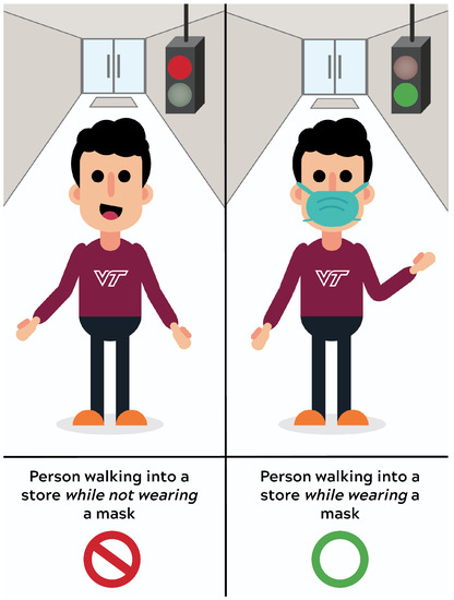
Figure 1.
Conceptual depiction of how automated mask recognition might be used at a storefront, when a camera is placed opposite the hypothetical individual. A visual indicator turns red when an individual is not wearing a mask and green when an individual is wearing a mask, giving immediate feedback about permission to enter.
Lab-based mask recognition performance on pristine images routinely achieves over 99% accuracy using these machine learning techniques [10]. However, in order to be acceptable in a practical context, that performance level must be retained when implemented in a real-world context, using non-pristine images, and in a cost/form factor that is realistic for a store to deploy. Further, knowing that many machine-learning solutions are susceptible to degradation resulting from training dataset mismatch with respect to ethnicity [11], gender [12], image quality [13], lighting conditions [14], and combinations of these parameters with other characteristics [15,16,17], we chose to intentionally bombard the neural net model with different presentation attacks to quantify how quickly performance degrades.
1.2. Research Questions & Goals
A few of the questions that the experimental design and analysis presented in this paper seek to answer include:
- What are the primary features that influence the decision(s) a binary mask recognition classifier will make?
- How many images are necessary for the model to ultimately identify whether an individual is wearing a mask (i.e., select the correct label)?
- How and why do ‘real-world’ scenarios affect performance, versus tests in controlled environments?
- Can a sufficient machine-based performance be achieved and scaled to that of a low-cost real-time platform?
1.3. Prior Work
There are several existing mechanisms for face detection [18,19], which seeks to identify the presence and location of a face, as opposed to face recognition [20], which seeks to find an identity for a face, which is not the focus of this paper. These mechanisms include feature-based object detection, [21], local binary patterns [22,23], and deep learning-based approaches [24,25,26].
Viola-Jones face detection [21] is an object detection algorithm for identifying faces in an image using a Haar feature based cascade of classifiers. Haar features [27] are the difference of pixel intensity sums taken across adjacent rectangular subwindows in detection windows; these features are then used to find regions such as the eyes and nose of a human face based on their intensity levels. Integral images are used to represent the input images, which decreases the computation time of calculating Haar features. A modified Adaboost algorithm is used for classifier construction by selecting and utilizing the most relevant features, based on a threshold set by positive and negative image examples [28,29]. The classifiers are then cascaded, which ensures a low false-positivity rate.
Convolutional neural networks (CNNs) are a type of neural network that can be applied to myriad tasks, such as image classification, audio processing, and object recognition. Face detection and recognition is a natural application for CNN algorithms, which have many different architectures. For example, MobileNetv2 [30] is a model architecture that incorporates inverted residual blocks with linear bottlenecks to decrease network complexity and size. The ResNet [31] (residual neural network) architecture utilizes deep residual learning to decrease deep network complexity and necessary computations, while also increasing performance. ‘Shortcuts’ between layers are used to preserve the inputs from previous layers, which are then added to the outputs of the succeeding layers. Common configurations of ResNet include 18, 34, 50, 101, or 152 convolutional layers; after the initial convolutional layer, one max-pooling layer is used; before the final fully-connected layer, one average-pooling layer is used. MTCNN [25] (multitask cascaded convolutional neural networks) is a framework that uses cascaded CNNs to infer face and landmark locations from images. Three stages of CNNs are used to find and calibrate bounding boxes as well as find coordinates for the nose, left and right mouth corners, and left and right eyes of a human face.
One significant difficulty within facial detection and recognition systems is occlusions, which introduce large variations to typical facial features. A wide variety of facial detection and recognition methods have been formulated and refined for high accuracy in the case of occlusions in the past few decades. In [32], an adversarial face detector is trained to detect and segment occluded faces and areas on the face. Three varieties of facial datasets, including masks, were assembled in [33], including images scraped from the internet and images that were photo-edited to show faces with masks on. A method for facial recognition of masked faces is also introduced, which improves accuracy over traditional architectures for facial recognition by training a multi-granularity model on the aforementioned datasets in combination with existing face datasets. In [34], a masked face dataset is created and locally linear embedding (LLE) CNNs are introduced for detection of masked faces.
Despite these works, a large masked face dataset with sufficient image feature diversity to be similar to real-world images was difficult to find. Dataset augmentation can be used to supplement the amount of feature variation seen by a model during training as well as the overall size of a dataset.
In [35], the quantity and quality of simulated, captured (collected), and augmented training data is analyzed for their impacts on a radio frequency classification task. Simulated datasets are created via random generation based on set characteristic distributions. Dataset augmentation is carried out in two ways: by sampling from existing collected capture data and modifying it to obtain uniform signal characteristic distributions in the resulting dataset, and by random selection from a Gaussian joint kernel density estimate (KDE) on captured data. One key result shows that augmentation using the KDE of the captured data increases test performance compared to data augmentation without taking into account the distributions of known data parameters, but that in both cases augmentation may increase generalization and improve performance, compared to training with solely the original dataset. One caveat is that as the dataset quality decreases and difficulty increases to a certain degree (the exact threshold was not computed by the authors), and the sample quantity remains fixed, model generalization and performance tend to decrease, especially when using augmented data that was collected without consideration of the existing dataset distribution.
Additionally, the quantity of data samples required for 100% and 95% accuracy based on linear trend and logistic fit data is found to be lower for both of the datasets acquired via the previously mentioned augmentation techniques only with less difficult datasets. For example, the KDE-based augmented dataset necessitated approximately 58% and the non-KDE augmented dataset required 167% of the number of samples per class than the original dataset required to obtain 95% accuracy on the least difficult data analyzed in the paper; on the most difficult data, the KDE-based augmented dataset required 180% and the non-KDE augmented dataset required 330% of the number of samples per class than the original dataset required to obtain 95% accuracy. Although more data is needed for high performance, collecting data for the context of the referenced paper is a time-conserving procedure—generation of augmented data significantly decreases the time required to obtain sufficient samples for 95% performance on the order of years.
Essentially, the results relevant to the work presented in the following sections of this paper are that (1) utilizing the statistical properties of the original dataset when assembling an augmented dataset is crucial to ensuring model generalization is improved and (2) the augmented dataset will have an overall lower quality of data than the original dataset and should include a greater number of samples from each class than the original dataset to ensure high performance on more difficult test data.
Independent measures of quality and other properties may cross-check and/or improve the confidence of a neural network’s classification decision. These measures also may improve performance as human-assigned categorical labels are prone to human error and consequently mislabeled data, which has a negative impact on classification performance [36]. BRISQUE (Blind/Referenceless Image Spatial Quality Evaluator) [37] is a spatial image quality assessment (IQA) method that does not use a reference image. The statistical regularity of natural images (i.e., images captured by a camera and not images created on a computer) are altered when distortions are present. Based on this, BRISQUE extracts features from an image based on its MSCN (Mean-Subtracted Contrast-Normalized) coefficient distributions and the pairwise products of the coefficients with neighboring pixels in four directions. For these inputs, the best-fit mean, shape, and variance parameters to an asymmetric or symmetric generalized Gaussian distribution are used in the feature vector, which is then mapped to the final quality score via regression. Furthermore, we believe that BRISQUE is a reasonable method for real-time image quality assessment because it is highly computationally efficient. In the paper, using a 1.8 Ghz computer with 2 GB of RAM, a 512 × 768 image took only 1 s to process. This is much faster than two other IQA algorithms, DIIVINE [38] and BLIINDS-II [39], which took 149 and 70 s, respectively.
1.4. Paper Outline
The organization of this paper is as follows: Section 2 begins with an overview of the experimental framework for testing the feasibility of a real-time mask recognition system. The selection and modification of the dataset used is described in Section 2.1. In Section 2.3, scenarios for characterizing imperfect image capture conditions are described, including how performance is affected by head pose variations and a variety of presentation attacks. Section 3 outlines an experiment where video-recorded participants were encouraged to attempt presentation attacks; although relatively small in dataset size, these results offer insight into how quickly categorical data labeling and unexpected/untrained stimuli degrade overall system performance. Section 4 describes the process of capturing and analyzing real-world video recordings of pedestrians using a laptop and a webcam; both results of these real-time evaluations and extrapolations to expected number and frame rate of images required for a correct inference are presented. Finally, Section 5 offers overall conclusions from our experiment and suggestions supporting near-term implementation of a real-time low-cost platform capable of performing mask recognition on a commercial scale.
2. Experimental Design & Methodology
Implementation of real-time inference for binary classification (i.e., whether or not a person is wearing a mask) on a webcam-equipped PC or a low-cost device could help bolster local health administration statistics and evaluation of the efficacy of current policies. A graphical summary for our experimental model is presented in Figure 2. For further clarity, the process shown in Figure 2 is described as pseudo-code in Algorithm 1.
| Algorithm 1: Mask recognition system functional process for multiple image files. |
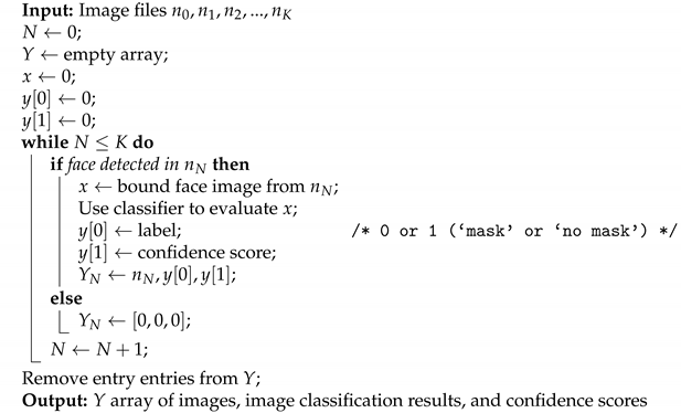 |
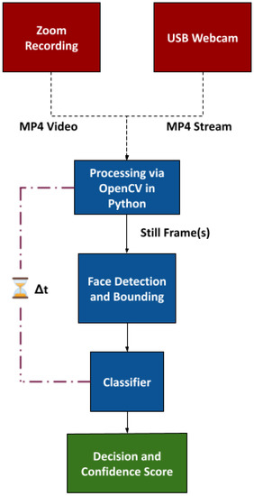
Figure 2.
Preliminary architecture.
To examine this setup further, two neural network models [30,31] were given a binary classification task with experimental images collected from a recorded video experiment in which participating individuals were encouraged to alter their appearance in ways that may be somewhat unexpected, but not entirely uncommon, in real-life implementations. A few examples of edge cases that were shown to impact classification performance while developing the mask recognition system include people wearing masks with animal faces (such as a dog nose), human faces, or other distracting patterns printed on them, and people with beards or mustaches that extend past the mask. These edge case results are not the focus of this work and were not analyzed fully; further information on these categories can be found in Section 3.2. MobileNetV2 and ResNet-18 were selected as the neural network models to use due to their common use in mobile computer vision applications and the availability of pre-trained models. The architecture was implemented in Python using PyTorch [40], an open source machine learning software framework, and OpenCV [41], a computer vision library written in C++ with bindings for Python. Prior to the execution of any experiments involving human subjects, the Virginia Tech IRB (Institutional Review Board) reviewed the protocol used for this research (IRB 20-736) on 24 September 2020. The protocol was approved and was determined to meet the exemption criteria under 45 CFR 46.104(d) category(ies) 2(ii) [42].
2.1. Dataset Selection & Augmentation
One of the largest published datasets of masked faces is the Real-World Masked Face Recognition Dataset (RMFRD) [33], which contains over 2000 photos of individuals wearing masks and 90,000 photos of individuals without masks, across a total of 525 identities. (Although RMFRD is reported to have 5000 images of individuals wearing a mask, less than half of such images could be successfully obtained from the download links provided in the publication.) RMFRD, the Simulated Masked Face Recognition Dataset (SMFRD) (comprised of images of masks digitally imposed onto faces), and the Masked Face Detection Dataset (MFDD) (similar to RMFRD) are three separate datasets assembled in the same paper under the parenting Real-World Masked Face Dataset (RMFD).
Based on the distribution discrepancy across the ‘mask’ and ‘no mask’ classes, the dataset is highly biased towards the ‘no mask’ label. However, this does not seem to have significantly negatively affected model performance towards ‘mask’-labeled images (at least in controlled environments), as shown in Section 3. In this paper, (in contrast to the process from [35], which is described in Section 1.3), augmentation refers to supplementing the original RMFRD dataset with additional images of people wearing and not wearing a mask. These images were captured from the internet, specifically Instagram (it is worth noting that the set of images from Instagram may be biased towards demographics that tend to use Instagram more frequently than other demographics).
RMFRD consists of typically average-quality images (as described further in this section) with closely cropped faces and homogeneous demographic diversity. To mitigate this, which may cause poor performance in real-world implementations, several hundred publicly-accessible photos were scraped from Instagram using the hashtags #maskon and #maskup. Approximately 2800 images were gathered. MTCNN [25] was used to quickly determine which images contained faces, resulting in 993 images. These images were then manually labeled into two categories, based upon whether or not an individual was correctly wearing a mask. In total, 711 images of individuals without masks and 282 images of individuals with masks were gathered. The unbalanced categories are due to a disparity in image availability. The resulting split used for training is shown in Table 1. Table 2 displays the accuracy for training, validation, and test phases of two CNN architectures on the original RMFRD dataset and on the augmented RMFRD dataset.

Table 1.
Dataset image quantities for classification into ‘mask’ or ‘no mask’ labeled images.
Table 2.
Performance results of MobileNetv2 and ResNet18 on the RMFRD dataset and on the augmented RMFRD dataset.
Two models, MobileNetv2 [30] and ResNet18 [31], were evaluated on the RMFRD training set. Both models were pre-trained on ImageNet. Transfer learning was then utilized to retrain the last layer for classification on masked and unmasked faces. The performance is shown in Table 2. The performance of the original MobileNetv2 model and the augmented MobileNetv2 model on solely the Instagram test set was only 83.28% and 83.59%, respectively. This concept is also displayed on a minute level in Table 2, where the augmented models have a slightly diminished performance compared to the original models. Similarly to the age-old ‘jack-of-all-trades, master of none’ adage, generalization of training data makes network models more broadly applicable to new data, but reduces overall performance due to broadened learned behavior(s). This degradation in observed performance also suggests that there is room from improvement in baseline performance simply by improving the robustness of the dataset(s) during training. As described in Section 1.3 and shown in [35], despite the reduced overall performance, this generalization may also result in better performance on previously unseen data, so no attempts were made to further augment the dataset to prevent over-training.
2.2. Commentary on Dataset Bias and Classifier Evaluation
It should be noted that in Table 2 and Table 3, accuracy is utilized as an evaluation metric for classifier performance, although this is not useful compared to other performance metrics such as F1-scores for datasets with a disproportionate number of samples between classes. Within the augmented dataset (Table 1), ‘no mask’ images account for 33 times the number of ‘mask’ images (13,621 and 416 images, respectively). For future work and reference, more well-suited evaluation metrics for this datasets include receiver operating characteristics (ROC), area under ROC (AUC), and precision-recall (PR) curves [43].
Table 3.
Performance results of original and augmented MobileNetv2 and ResNet18 models on total dataset from recorded video.
Moreover, the 1:33 ‘mask’:‘no mask’ ratio indicates a large dataset bias. Although we attempted to mitigate network bias by independently verifying classifier responses in cases of both ‘mask’ and ‘no-mask’ samples, data collection from Instagram and real-world video recordings did not afford control over which class participants would fall under; a large reduction in performance when considering performance for ‘no mask’ images versus ‘mask’ images was to be expected (and did occur) in field test scenarios such as live recordings. Therefore, independent metrics related to image quality were also evaluated (see Appendix A).
2.3. Realistic Image Capture
The variety of ways in which everyday individuals walk, dress themselves, and interact with each other necessitates characterizing a system meant for real-world implementation in ways that help encompass the environmental factors a neural network might encounter when tasked to make decisions as well as the hardware on which it is deployed. In order to determine the realistic performance of the mask recognition system during real-time operations, algorithm performance was tested via still images derived from video recordings at different frames-per second (FPS) rates. Such comparisons help scope the cost and quality of the deployment system. This is described more in-depth in Section 4.2.
2.3.1. Angle Variations & Performance
To estimate the performance of the CNNs in situations where faces appeared off axis, a controlled experiment was devised to evaluate images of an individual (a) wearing a mask and (b) not wearing a mask while moving their head pose across different azimuth and elevation angles. The img2pose PyTorch package for facial detection and alignment was used to obtain the angles [44]. Figure 3 and Figure 4 display the side-to-side and up-down angles of the head pose, plotted by performance from the frame of reference of the camera. A coordinate of 0 azimuth and 0 elevation corresponds to an individual facing the camera along its boresight without moving their head to the left, right, up, or down. A coordinate of negative elevation means the individual was looking upwards. A coordinate of negative azimuth means the individual was looking to their left. Each point in Figure 3 and Figure 4 represents a recorded image in terms of head pose orientation and the output probability score of the correct label being assigned—i.e., ‘mask’ or ‘no mask’. The performance of the augmented MobileNetv2 model was 78.57% and 84.50% for the ‘no mask’ and ‘mask’ image sets consisting of 42 and 71 images, respectively.
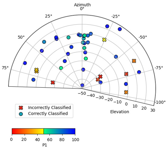
Figure 3.
Scatter plot of azimuth and elevation head angle and performance for the individual not wearing a mask.
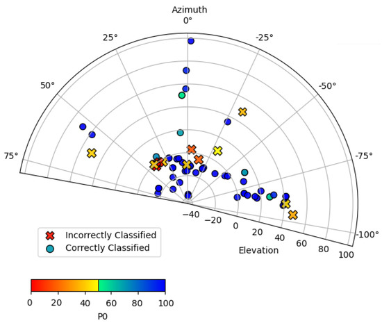
Figure 4.
Scatter plot of azimuth and elevation head angle and performance for the individual wearing a mask.
Similarly to the results in Section 3, the ‘no mask’ performance is worse than that of the ‘mask’ performance. However, due to the wider variation of angles in the ‘no mask’ test, as well as the smaller number of images, it is inconclusive to say that ‘no mask’ performance is always worse than ‘mask’ performance. The results of both trials show that, in general, classification performance decreases at greater tilts of the individual’s head, yet the performance is reasonably stable over the ranges that a person walking towards the entrance of a building would normally exhibit. We infer, based on Figure 3 and Figure 4 that for an individual wearing a mask, that the model is particularly sensitive to changes in azimuth (side-to-side) head pose variations, yet reasonably robust to elevation.
2.3.2. Presentation Attacks
A major consideration in the design of the experiment covered in Section 3 is the inclusion of presentation attacks [45,46] that would intentionally try to degrade the performance of the neural networks used. A few examples of these attacks include:
- Masks of different shapes, sizes, colors, or textures between recordings (e.g., neck scarves, respirators);
- Facial or hair styles that can be easily put on or taken off, such as eye makeup, glasses, ponytails, etc.;
- Hats, scarves, or other partial head coverings worn at different angles and/or worn to cover the face in different ways (such as occluding eyebrows);
- Wearing Halloween masks, wigs, and/or costumes;
- Tilting of webcam off-axis;
- Using facial augmentation filters such as those from Facebook Messenger, Tik Tok, Snapchat, or other apps;
- Having pictures of other people in the foreground or background, such as with posters;
- Placing pets wearing masks or variations (e.g., dog wearing hat) in front of webcam;
- Holding a dog or cat while you are in front of the webcam;
- Using a variety of Zoom backgrounds;
- Positioning the webcam so that the lighting varies, such as facing the sun or in a dark room;
- Changing facial expressions in odd ways (e.g., intentionally closing or crossing eyes).
An important note of these presentation attack scenarios is that participants maintained their chosen state of ‘mask’ or ‘no mask’ during that single instance of time on camera, while changing variables between times on camera; as such, the mask recognition algorithm was not presented with dynamic scenarios of an individual donning or doffing their mask.
3. Recorded Video
Two experimental sessions were recorded over Zoom, a software application for remote video conferencing [47]. This enabled data collection from participants without needing to interact with them at a close distance. Furthermore, this remote setup allowed for recordings that spanned more environmental surroundings, behaviors, facial expressions, hair styles, mask designs, etc., than could be collected via a public data collection system (such as on a street), since each participant had complete access to their personal wardrobe and effects.
Following confirmation of Institutional Review Board (IRB) disclaimers and that all participants were in a location where they may have safely chosen not to wear a mask, individuals were prompted to randomly appear on screen via an audio cue so that the Zoom client recorded the individual. Individuals were instructed to correctly or incorrectly wear masks, to not wear masks, or to follow some randomly chosen variation of mask-wearing listed in Section 2. The variations performed by the individual were recorded for approximately 5–15 s each.
Following the sessions, the recorded MP4 files were imported and processed using OpenCV [41] to convert the videos into still images at approximately 1FPS. The first session was recorded for 45 min and 50 s, resulting in a total of 2749 frames. The second session was recorded for 40 min, 20 s, for a total of 2419 frames. In total, 5168 still frames from 86 min, 10 s of recorded video were obtained from the experimental sessions, which involved 13 individuals. The authors were present in both sessions and are therefore a larger percentage of the final dataset.
The still frames were manually labeled for the presence of a mask, no mask, or an incorrectly worn mask. This process was aided by the development of a Jupyter Notebook [48] that allowed a human to manually label the frames and check for the presence of certain attributes, such as glasses. An example of this labeling acceleration tool is displayed in Figure 5. Although the Jupyter Notebook tool was a significant aid for this work, a strong suggestion for future attempts in labeling a large number of images in a limited time frame is to utilize or improve upon existing methods for ensuring image labels are reliable and accurate, such as in [49].
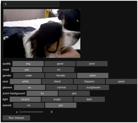
Figure 5.
Example of custom Jupyter Notebook labeling process.
3.1. Results of Recording Analysis
Due to the nature of the training dataset images, the performance of both the MobileNetv2 and ResNet18 model was negatively impacted by the initial images saved from the recordings, which were zoomed out from a face and included the background details, such as a desk or house plant. To mitigate this, MTCNN [25] was used to first identify faces in the images with a 10 pixel bounding box margin. The images were then cropped to only include the face and resized to 240 × 240 pixel. One significant problem presented by this method was that in the case of images containing facial occlusions, such as a mask or pet cat, MTCNN did not bound a face; this issue occurred in approximately 1000 images. These images were separated from the correctly bound faces and manually cropped. A total of 162 images that did not contain faces were removed from the original dataset, resulting in a total of 5007 images.
The resulting performance of the original models and of the augmented models on the edited dataset is given in Table 3. The augmented MobileNetv2 model achieved the highest accuracy at 72.91%, closely followed by the original MobileNetv2 model with an accuracy of 72.59% and the augmented ResNet18 model with an accuracy of 71.73%. The original ResNet18 model had the poorest performance at 69.1%. While these figures are substantially lower than that of the >99% accuracies obtained with pristine images, they are representative of (1) the incorporation of real-world time-varying environments around the faces of interest, (2) the use of partially tuned open-source image pre-processing tools to convert that real-world scenario into still images sized for the neural net, and (3) intentional manipulations of the environments and/or anticipated characteristics affecting learned behaviors of the neural net algorithm in an attempt to fool classification. Further, these accuracies are representative of individual images taken at 1FPS, leaving the potential for further decision accuracy improvement by combining results of multiple images at a higher frame rate as discussed in Section 4.2.
The relatively poor results in Table 3, Table 4, Table 5 and Table 6 were anticipated due to the odd nature of the recorded video sessions. Relatively few ‘normal’ images of individuals wearing or not wearing masks were taken, as compared to a typical setting encountered at an office or supermarket. To further refine the above analytical results, the images were thinned to exclude irrelevant images and images of extremely poor quality, as described in the following section.
Table 4.
Results of recorded Zoom sessions across 8 categories for describing attributes of participating individuals’ appearances.
Table 5.
Performance results of MobileNetv2 model on Zoom dataset. ‘Y’ and ‘N’ stand for ‘Yes’ and ‘No’, respectively, and are used to indicate the number or percentage of images that were correctly classified (‘Y’) or incorrectly classified (‘N’). ‘Other *’ images are defined as those that were qualitatively judged to be anomalous compared to the rest of the dataset.
Table 6.
Performance results of ResNet18 model on Zoom dataset. ‘Y’ and ‘N’ stand for ‘Yes’ and ‘No’, respectively, and are used to indicate the number or percentage of images that were correctly classified (‘Y’) or incorrectly classified (‘N’). ‘Other *’ images are defined as those that were qualitatively judged to be anomalous compared to the rest of the dataset.
3.2. Notes on Qualitative Assessment
An ‘other’ label category was included in the manual labeling of the recorded video frames due to the number of oddities making certain images unable to be classified. This definition was a qualitative assessment of whether the image represented a scenario where a human user would make a correct decision and/or represented too great of a diversion from a normal face (and therefore an aberration in behavior that itself would stick out) to expect the algorithm to make a correct decision. An example of such an ‘other’ image is shown in Figure 6. The 1100 ‘other’ images were set aside for portions of the performance analysis. For the augmented MobileNetv2 model, removing ‘other’ images increased mask classification performance from 63.72% to 77.21%, as shown in Table 5, confirming the expectation the performance degrades when presented with untrained stimuli. An important note, however, is that the failures appeared to be more random than systematic, suggesting the opportunity for a higher level decision agent to arbitrate streams of decisions.
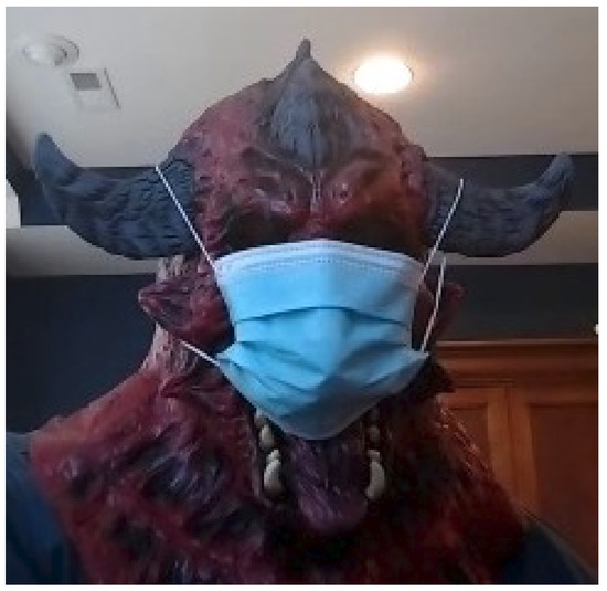
Figure 6.
Example of ‘other’-category image. The individual is definitely wearing a mask, but are they wearing it properly, and what would their gender and race be labeled as?
Furthermore, image quality was assessed qualitatively during the manual labeling process, leading to stratified classification accuracies as shown in Figure 7. The ‘quality’ parameter proved to be of significant importance when evaluating the performance results of the experiments in this paper. As shown in Appendix A, Figure A2, Figure A3 and Figure A4, excluding images marked as ‘poor’ and ‘average’ quality increases overall performance and will assist with requirements definition of the camera and/or image capture setup in a deployed solution.
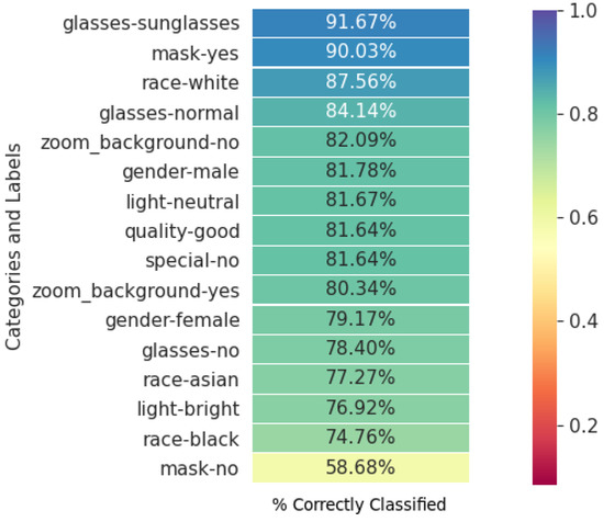
Figure 7.
Heatmap of classification performance with augmented MobileNetv2 model. Ranked order map of performance results on data filtered to remove ‘other’ category and ‘poor’ or ‘average’ quality images.
Quantitatively describing the quality of an image is a more complex task than it initially seemed; in fact, the overall existence and nature of a ‘quality measure’ has come into question. These questions, partially asked and answered in [50], have straightforward solutions; a good quality metric for facial images separates images that improve recognition performance from those that impair recognition performance. The ‘meaning of existence of the quality metric’ remains vague in the scope of this paper, given that we are evaluating mask presence rather than generic facial characteristics, but is a subject of investigation for future work. A rank-order comparison of the underlying parameter labels, and their corresponding differences when only qualitatively-assessed ‘high’-quality images are retained, are shown in Figure 8 and Figure 9.
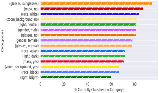
Figure 8.
‘Good’ (qualitative) quality image test performance with augmented MobileNetv2 model across categories. Plot of categorical labels and classification performance with qualitative quality evaluation.
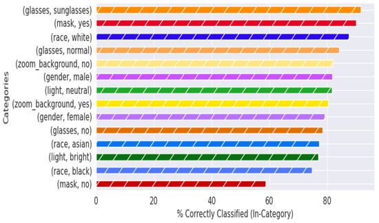
Figure 9.
‘Good’ (BRISQUE) quality image test performance with augmented MobileNetv2 model. Plot of categorical labels and classification performance with BRISQUE quality evaluation.
The BRISQUE method introduced in [37] was selected to quantitatively evaluate the Zoom dataset, because it is a ‘no-reference’ IQA algorithm (i.e., it does not require an image of good quality to assess a new image) and because of its speed compared to other no-reference IQA algorithms, thus making it feasible for real-time implementation of the mask recognition system. The BRISQUE quality measure was separated into three categories, similar to the original subjective quality measure, based on thresholds one standard deviation below and above the mean score for the training dataset. Using a quantitative measure both decreased the chance of a mislabeled image being categorized incorrectly and decreased any human bias present in the quality category. On both the original RMFRD and RMFRD-Instagram augmented test sets, a roughly 5:90:5 {‘poor’:‘average’:‘good’} breakdown was observed in terms of BRISQUE quality, using the same threshold levels to assign the categorical labels as was used on the Zoom dataset. The Zoom dataset had a 15.3% ‘poor’, 71.4% ‘average’, and 13.2% ‘good’ label split.
Figure 8 and Figure 9 display the classification performance across each category (i.e., about 80% of all of the images with individuals labeled as ‘male’ were classified correctly). The primary difference (that will be explained further in the paper) to note between these two figures is within the ‘mask’ and ‘no mask’ labels, which, respectively, swap places as the second-highest performing category between Figure 8 and Figure 9. The metadata labels were chosen to include standard demographic data such as gender and race, as well as common variations observed in individual appearances during the experimental recording sessions. The poor performance within the ‘race’ category for individuals categorized as ‘asian’ or ‘black’ can be attributed to the lack of data across multiple participants for those categories; the majority of participating individuals were categorized as ‘white’. The small sample size also contributes to extreme performance for female participants, individuals wearing sunglasses, and for dark illumination conditions. This is further visualized in Appendix A.
Figure 10, Figure 11, Figure 12 and Figure 13 are stacked probability histograms that complement the figures of Appendix A by illustrating the probability distributions on the vertical axis across each category and its labels across the classification confidence scores on the horizontal axis. The kernel density estimate (KDE) is also displayed as a visual aid for comparisons. In Figure 12 and Figure 13, the small sample size for high quality images is apparent for images of black individuals, individuals wearing sunglasses, and in dim and bright illumination settings.
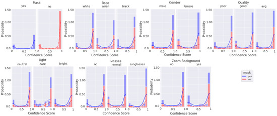
Figure 10.
Histogram of categorical labels vs. confidence scores for all image qualities, as qualitatively evaluated, using the augmented MobileNetv2 model. For each category and its labels, ‘mask’ and ‘no mask’ data bins are stacked. The solid and dashed lines represent the KDE for ‘mask’ and ‘no mask’ image scores, respectively.
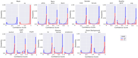
Figure 11.
Histogram of categorical labels vs. confidence scores for all image qualities, as evaluated via BRISQUE, using the augmented MobileNetv2 model. For each category and its labels, ‘mask’ and ‘no mask’ data bins are stacked. The solid and dashed lines represent the KDE for ‘mask’ and ‘no mask’ image scores, respectively.
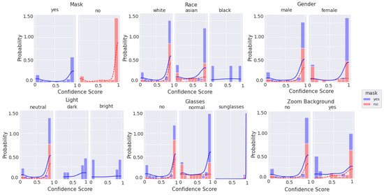
Figure 12.
Histogram of categorical labels vs. confidence scores for only good quality images, as qualitatively evaluated, using the augmented MobileNetv2 model. For each category and its labels, ‘mask’ and ‘no mask’ data bins are stacked. The solid and dashed lines represent the KDE for ‘mask’ and ‘no mask’ image scores, respectively.
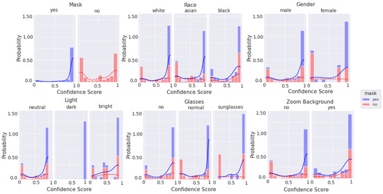
Figure 13.
Histogram of categorical labels vs. confidence scores for only good quality images, as evaluated via BRISQUE using the augmented MobileNetv2 model. For each category and its labels, ‘mask’ and ‘no mask’ data bins are stacked. The solid and dashed lines represent the KDE for ‘mask’ and ‘no mask’ image scores, respectively.
3.3. Uncategorized Data
Images from the Zoom dataset labeled as ‘other’ contain an assortment of different conditions that may confound results from the dataset as a whole. Many of these images were difficult if not impossible for a human to classify as having an individual wearing a mask or not. For example, Figure 5 is an image of a dog wearing a mask. Other examples of images in this category contain people wearing Halloween masks, substantial occlusions caused by objects held in front of the face, etc. A richer dataset, generated in a more controlled context, would be necessary to quantitatively measure the degradations of each of these factors.
4. Live Recording
To extend our experiment one step closer towards real-world deployment, a camera was setup to capture recordings of individuals walking in public with masks on. The recordings were transferred via USB cable to a laptop computer, where they were then evaluated in near-real-time as the video was being captured and as still frames extracted from the video data. The emphasis of this trial was to evaluate the system as implemented in real-world scenarios with variations in illumination, demographics, and angles.
A Logitech C922 Pro Stream web camera [51] with 720P recording at 10FPS, 1280 × 720 resolution was used to test near real-time performance. A JupyterLab notebook was used to capture input from the webcam. Haar face detection was used to identify and bound faces in a frame. For testing purposes, frames containing detected faces were first saved to a PC, then input to the CNN. The label confidence values were averaged over 15 frames to improve performance accuracy. Widgets [52] were used to display the confidence of the label predictions as they were calculated. The total cost of this experiment, not including the laptop computer used for running the model, was approximately $150USD.
Recordings were captured in Blacksburg, Virginia on the Virginia Tech campus in public locations where there are frequently many people walking, such as near libraries, dining halls, and parking garages. Figure 14 illustrates a prime example of a recording location. All of the video recordings were taken during the day, but weather variations contributed to data capture of individuals in sunny (bright) and cloudy (normal to dark) illumination conditions. The time recorded per session varied between 10 and 25 min. In two attempts to record data, areas where crowds were expected—a typically populated open field and a scenic pond with ducks on the Virginia Tech campus—human encounters were few and far between, so the session was cut short. The most fruitful recording was captured at the Blacksburg Farmer’s Market, located adjacent to the university campus. This session consisted of 22:01 min of video capture including camera setup, readjustment of the lens, and time in which no people walked closely past the lens. In total, images across over twenty individuals were evaluated; individuals with an insufficient number of suitable images, at too far a distance, or ones not facing the camera were not included.
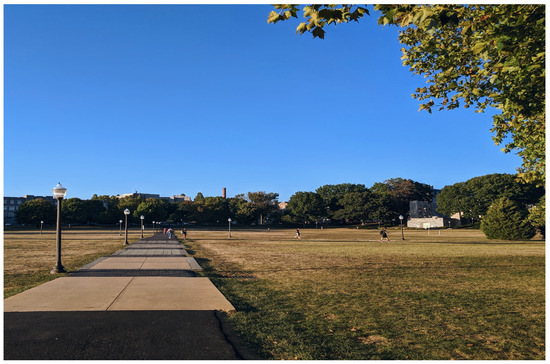
Figure 14.
The Virginia Tech drillfield is a typically popular spot for students to gather; this image serves as an example of a potentially ideal spot to record live data for analysis.
4.1. Results of Live Recordings
The live experimental video captures proved to be more challenging than anticipated from both a practical and technical perspective. The session at the Blacksburg Farmer’s Market was affected by numerous factors: a poor choice of camera setup in which too many people and too many faces would be recorded at once, from too far away (approximately 20ft). The weather also made some faces difficult to detect even when people walked directly towards the camera, due to sun glare and reflections. From a subset containing 173 images that were manually labeled, after face detection and bounding, 18%, 68%, and 13% of the images were, respectively, categorized as ‘poor’, ‘average’, and ‘good’ via BRISQUE quality evaluation. When input to the model, overall accuracy was only 67.05%; however, when filtered to contain only ‘good’ quality images, 90.47% accuracy was achieved.
Initially, the live recording system was programmed and tested using a webcam placed directly in front of a test subject. From a detected face, 15 consecutive frames were taken. In a controlled environment, each frame capture and inference on average took an average of 120ms. Inference post-frame capture and processing took on average 60ms. The total time for a decision was on average 2 s. In contrast to this design, individuals in the live recording testing frequently did not face the camera, even when it was placed in an area that would seemingly encourage facing forward, such as a library entrance. This was especially problematic for Haar facial detection; if a face was not detected, it could not be bounded and input to the model, essentially adding more total time per individual to make a decision. Furthermore, individuals often walked in groups of two or more people. This made it difficult to obtain consistent performance results, as the system would often recognize different faces every few frames. However, the data flow could easily be reworked to display confidence results for each face recognized as opposed to a display of a single result and visualization plot for an individual.
The images gathered from these sessions consisted of typically young to middle-aged Caucasian adults. Additionally, no individual was seen without a mask on. One way to remedy this would be to record data in a setting where less people wear masks, but in a safe way for those around them: e.g., on a running trail or a dog park, where it has been observed by the authors that people adhere to social distancing principles while not wearing masks. Table 7 contains the categorical result counts. In contrast to Table 4, which contains the results counted by number of occurrences over all of the image frames, Table 7 contains the unique individual counts over the entire video recording (e.g., a Caucasian woman wearing a mask and occurring in multiple frames was only tallied once for Table 7).
Table 7.
Results of live recordings across 5 categories for describing attributes of individuals’ appearances.
Further implementations of this setup would be improved by incorporating image pre-processing to correct for exposure and contrast before attempting to detect a face. An additional observation was that many people avoided the camera, which was intentionally placed in a conspicuous location. Additional experiments may be benefited by camouflaging the camera and tripod, or placing LED lights or other attention-grabbing mechanisms around the camera so that individuals are more likely to willingly look approximately into the boresight of the camera.
4.2. FPS Analysis
In order to determine the optimal performance of the system for a given FPS, a two-minute recording was selected and processed at 1FPS, 2FPS, 3FPS, 10FPS, and 30FPS. This process was used to find the effective decision accuracy of the system; i.e., how many ‘good’ decisions are needed based on the number of images to be evaluated in order to make a correct inference, and how long (how many frames) are necessary? Through bifurcation of a set of images to be evaluated based on quality, three separate approaches to this analysis are explored:
- Discard: Toss the ‘bad’ images based on BRISQUE quality assessment and classify k images based on the remaining images.
- Consensus: Implement a voting system so that in a set of images of quantity k, classification decisions made on higher quality images are weighed more heavily than those made on poor quality images.
- Discard, then find consensus: Combine the ‘discard’ and ‘consensus’ mechanisms by first throwing away poor quality images, and making the final classification decision by weighing the individual inference outputs from the remaining images according to their quality score.
The Discard method is based on the BRISQUE quality score of the images. Images with a score above the second quartile of the quality scores from the image set were not considered for classification decisions. The mean confidence output of the remaining images was calculated and used as the final output classification. The Consensus method uses all images, but weighs each decision based on the quality score of the image and the confidence score of the inference decision. Scores below the first quartile are given a 1.25x ‘vote’, scores above the first quartile, but below the second quartile are given a 1x vote, and so on and so forth for the remaining quartiles. The Discard + Consensus method simply consists of the aforementioned methods combined sequentially.
Table 8 displays the performance results for video of an individual wearing a mask sampled at 1, 2, 3, 15, and 30FPS. The set of {N = 3, 5, or 10} images were selected in consecutive order as to simulate a real-life scenario. Overall, first discarding images of poor quality, then weighting votes for classification generally improves the probability P of a correct classification score. However, it is important to note that these results are from a single video; additional images and testing of these methods is an effort to be undertaken in future work. Furthermore, the analysis of binomial reduction of multinomial classification decisions across multiple real-time images is being separately prepared for publication.
Table 8.
Results from video sampled at varying FPS rates. N is the number of images used. P is the overall probability of correct classification based on N images. M1, M2, and M3 refer to the ‘Discard’, ‘Consensus’, and ‘Discard + Consensus’ methods described in Section 4.2 for image selection.
5. Conclusions & Future Work
Summarily, the main contributions of this work are twofold:
- A unique experimental dataset in which participants of varying demographics were encouraged to try presentation attacks was recorded, manually labeled, and evaluated. The primary finding from the analysis was that the model performs reasonably well on individuals wearing and not wearing a mask provided that the image quality is sound. Furthermore, quantitative image quality was found to impact the distributions of the results as compared to qualitative image quality, which is subject to the typical problems associated with human behavior (i.e., bias and errors.)
- The characterization of the feasibility of real-world implementation of a mask recognition system, including consideration of hardware resources and time in terms of frames captured. This analysis also took into account how real-world conditions such as lighting variations due to weather and head angle changes may impact performance of the system, and how to mitigate this impact by recording for the necessary number of frames necessary for a high-confidence classification.
Our development of a practical mask recognition system architecture, dataset assembly and analysis, and investigation into the occurrence and mitigation of the problems incurred during image and video capture in imperfect, uncontrolled ‘real-life’ scenarios serves as a useful stepping stone for other IoT research seeking to deploy smart devices in realistic settings in industry and consumer markets. Additionally, our solution was created to be easily and inexpensively implementable on devices which are even less capable than a consumer laptop, such as an Arduino or Raspberry Pi; these hardware devices are accessible, simple, and can be interfaced with existing IoT devices in a given use case scenario (such as a ‘smart’ supermarket).
One consideration for any candidate hardware system is ensuring that the processor adjusts to the frame rate of video recordings in order to optimize performance in regards to the capabilities of both the camera and the computing system. Additionally, re-training the model for each location could be accomplished with relative ease: training data could be gathered by having a store associate manually label captured images of customers walking into the establishment, via a clicker button or Jupyter Notebook (similarly to the process used for manual labeling in this paper); this new data could then be utilized for re-training a model to be deployed. This would result in a uniquely trained model for each location that the mask recognition system would be used in. Although the performance impact caused by differences in illumination, camera position, and background objects in a new setting versus the typical training data setting is unclear, the aforementioned re-training process would help remedy any negative affects due to a change in location.
There remains a fundamental question as to whether or not a neural network is ‘overkill’ for this application. This could be revealed by testing other methods for classification. For example, a Haar cascade classifier could be trained to bound the eyes, nose, and mouth of a human face; the absence of a nose or mouth could be used to classify whether or not a mask is present without the use of a neural net. The results found in the experimental sessions show that performance is primarily affected by image quality and head pose. Image quality is a broad area of research; this paper used the BRISQUE algorithm, which does not utilize distortion-based metrics (such as blur). A wider exploration of evaluation methods may reveal different impacts on classification performance than shown in this paper. One significant issue found across the architecture in Figure 2 was the importance of face bounding prior to inference. Investigation into faster, smaller, and more accurate methods than Haar cascade classifiers and MTCNN for this would be helpful for real-world implementations.
Computer vision algorithms may seem excessively computationally intensive for IoT devices. However, they have been implemented on devices such as the Raspberry Pi for many machine learning-based image classification and recognition applications [53,54,55]. Moreover, some of these implementations utilized software packages that were also used for the mask recognition system, such as OpenCV [56]. Based on the aforementioned information, in addition to the fact that the algorithms and software used in our solution are well-recognized by the computer vision and machine learning communities, it can be stated that our mask recognition system is feasible to implement on low-cost, low-power edge computing devices such as the Raspberry Pi.
Additionally, no specific distribution of image properties (such as file format (e.g., PNG, JPG), pixelation, and intensity), nor demographic characteristics (such as race and gender) were targeted when the images were collected other than whether or not the subject of the image is wearing a mask. As detailed in [35], it is straightforward to speculate that analyzing the parameter distributions of the RMFRD training set images and then augmenting the training dataset with additional images either collected from other sources or modified after collection such that the resulting dataset has a more uniform range of parameter distributions (as compared to the original dataset) may enhance the model’s ability to generalize and improve test and implementation performance compared to the results in this paper. Further, we believe that model performance will also improve if the training dataset is independently augmented with images in the specific environment of interest (e.g., each independent installation of the mask recognition device is updated during installation), though that expectation was not sufficiently tested.
Ultimately, the fundamental goal of this work was to prove the feasibility of low-cost deployment of a mask recognition system with acceptably high confidence outputs. In lieu of Jupyter Widgets, a red/green traffic-light style indicator could easily be integrated with the setup to provide feedback. Furthermore, implementation on a low-cost, low-power development platform with IoT capabilities, such as a Raspberry Pi or Arduino, could be easily adapted to deploy the mask recognition algorithm in real-world scenarios, where it could send data to other devices and parties, as well as be modified for new image assessment tasks. For example, some regions have begun to implement a program that issues QR codes to vaccinated individuals so that proof of COVID vaccination can be shown before entry to a public place is granted [57,58]. It can be stated that modification to the presented mask recognition system to give it the capability to capture and process a QR code input to the system by an individual would be trivial to implement, as minimal-to-no physical changes would be necessary—a camera and computing hardware device are already present, and cloud computing resources could be utilized if needed. Although the technical specifications of QR codes and their security practices are outside of the scope of this paper, the validity of the QR codes showing vaccination status has already been a consideration for existing health software utilities. For example, SMART Health Cards include vaccination history within a QR code and are verified by a mobile application that flags unauthorized modifications to the card and checks that the code issuer is part of a trusted network of health providers [59]. A similar approach could be applied to the mask recognition system.
In conclusion, this is an easily-marketable experimental setup that could be produced inexpensively. The authors encourage those with an interest to replicate and improve the work in this paper based on the suggestions given above and lessons learned about implementation.
Author Contributions
Conceptualization, R.M.B. and A.J.M.; methodology, R.M.B. and A.J.M.; software, R.M.B.; writing—original draft preparation, R.M.B.; writing—review and editing, A.J.M.; visualization, R.M.B. and A.J.M.; supervision, A.J.M. All authors have read and agreed to the published version of the manuscript.
Funding
This research received no external funding.
Institutional Review Board Statement
The study was conducted according to the guidelines of the Declaration of Helsinki, and approved by the Institutional Review Board of Virginia Tech (protocol code 20-736, 24 September 2020).
Informed Consent Statement
Informed consent was obtained from all subjects involved in the study.
Conflicts of Interest
The authors declare no conflict of interest.
Appendix A. Supplementary Material Regarding Qualitative vs. Quantitative Image Assessment
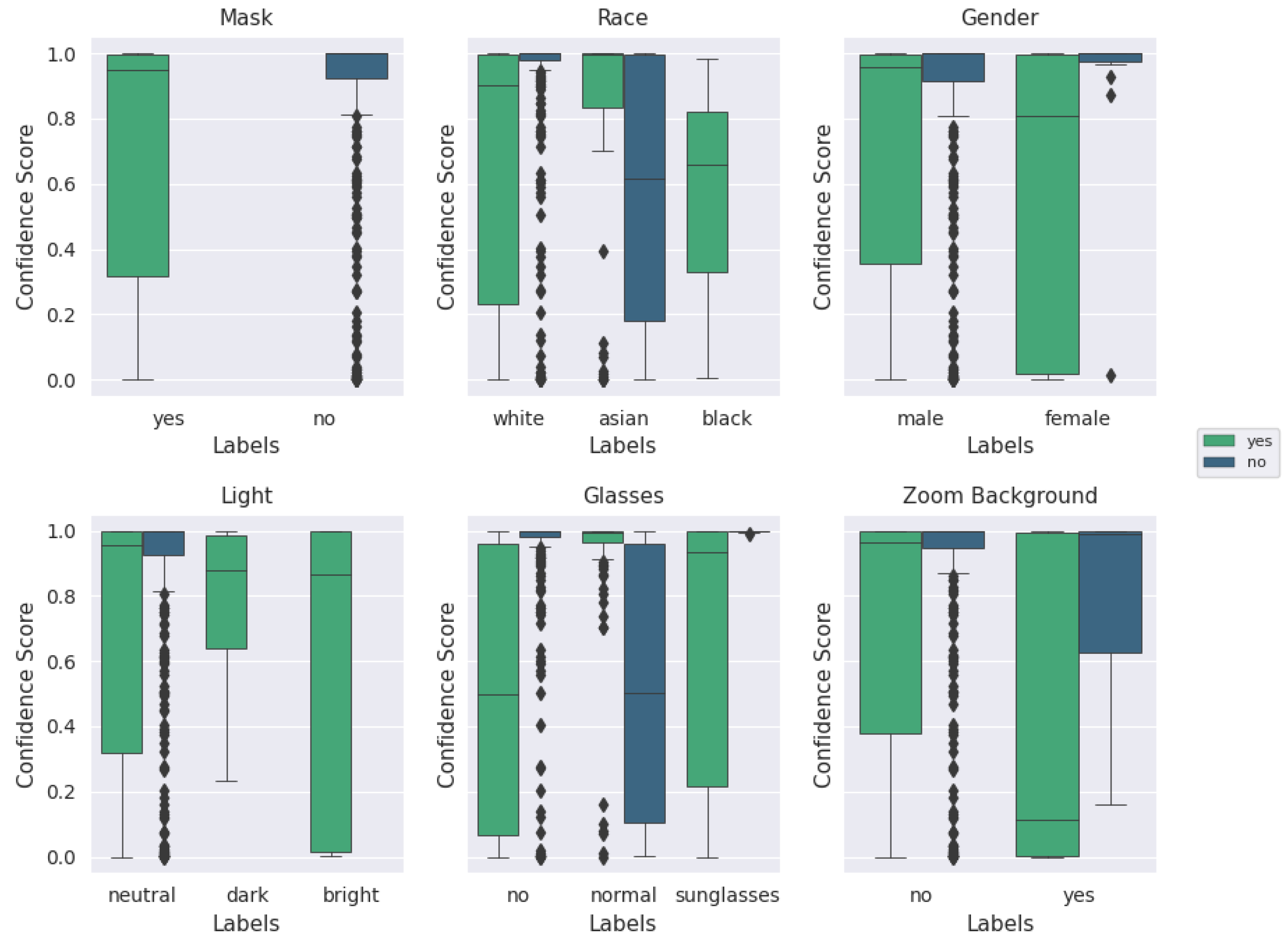
Box plots are a useful way to illustrate basic statistics in a set of data, thus simplifying the identification of relationships and distributions that may lie within the data [60]. The upper and lower extrema are represented by the top and bottom lines, respectively; similarly, the upper and lower quartiles are represented by the top and bottom of the box. The median of the data is represented by the center line. For this application, box plots help visualize how each category and label are related to the confidence score output (described below) by the model during classification. Figure A1–Figure A4 consist of box plots displaying the categorical label distributions for ‘mask’ and ‘no mask’ images. On the vertical axes, confidence scale refers to the outputs from the model for the correct classification label: during evaluation, a softmax function is used to scale the two model outputs between 0 and 1 so that the sum is 1. corresponds to the ‘mask’ label and corresponds to the ‘no mask’ label. For instance, an image of an individual wearing a mask with output confidence scores would be a correctly classified ‘mask’ sample with 72.9% confidence. If the confidence value for the correct label is less than 0.5, the image was labeled incorrectly by the neural network. The horizontal axis for each plot lists the categorical label names. For each of these labels, the boxes are plotted directly alongside each other for ‘mask’ and ‘no mask’ cases. For example, referring to Figure A3, the ‘glasses’ category can be ‘no’, ‘normal’, or ‘sunglasses’ for each variation of glasses-wearing individual. Furthermore, there are relatively few examples of individuals wearing sunglasses, compared to individuals wearing normal eyeglasses or no glasses at all. Images with an individual wearing normal glasses and no mask had a lower typical confidence score than images with an individual wearing normal glasses and a mask.
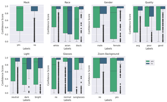
Figure A1.
Box plot of categorical labels vs. confidence scores for all image qualities, as qualitatively evaluated, using the augmented MobileNetv2 model. For each category and its labels, ‘mask’ and ‘no mask’ scores are plotted beside each other. The median is represented by the center line of each box while the upper and lower bounds represent the respective quartiles. Outliers are represented by diamond symbols.
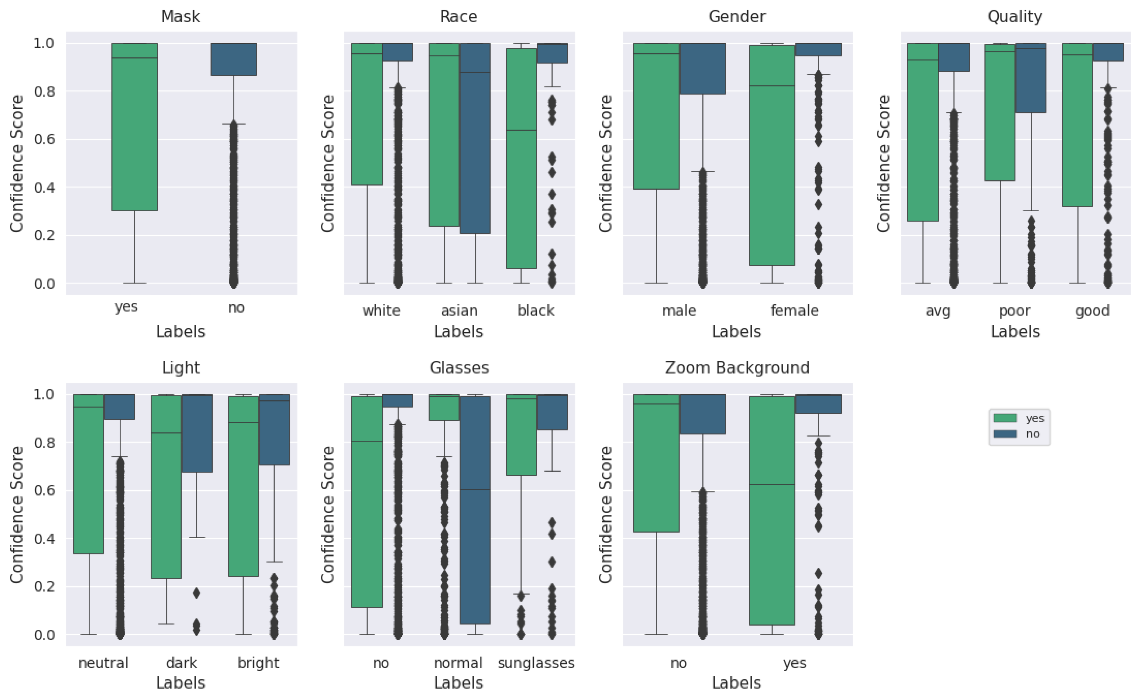
Figure A3 and Figure A4 show that the ‘mask’ images of ‘good’ quality were generally classified with higher accuracy and a higher confidence score. Moreover, the importance of quantitative quality labeling is apparent based on Figure A3 and Figure A4 that the distribution of the confidence score for the ‘mask’ label is significantly different for the qualitative quality label and the BRISQUE quality label. The performance on images filtered for ‘good’ quality via the BRISQUE metric is also notable as it is much poorer than that for the qualitative metric for the ‘no mask’ category, which is believed to be due to the greater number of ‘no mask’ images in the qualitatively labeled set (320) compared to the number of ‘no mask’ images in the BRISQUE quality set. Across all images (excluding the ‘other’ category), ‘no mask’ labeled images make up 46.28% of the data. In the ‘good’ (BRISQUE) quality category, they make up only 26.76% of the data. In the ‘good’ (qualitative) quality category, ‘no mask’ images make up 62.69% of the data. Therefore, the discrepancy can likely be attributed to the generally poorer performance of ‘no mask’ images and the lower number of images after filtering for quality. Although this is counter-intuitive as the training dataset was largely composed of photos of individuals not wearing masks, and one would expect higher performance on the same type of image, the images captured in the Zoom experiments are still of poorer quality and vary more in characteristics such as race than the training dataset, even when taking into account the Instagram data inclusion. In the hypothetical end application where images are being taken in a fixed location, we anticipate much better consistency in the image quality (fixed or slowly varying ambient conditions as well as a single camera of interest) and other controllable environmental factors.
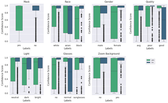
Figure A2.
Box plot of categorical labels vs. confidence scores for all image qualities, as evaluated via BRISQUE, using the augmented MobileNetv2 model. For each category and its labels, ‘mask’ and ‘no mask’ scores are plotted beside each other. The median is represented by the center line of each box while the upper and lower bounds represent the respective quartiles. Outliers are represented by diamond symbols. The primary difference between this plot and Figure A1 is the ‘Quality’ subplot, which shows the difference in the original subjective and the BRISQUE quantitative quality categories.
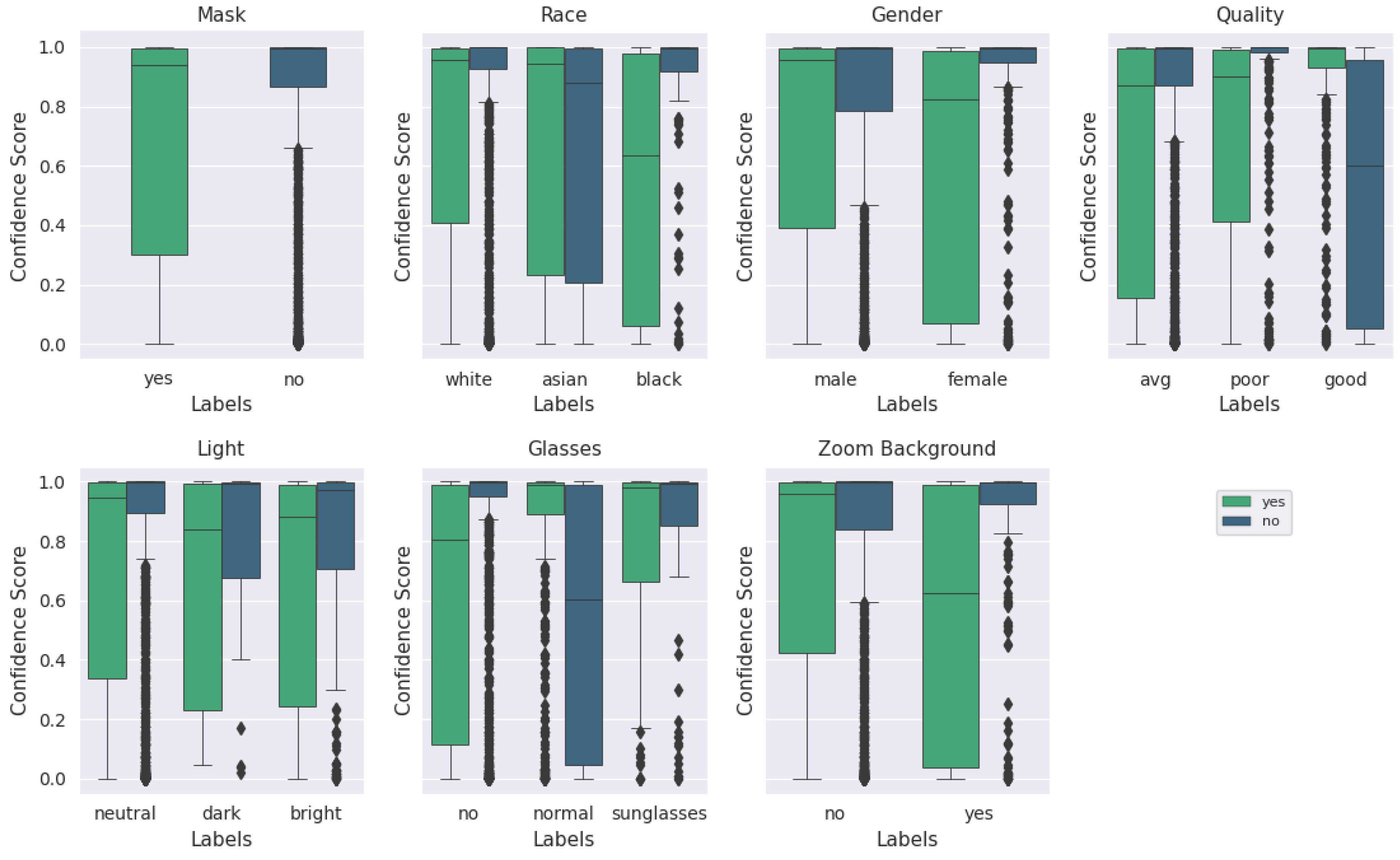
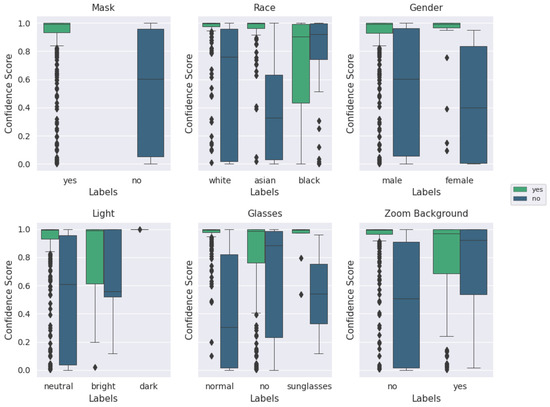
Figure A3.
Box plot of categorical labels vs. confidence scores for only good quality images, as evaluated via BRISQUE using the augmented MobileNetv2 model. For each category and its labels, ‘mask’ and ‘no mask’ scores are plotted beside each other. The median is represented by the center line of each box while the upper and lower bounds represent the respective quartiles. Outliers are represented by diamond symbols.
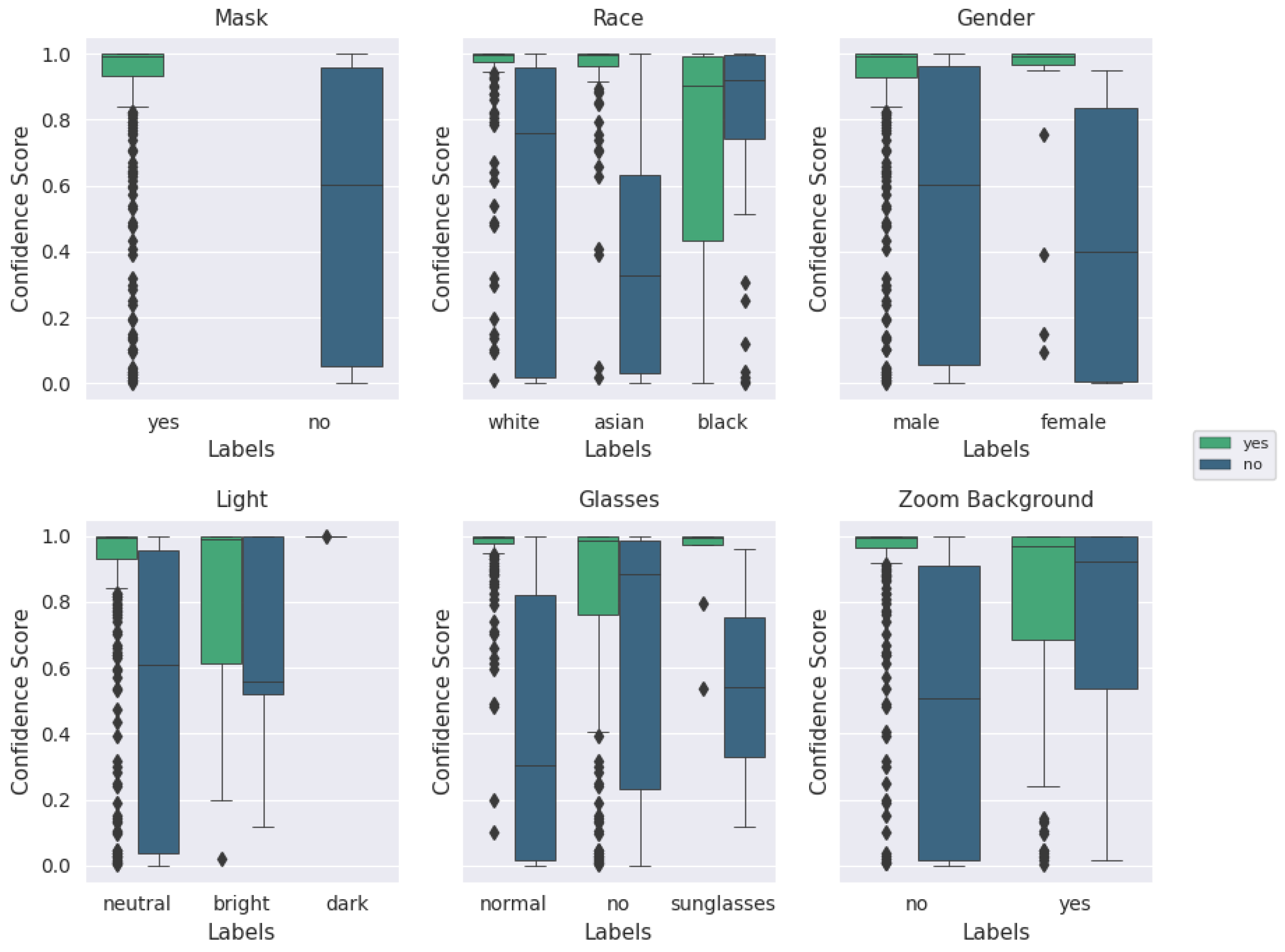
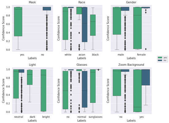
Figure A4.
Box plot of categorical labels vs. confidence scores for only good quality images, as qualitatively evaluated, using the augmented MobileNetv2 model. For each category and its labels, ‘mask’ and ‘no mask’ scores are plotted beside each other. The median is represented by the center line of each box while the upper and lower bounds represent the respective quartiles. Outliers are represented by diamond symbols.
References
- World Health Organization. Listings of WHO’s Response to COVID-19. Available online: https://www.who.int/news/item/29-06-2020-covidtimeline (accessed on 20 January 2020).
- Parker-Pope, T. The Scientist, the Air and the Virus. The New York Times, 30 June 2020. [Google Scholar]
- Biden, J. Executive Order on Promoting COVID-19 Safety in Domestic and International Travel. The White House, 21 January 2021. [Google Scholar]
- Biden, J. Executive Order on Protecting the Federal Workforce and Requiring Mask-Wearing. The White House, 20 January 2021. [Google Scholar]
- Lyu, W.; Wehby, G.L. Community Use Of Face Masks Furthermore, COVID-19: Evidence From A Natural Experiment Of State Mandates In The US: Study examines impact on COVID-19 growth rates associated with state government mandates requiring face mask use in public. Health Aff. 2020, 39, 1419–1425. [Google Scholar] [CrossRef]
- Bromwich, J.E. Fighting over Masks in Public Is the New American Pastime. The New York Times, 30 June 2020. [Google Scholar]
- Staff, C. Ventura County Sheriff: Face Mask Confrontation Caused Melee at Thousand Oaks Mall. CBS Los Angeles, 7 December 2020. [Google Scholar]
- Bar Attack Suspect Captured, Charged with Assault. Available online: https://abc13.com/bar-employee-assaulted-face-mask-josh-vaughan-grand-prize/8991178/ (accessed on 25 December 2020).
- Mahdavinejad, M.S.; Rezvan, M.; Barekatain, M.; Adibi, P.; Barnaghi, P.; Sheth, A.P. Machine learning for Internet of Things data analysis: A survey. Digit. Commun. Netw. 2018, 4, 161–175. [Google Scholar] [CrossRef]
- Gallagher, C. Masks No Obstacle for New NEC Facial Recognition System. Reuters, 7 July 2021. [Google Scholar]
- Nagpal, S.; Singh, M.; Singh, R.; Vatsa, M. Deep learning for face recognition: Pride or prejudiced? arXiv 2019, arXiv:1904.01219. [Google Scholar]
- Buolamwini, J.; Gebru, T. Gender shades: Intersectional accuracy disparities in commercial gender classification. In Proceedings of the Conference on Fairness, Accountability and Transparency, New York, NY, USA, 23–24 February 2018; PMLR: London, UK, 2018; pp. 77–91. [Google Scholar]
- Dodge, S.; Karam, L. Understanding how image quality affects deep neural networks. In Proceedings of the 2016 Eighth International Conference on Quality of Multimedia Experience (QoMEX), Lisbon, Portugal, 6–8 June 2016; IEEE: New York, NY, USA; pp. 1–6. [Google Scholar]
- Cho, S.W.; Baek, N.R.; Kim, M.C.; Koo, J.H.; Kim, J.H.; Park, K.R. Face detection in nighttime images using visible-light camera sensors with two-step faster region-based convolutional neural network. Sensors 2018, 18, 2995. [Google Scholar] [CrossRef] [Green Version]
- Klare, B.F.; Burge, M.J.; Klontz, J.C.; Vorder Bruegge, R.W.; Jain, A.K. Face Recognition Performance: Role of Demographic Information. IEEE Trans. Inf. Forensics Secur. 2012, 7, 1789–1801. [Google Scholar] [CrossRef] [Green Version]
- Acien, A.; Morales, A.; Vera-Rodriguez, R.; Bartolome, I.; Fierrez, J. Measuring the gender and ethnicity bias in deep models for face recognition. In Iberoamerican Congress on Pattern Recognition; Springer: Madrid, Spain, 2018; pp. 584–593. [Google Scholar]
- Srinivas, N.; Ricanek, K.; Michalski, D.; Bolme, D.S.; King, M. Face recognition algorithm bias: Performance differences on images of children and adults. In Proceedings of the IEEE/CVF Conference on Computer Vision and Pattern Recognition Workshops, Long Beach, CA, USA, 16–17 June 2019. [Google Scholar]
- Zafeiriou, S.; Zhang, C.; Zhang, Z. A survey on face detection in the wild: Past, present and future. Comput. Vis. Image Underst. 2015, 138, 1–24. [Google Scholar] [CrossRef] [Green Version]
- Yang, M.H.; Kriegman, D.J.; Ahuja, N. Detecting faces in images: A survey. IEEE Trans. Pattern Anal. Mach. Intell. 2002, 24, 34–58. [Google Scholar] [CrossRef] [Green Version]
- Taskiran, M.; Kahraman, N.; Erdem, C.E. Face recognition: Past, present and future (a review). Digit. Signal Process. 2020, 106, 102809. [Google Scholar] [CrossRef]
- Viola, P.; Jones, M. Robust real-time object detection. Int. J. Comput. Vis. 2001, 4, 4. [Google Scholar]
- Zhang, L.; Chu, R.; Xiang, S.; Liao, S.; Li, S.Z. Face detection based on multi-block LBP representation. In International Conference on Biometrics; Springer: Berlin/Heidelberg, Germany, 2007; pp. 11–18. [Google Scholar]
- Kadir, K.; Kamaruddin, M.K.; Nasir, H.; Safie, S.I.; Bakti, Z.A.K. A comparative study between LBP and Haar-like features for Face Detection using OpenCV. In Proceedings of the 2014 4th International Conference on Engineering Technology and Technopreneuship (ICE2T), Kuala Lumpur, Malaysia, 28–16 August 2014; pp. 335–339. [Google Scholar]
- Li, H.; Lin, Z.; Shen, X.; Brandt, J.; Hua, G. A convolutional neural network cascade for face detection. In Proceedings of the IEEE Conference on Computer Vision and Pattern Recognition, Boston, MA, USA, 7–12 June 2015; pp. 5325–5334. [Google Scholar]
- Zhang, K.; Zhang, Z.; Li, Z.; Qiao, Y. Joint face detection and alignment using multitask cascaded convolutional networks. IEEE Signal Process. Lett. 2016, 23, 1499–1503. [Google Scholar] [CrossRef] [Green Version]
- Jiang, H.; Learned-Miller, E. Face detection with the faster R-CNN. In Proceedings of the 2017 12th IEEE International Conference on Automatic Face & Gesture Recognition (FG 2017), Washington, DC, USA, 30 May–3 June 2017; IEEE: New York, NY, USA, 2017; pp. 650–657. [Google Scholar]
- Viola, P.; Jones, M. Rapid object detection using a boosted cascade of simple features. In Proceedings of the 2001 IEEE Computer Society Conference on Computer Vision and Pattern Recognition, CVPR 2001, Kauai, HI, USA, 8–14 December 2001; IEEE: New York, NY, USA, 2001; Volume 1, p. I. [Google Scholar]
- Freund, Y.; Schapire, R.E. A decision-theoretic generalization of on-line learning and an application to boosting. J. Comput. Syst. Sci. 1997, 55, 119–139. [Google Scholar] [CrossRef] [Green Version]
- Tieu, K.; Viola, P. Boosting image retrieval. Int. J. Comput. Vis. 2004, 56, 17–36. [Google Scholar] [CrossRef]
- Sandler, M.; Howard, A.; Zhu, M.; Zhmoginov, A.; Chen, L.C. Mobilenetv2: Inverted residuals and linear bottlenecks. In Proceedings of the IEEE Conference on Computer Vision and Pattern Recognition, Salt Lake City, UT, USA, 18–22 June 2018; pp. 4510–4520. [Google Scholar]
- He, K.; Zhang, X.; Ren, S.; Sun, J. Deep residual learning for image recognition. In Proceedings of the IEEE Conference on Computer Vision and Pattern Recognition, Las Vegas, NV, USA, 27–30 June 2016; pp. 770–778. [Google Scholar]
- Chen, Y.; Song, L.; He, R. Masquer hunter: Adversarial occlusion-aware face detection. arXiv 2017, arXiv:1709.05188. [Google Scholar]
- Wang, Z.; Wang, G.; Huang, B.; Xiong, Z.; Hong, Q.; Wu, H.; Yi, P.; Jiang, K.; Wang, N.; Pei, Y.; et al. Masked face recognition dataset and application. arXiv 2020, arXiv:2003.09093. [Google Scholar]
- Ge, S.; Li, J.; Ye, Q.; Luo, Z. Detecting masked faces in the wild with LLE-CNNs. In Proceedings of the IEEE Conference on Computer Vision and Pattern Recognition, Honolulu, HI, USA, 21–26 July 2017; pp. 2682–2690. [Google Scholar]
- Clark IV, W.H.; Hauser, S.; Headley, W.C.; Michaels, A.J. Augmentation of Real-World Data for Neural Network Based Automatic Modulation Classification. J. Def. Model. Simulation: Appl. Methodol. Technol. Spec. Issue 2021. accepted. [Google Scholar]
- Hao, D.; Zhang, L.; Sumkin, J.; Mohamed, A.; Wu, S. Inaccurate Labels in Weakly-Supervised Deep Learning: Automatic Identification and Correction and Their Impact on Classification Performance. IEEE J. Biomed. Health Inf. 2020, 24, 2701–2710. [Google Scholar] [CrossRef]
- Mittal, A.; Moorthy, A.K.; Bovik, A.C. No-reference image quality assessment in the spatial domain. IEEE Trans. Image Process. 2012, 21, 4695–4708. [Google Scholar] [CrossRef]
- Moorthy, A.K.; Bovik, A.C. Blind Image Quality Assessment: From Natural Scene Statistics to Perceptual Quality. IEEE Trans. Image Process. 2011, 20, 3350–3364. [Google Scholar] [CrossRef] [PubMed]
- Saad, M.A.; Bovik, A.C.; Charrier, C. Blind image quality assessment: A natural scene statistics approach in the DCT domain. IEEE Trans. Image Process. 2012, 21, 3339–3352. [Google Scholar] [CrossRef]
- Paszke, A.; Gross, S.; Massa, F.; Lerer, A.; Bradbury, J.; Chanan, G.; Killeen, T.; Lin, Z.; Gimelshein, N.; Antiga, L.; et al. PyTorch: An imperative style, high-performance deep learning library. In Advances in Neural Information Processing Systems 32; Neural Information Processing Systems Foundation: Vancouver, BC, Canada, 2019; pp. 8026–8037. [Google Scholar]
- Bradski, G. OpenCV. Open Source Computer Vision Library. In Dr. Dobb’s Journal of Software Tools; 2000; Available online: http://ftp.math.utah.edu/pub/tex/bib/toc/dr-dobbs-2000.html (accessed on 24 September 2021).
- US Department of Health and Human Services. 45 CFR 46—PROTECTION OF HUMAN SUBJECTS—Subpart A—Basic HHS Policy for Protection of Human Research Subjects; Code of Federal Regulations Authority, 5; US Department of Health and Human Services: Washington, DC, USA, 2019. [Google Scholar]
- Branco, P.; Torgo, L.; Ribeiro, R.P. A survey of predictive modeling on imbalanced domains. ACM Comput. Surv. (CSUR) 2016, 49, 1–50. [Google Scholar] [CrossRef]
- Albiero, V.; Chen, X.; Yin, X.; Pang, G.; Hassner, T. img2pose: Face Alignment and Detection via 6DoF, Face Pose Estimation. arXiv 2020, arXiv:2012.07791. [Google Scholar]
- Schuckers, S. Presentations and attacks, and spoofs, oh my. Image Vis. Comput. 2016, 55, 26–30. [Google Scholar] [CrossRef] [Green Version]
- Ramachandra, R.; Busch, C. Presentation attack detection methods for face recognition systems: A comprehensive survey. ACM Comput. Surv. (CSUR) 2017, 50, 1–37. [Google Scholar] [CrossRef]
- Zoom. Video Conferencing, Web Conferencing, Webinars, Screen Sharing—Zoom. 2021. Available online: https://zoom.us/ (accessed on 2 March 2021).
- Kluyver, T.; Ragan-Kelley, B.; Pérez, F.; Granger, B.; Bussonnier, M.; Frederic, J.; Kelley, K.; Hamrick, J.; Grout, J.; Corlay, S.; et al. Jupyter Notebooks—A publishing format for reproducible computational workflows. In Positioning and Power in Academic Publishing: Players, Agents and Agendas; Loizides, F., Schmidt, B., Eds.; IOS Press: Amsterdam, The Netherlands, 2016; pp. 87–90. [Google Scholar]
- Xiao, T.; Xia, T.; Yang, Y.; Huang, C.; Wang, X. Learning from massive noisy labeled data for image classification. In Proceedings of the IEEE Conference on Computer Vision and Pattern Recognition, Boston, MA, USA, 7–12 June 2015; pp. 2691–2699. [Google Scholar]
- Phillips, P.J.; Beveridge, J.R.; Bolme, D.S.; Draper, B.A.; Givens, G.H.; Lui, Y.M.; Cheng, S.; Teli, M.N.; Zhang, H. On the existence of face quality measures. In Proceedings of the 2013 IEEE Sixth International Conference on Biometrics: Theory, Applications and Systems (BTAS), Arlington, VA, USA, 29 September–2 October 2013; IEEE: New York, NY, USA, 2013; pp. 1–8. [Google Scholar]
- Logitech. Logitech C922 Pro Stream 1080p Webcam + Capture Software. Available online: https://www.logitech.com/en-us/products/webcams/c922-pro-stream-webcam.960-001087.html (accessed on 20 October 2021).
- Perez, F.; Granger, B.E. Project Jupyter: Computational narratives as the engine of collaborative data science. Retrieved Sept. 2015, 11, 108. [Google Scholar]
- Choi, H.; Geeves, M.; Alsalam, B.; Gonzalez, F. Open source computer-vision based guidance system for UAVs on-board decision making. In Proceedings of the 2016 IEEE Aerospace Conference, Big Sky, MT, USA, 5–12 March 2016; IEEE: New York, NY, USA, 2016; pp. 1–5. [Google Scholar]
- Patchava, V.; Kandala, H.B.; Babu, P.R. A smart home automation technique with raspberry pi using iot. In Proceedings of the 2015 International Conference on Smart Sensors and Systems (IC-SSS), Bangalore, India, 21–23 December 2015; IEEE: New York, NY, USA, 2015; pp. 1–4. [Google Scholar]
- Worsley, K.; Eddin, A.S.; Xiong, J.; Hwu, W.m.; El-Hadedy, M. Performance Analysis of Computer Vision with Machine Learning Algorithms on Raspberry Pi 3. In Proceedings of the Future Technologies Conference, Vancouver, Canada, 5–6 November 2020; Springer: Berlin/Heidelberg, Germany, 2020; pp. 216–232. [Google Scholar]
- Brahmbhatt, S. Embedded computer vision: Running OpenCV programs on the Raspberry Pi. In Practical OpenCV; Springer: Berlin/Heidelberg, Germany, 2013; pp. 201–218. [Google Scholar]
- Clayton, C. Virginia Department of Health Announces Launch of QR Codes to Verify COVID-19 Vaccination Status; Virginia Department of Health: Henrico, VA, USA, 2021. [Google Scholar]
- Cabrera, M. Coffee and Croissant in a French Cafe? You’ll Need a COVID Pass for That. Reuters, 21 August 2021. [Google Scholar]
- Project, T.C. SMART Health Card Verifier App. 2021. Available online: https://thecommonsproject.org/smart-health-card-verifier (accessed on 10 October 2021).
- Williamson, D.F.; Parker, R.A.; Kendrick, J.S. The box plot: A simple visual method to interpret data. Ann. Intern. Med. 1989, 110, 916–921. [Google Scholar] [CrossRef] [PubMed]
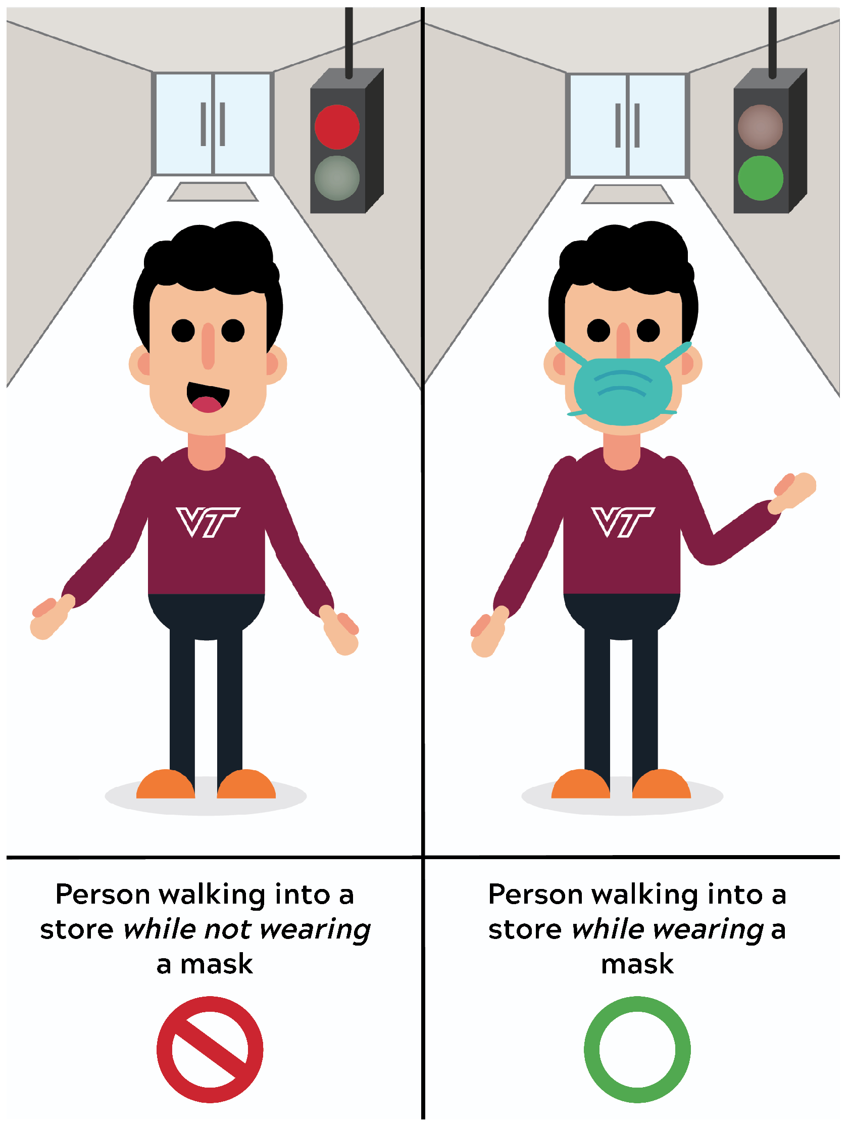


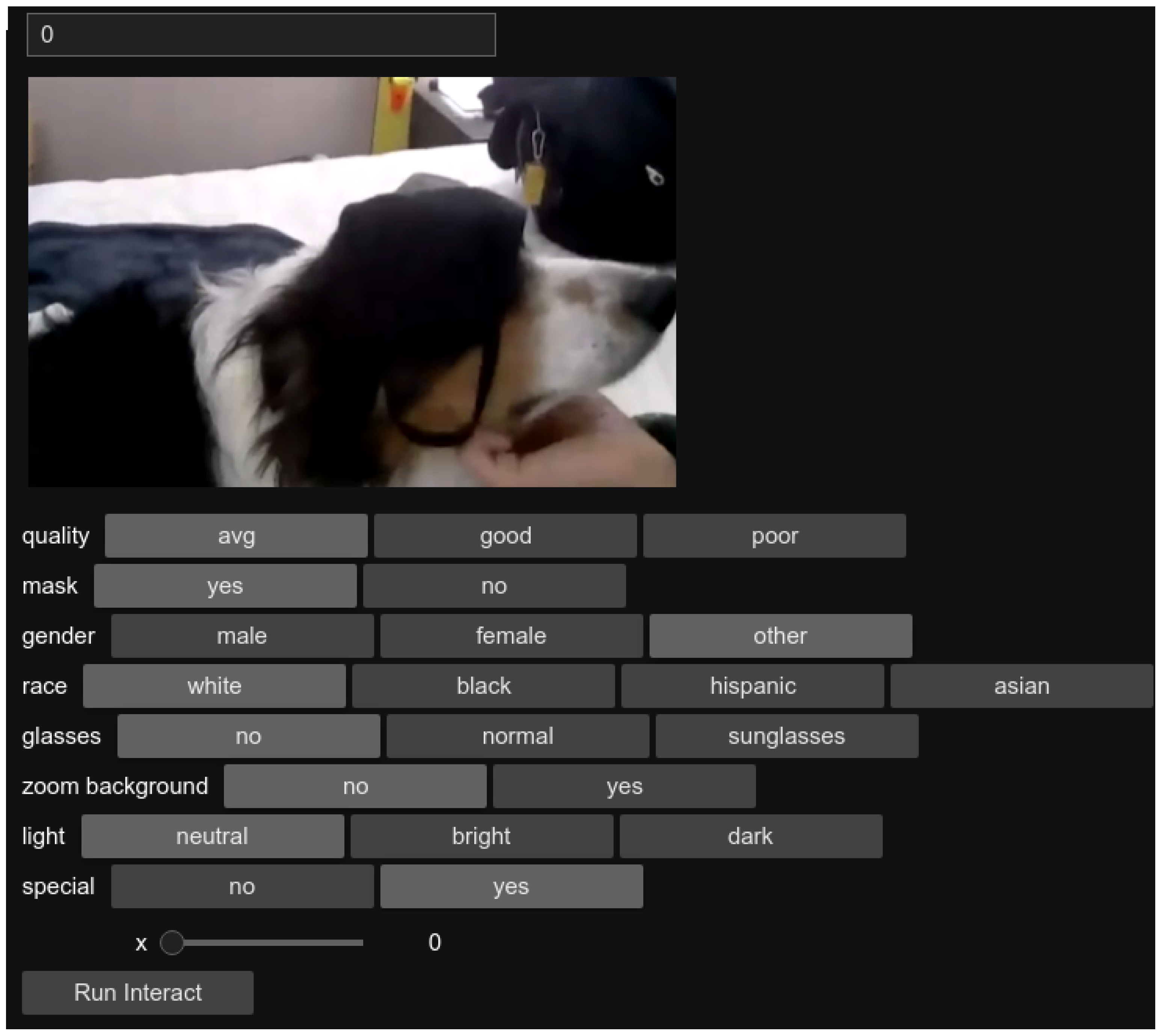
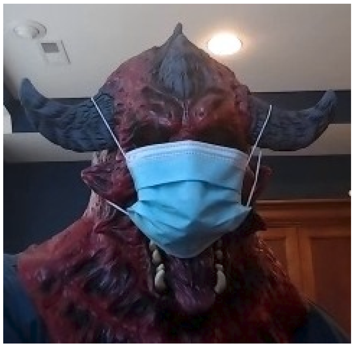
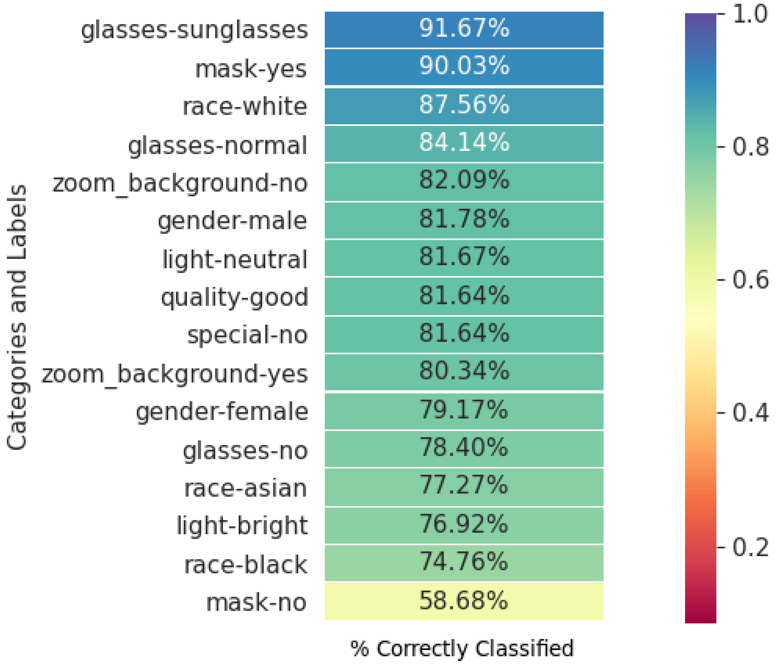

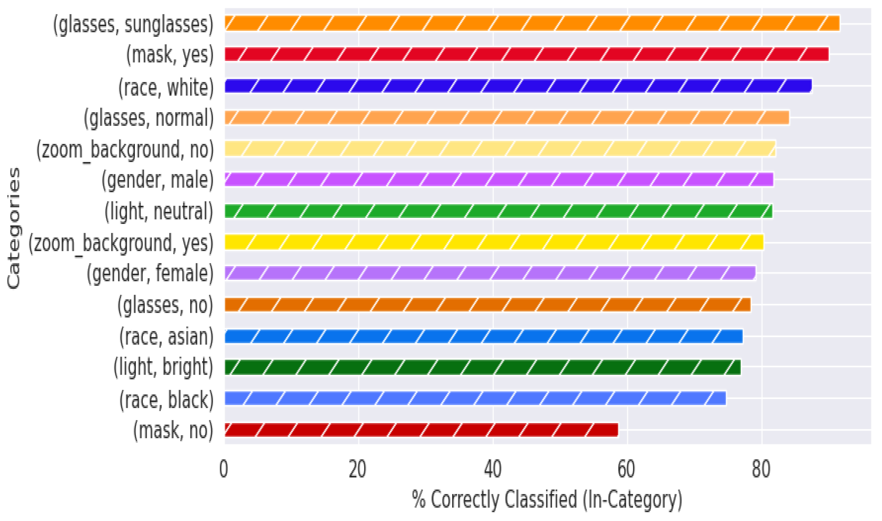
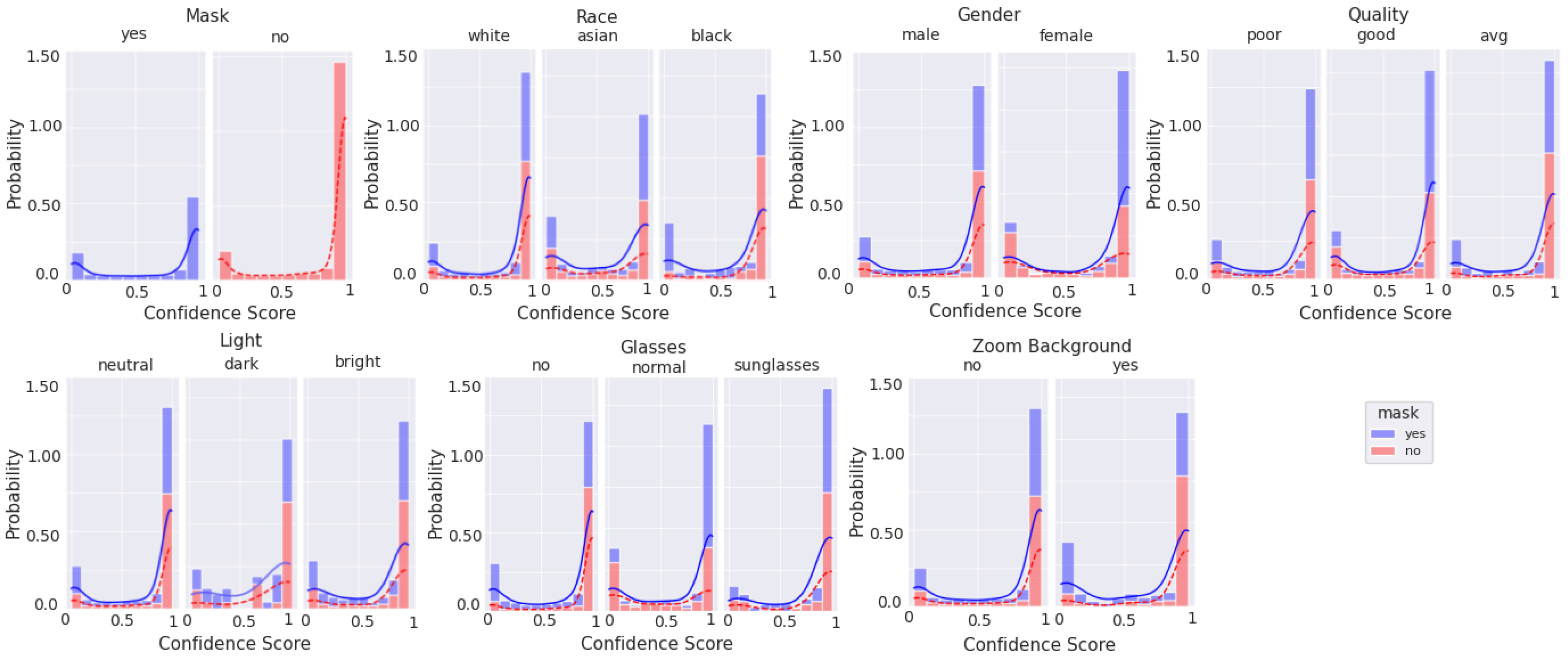

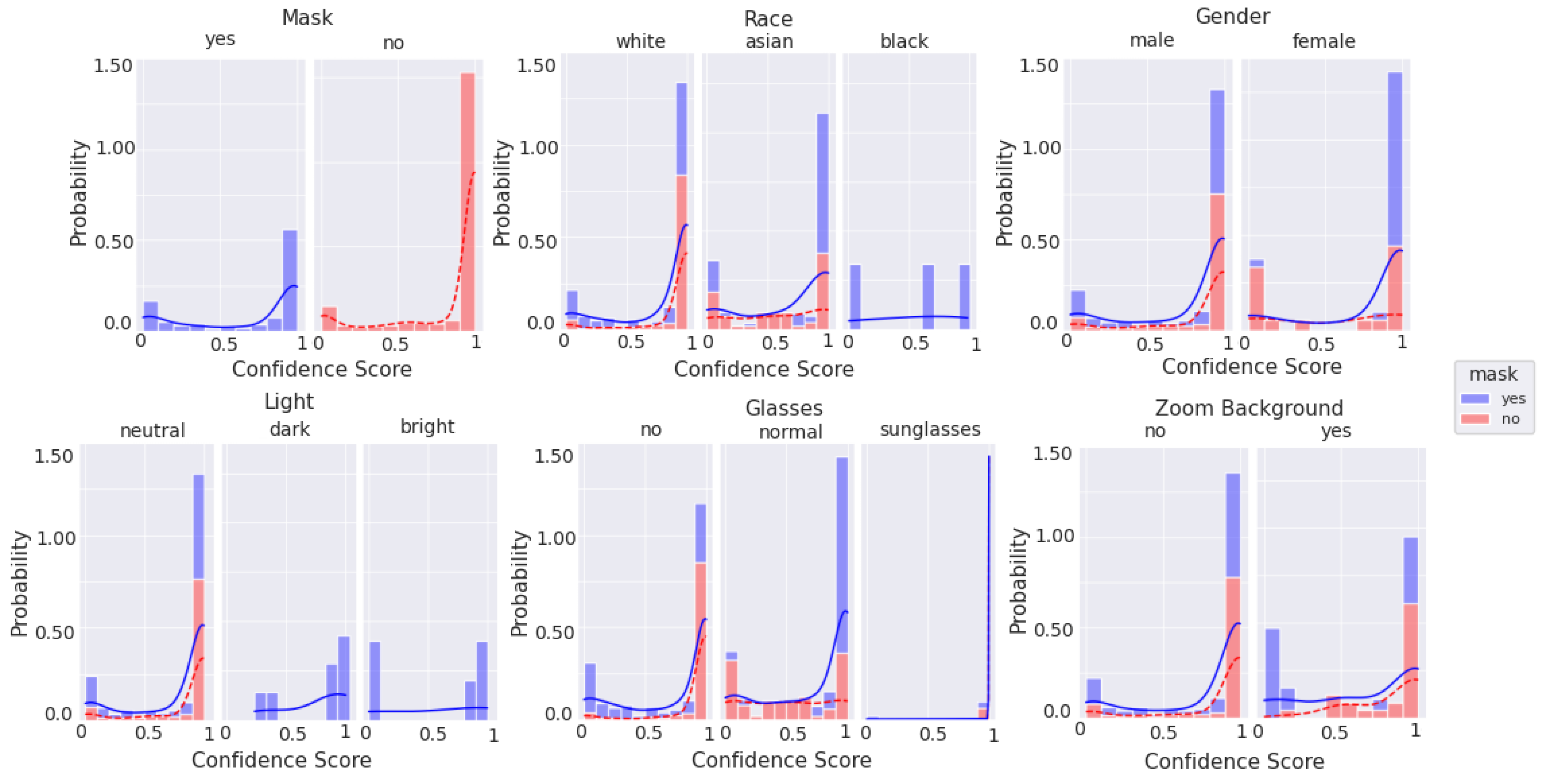
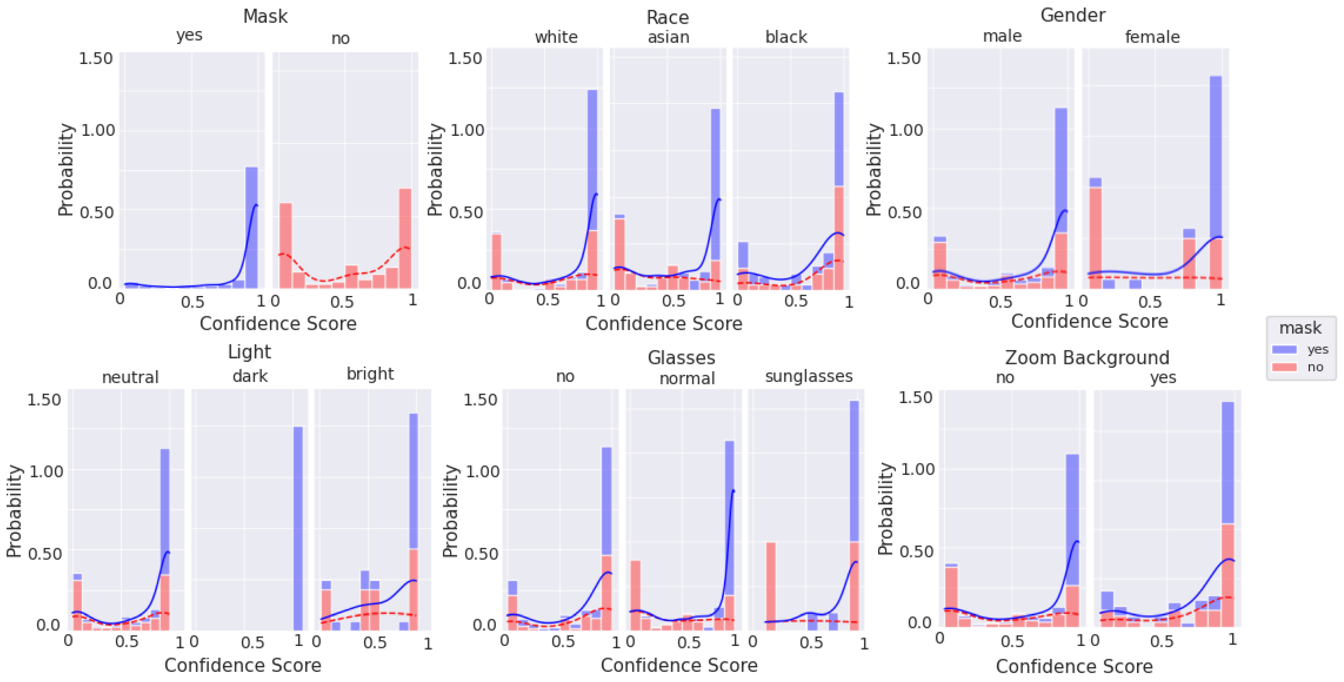

Publisher’s Note: MDPI stays neutral with regard to jurisdictional claims in published maps and institutional affiliations. |
© 2021 by the authors. Licensee MDPI, Basel, Switzerland. This article is an open access article distributed under the terms and conditions of the Creative Commons Attribution (CC BY) license (https://creativecommons.org/licenses/by/4.0/).