Article

Landslide Susceptibility Assessment Based on a Quantitative Continuous Model: A Case Study of Wanzhou

Nanjing Center of Geological Survey, China Geological Survey, Nanjing 210016, China
*
Author to whom correspondence should be addressed.
GeoHazards 2025, 6(3), 48; https://doi.org/10.3390/geohazards6030048
Submission received: 23 July 2025 / Revised: 21 August 2025 / Accepted: 25 August 2025 / Published: 26 August 2025

Abstract

Landslide susceptibility assessment constitutes a pivotal method of preventing and reducing losses caused by geological disasters. However, traditional models are often influenced by subjective grading factors, which can result in unscientific and inaccurate assessment outcomes. In this study, we thoroughly analyze various landslide causative factors, including geological, topographical, hydrological, and environmental components. A quantitative continuous model was employed, with methods such as frequency ratio (FR), cosine amplitude (CA), information value (IV), and certainty factor (CF) being applied in order to assess the landslide susceptibility of the Wanzhou coastline in the Three Gorges Reservoir area. The results were then compared with methods such as Bias-Standardised Information Value (BSIV), Support Vector Machine (SVM), Random Forest (RF), and Gradient Boosted Decision Tree (GBDT). This process led to the following key conclusions: (1) Most landslide susceptibility zones are predominantly banded and clustered on both sides of the Dewuidu River, particularly along the left bank of the Yangtze River from Dewuidu Town to Wanzhou City, as well as in the main urban area of Wanzhou. Clusters of the Yangtze River mainstem and surrounding towns characterize these areas. (2) The enhanced statistical analysis model shows a notable increase in sensitivity to landslides, achieving an Area Under the Curve (AUC) of 0.8878 for the IV model—an improvement of 0.0639 over the traditional BSIV model. This enhancement aligns closely with machine learning capabilities, and the spatial results obtained are more continuous. (3) By substituting manual grading with a quantitative continuous model, we achieve a balance between interpretability and computational efficiency. These findings lay a scientific foundation for the prevention and management of geological disasters in Wanzhou and provide valuable insights for comparable regions undertaking landslide susceptibility assessments.

1. Introduction

Landslides represent a prevalent form of geological hazard, precipitated by variables including precipitation, seismic activity, and anthropogenic influence [1]. The consequences of such actions may include fatalities, property damage, and the impairment of transportation infrastructure and the environment [2]. A comprehensive understanding of the mechanisms, impacts, and mitigation strategies of landslides is imperative for sustainable development and disaster risk management [3]. Wanzhou, located in Chongqing’s Three Gorges Reservoir Area, is known for its frequent landslides, which are attributed to its complex natural geography and geological environment [4]. Landslide susceptibility (LS) refers to the likelihood of landslide disasters occurring in a specific area that is affected by geological conditions related to disaster prevention [5]. Landslide susceptibility assessment (LSA) is a tool utilized to evaluate the probability of landslides occurring, thereby providing a foundation for the prevention of geological disasters [6]. Initially, LSA was predominantly reliant on field surveys and the interpretation of airborne imagery, with the precision of the evaluation outcomes contingent on the intricacy of the field surveys and the expertise of the analysts [7]. The advent of Remote Sensing (RS) and Geographic Information System (GIS) has facilitated the application of numerous models (e.g., statistical analysis, mathematical statistics, machine learning) in LSA research and applications, thereby enhancing the efficacy of such research and applications [8,9]. Qualitative analysis methods based on experts’ experience (e.g., hierarchical analysis, subjective weighting) are intensely subjective and less objective in assigning weights [10,11]. The application of machine learning methods for quantitative analysis, including Artificial Neural Networks (ANN), Random Forest (RF), Deep Learning (DL), and Logistic Regression (LR), necessitates frequent iterative operations and parameter adjustments, thereby rendering the operation relatively complex [12,13,14,15,16]. Statistical analyses are favored by researchers for their simplicity and are relatively widely used, such as Information Value (IV), Certainty Factor (CF), Frequency Contrast (FC), and Weight of Evidence (WOE) [17,18,19,20,21]. However, implementing the statistical analysis method involves classifying or grading the geohazard impact factors, and determining the number of factors to be graded and their boundaries is subjective, which affects the model’s application [16]. Therefore, to improve the accuracy of statistical analysis methods for evaluating geohazard susceptibility, this study first used a continuous model for grading factors, then applied the Frequency Ratio (FR), Cosine Amplitude (CA), CF, and IV models to obtain LS results. These results were compared with those from Bias-Standardized Information Value (BSIV), RF, Support Vector Machine (SVM), and Gradient Boosting Decision Tree (GDBT), which have demonstrated better application effects, to analyze prediction accuracy and effectiveness. The research objectives are: (1) Establishing a quantitative, continuous model to address landslide causative factors and eliminate the subjectivity and discontinuity inherent in manual scoring systems; (2) Systematically comparing the performance of this improved method (when applied to FR, CA, CF and IV models) with that of traditional BSIV models and machine learning models (SVM, RF and GBDT) in terms of prediction accuracy and spatial consistency; (3) To generate a reliable and highly accurate landslide susceptibility map for Wanzhou that can inform local geological disaster prevention and risk management strategies.

2. Materials

2.1. Study Area

The study area is located in the Wanzhou District of Chongqing, China, and stretches 5 km along both banks of the Yangtze River (Figure 1). Encompassing 923.56 km2, the terrain features elevations that range from 21 m to 1429 m above sea level, showcasing a characteristic alpine landscape interspersed with low valleys [4]. The study area exhibits a complex geological structure and stress field, primarily composed of Jurassic and Triassic strata that date back approximately 230 to 137 million years [22]. Mudstone, shale, siltstone, feldspathic sandstone, quartz sandstone, limestone, and dolomite are all essential types of bedrock. This research area unquestionably has a typical subtropical climate, characterized by warm and humid conditions and distinct four seasons. Annual precipitation is unevenly distributed, with the majority falling from May to September (71.28% of the total) [23]. In this area, geological hazards such as avalanches, landslides and bank failures are primarily located in urban areas with high population concentration and dense housing, they may result in major disasters and accidents when triggered by factors such as extreme rainstorms and rising and falling water levels in reservoirs, thus restricting the development of the local economy to a certain extent [24].

2.2. Data Source

Concerning previous related studies, a total of 18 landslide causative factors were selected from four primary categories, including: geological (Engineered Rock Group), topographic (Elevation, Slope, Slope Height, Aspect, Profile Curvature, Plain Curvature, Terrain Roughness Index (TRI), Terrain Surface Texture (TST), and Terrain Position Index (TPI)), hydrological (Distance to River, Valley Depth, and Terrain Wetness Index (TWI)), and environmental (Rainfall, Normalized Vegetation Index (NDVI), Normalized Water Body Index (NDWI), Earthquake Magnitude and Land Use) in four categories, with each factor shown in Figure 2. The detailed factor information and extraction methods are presented in Table 1.

2.3. Data Preprocessing

To ensure spatial consistency and comparability among all landslide causative factors, systematic preprocessing was conducted on the raw data, including the following steps:
Data Cleaning and Missing Value Handling: All raster and vector datasets were inspected for missing values, which were either removed or interpolated. Rainfall data from meteorological stations were spatially interpolated using the IDW method, while earthquake data were gap-filled using the Kriging interpolation module.
Spatial Resolution Unification: All factor datasets were resampled to a uniform resolution of 30 m × 30 m to ensure spatial consistency.
Coordinate System Unification: All data were reprojected to a common coordinate system (WGS_1984_UTM_Zone_49N) to facilitate spatial overlay analysis.
Normalization: Continuous factors (e.g., elevation, slope) were normalized to the range [0, 1] using min-max normalization to eliminate scale effects.
All preprocessing steps were performed in ArcGIS 10.8, QGIS 3.4, SAGA 2.0.3, and ENVI 5.5.

3. Methods

The methodology of this study consists of three main steps (Figure 3):
First, data collection and pre-processing were conducted. We collected and processed data related to the study area, including regional landslide data and data on geological, topographical, hydrological, and environmental factors. We then carried out the necessary pre-processing of the data to select the most appropriate factors as inputs for the model.
Second, the model was used to assess the LS. The FR, CA, CF, IV, IBSIV, SVM, RF, and GDBT models were used to obtain the LS evaluation results. Four of these, FR, CA, CF, and IV, are obtained based on continuous model factor processing.
Finally, we performed a comparative analysis of model performance. We analyzed the pros and cons of statistical analysis methods using continuous models versus traditional and machine learning methods by comparing the LS results produced by different models.

3.1. Landslide Susceptibility Evaluation Models

3.1.1. Information Value (IV)

The information value model enables probabilistic predictions by calculating the information entropy of each factor and is therefore widely used in landslide susceptibility assessments [32]. When the information value is negative, the smaller the value, the lower the likelihood of a landslide disaster. Conversely, the greater the informativeness value, the higher the probability of geological disasters. Specifically, the formula for calculating the informativeness value of a factor is as follows:
I V i , j = l n p ( L | F i , j ) p L , F i
where I V i , j is the amount of information provided by level j of the landslide evaluation factor I V i ; it is assumed that there is a factor ( F ) level and a landslide ( L ) level for landslide susceptibility analysis. p L , F i represents the conditional F i ‘probability given L’, i.e., the a priori probability of landslide occurrence in the study area, which is obtained by dividing the number of landslide units in the study area by the total number of evaluation units; p ( L | F i , j ) is the conditional probability given ‘conditional probability given L’, the conditional probability of the occurrence of a landslide in the study area under the j classification. LS can be obtained by summing the informative values of all factors.

3.1.2. Frequency Ratio (FR)

Frequency Ratio quantify the sensitivity of a factor class to landslides using a comparison between conditional probabilities p L , F i and p ( L | F i , j ) [20]. Specifically, the FR of a characteristic interval is defined as:
F R i , j = p ( L | F i ) p ( L | F i , j )
Larger FR indicates higher landslide susceptibility, while smaller FR indicates lower susceptibility.

3.1.3. Certainty Factor (CF)

The deterministic factor approach also utilizes the exact conditional probabilities, as do the frequency ratio and informativeness approaches. The difference is that instead of simply comparing p L , F i and p ( L | F i , j ) , the deterministic factor approach derives a parameter called the ‘Certainty Factor (CF)’ through a more complex comparison relationship [33]. This parameter was initially proposed by Shortliffe and Buchanan and modified by Heckerman [34,35]. The deterministic factor (CF) of is defined as:
C F i , j = p ( L | F i , j ) p ( L | F i ) p ( L | F i , j ) · [ 1 p ( L | F i ) ]   p ( L | F i , j ) p ( L | F i ) p ( L | F i , j ) p ( L | F i ) p ( L | F i ) · [ 1 p ( L | F i , j ) ]   p ( L | F i , j ) p ( L | F i )
The value of the deterministic factor ranges from (−1, 1), when C F i , j is positive, it indicates a higher likelihood of landslide. The larger the value of the deterministic factor, the higher the landslide sensitivity.
It is important to note that deterministic factors do not lend themselves to simple superposition by summation. Suppose there exist two factors F1 and F2, and their corresponding deterministic factors are CF1 and CF2 at a particular location. At this point, the combined deterministic factor of the two factors can be calculated according to the following rule:
C F 1 + C F 2 = C F 1 + C F 2 C F 1 C F 2 ,   C F 1 ,   C F 2 0 C F 1 + C F 2 1 m i n ( C F 1 , C F 2 ) ,   C F 1 C F 2 < 0 C F 1 + C F 2 + C F 1 C F 2 ,   C F 1 ,   C F 2 < 0

3.1.4. Cosine Amplitude (CA)

CA is used to measure the similarity between two or more datasets [36]. Assuming the existence of two vectors V 1 = v 11 , v 12 , , v 1 N and V 2 = v 21 , v 22 , , v 2 N , the cosine amplitude (CA) is defined as:
C A V 1 V 2 = k = 1 N v 1 k v 2 k k = 1 N v 1 k 2 k = 1 N v 2 k 2
where C A V 1 V 2 is the cosine amplitude, which represents the strength of the relationship between V 1 and V 2 .
In the landslide susceptibility analysis, V 1 is a vector recording the occurrence of landslides and V 2 is a vector of the presence of factor categories, are both vectors of the total number of grid cells in the study area and for F i , j , the cosine amplitude (CA) is given by the following equation according to Equation (5):
C A i , j = N L F i , j N L N F i , j = N L F i , j N F i , j N L F i , j N L = p ( L | F i , j ) p ( F i , j | L )
In landslide susceptibility analysis based on fuzzy set theory, cosine amplitude is used as the affiliation value (propensity value) of the factor categories and LS is calculated by directly summing the cosine amplitudes of all the factors [37].

3.1.5. Bias-Standardized Information Value (BSIV)

Due to the varying contributions of different classes of the same factor to landslide formation, the BSIV model is employed to normalize the information value of the evaluation factors. This prevents the enhancement of high information values and the degradation of low information values, providing a more accurate representation of the contribution of each factor to different classes within various categories in the comprehensive analysis [38]. The calculation formula is as follows:
B S I V i , j = l n p ( L | F i , j ) p L , F i μ I V i , j σ I V i , j
where μ I V i , j and σ I V i , j are the mean and standard deviation of the informativeness values, respectively.

3.1.6. Support Vector Machine (SVM)

SVM is a generalized classifier that uses a supervised learning model for binary classification [39]. Due to its ability to efficiently process high-dimensional data and deal with nonlinear classification problems, it is commonly used for landslide susceptibility prediction [40]. The objective is to identify a classification hyperplane that meets the required classification accuracy standards while simultaneously maximizing the area on both sides, thereby attaining optimal data classification.
The penalty factor C for the SVM model was set to 1.0, and the radial basis function was selected. The gamma coefficient was set to ‘scale’. The output of the Support Vector Machine (SVM) for the LS is typically the signed distance of a pixel from the decision hyperplane [39]. While not a direct probability, higher (more positive) values are indicative of higher confidence in belonging to the landslide class, which is interpreted as higher LS.

3.1.7. Random Forest (RF)

RF is an integrated tree model that uses the Classification and Regression Tree (CART) algorithm as a classifier [41]. In the RF model, M new training sets are generated by randomly selecting N original samples (with the exact dimensions as N), and then a decision tree model is constructed. The final result is obtained by combining the classification and prediction information from multiple decision trees through a voting mechanism, with the majority decision prevailing [42].
For the RF model, the number of random forest trees was set to 100, and the maximum depth to 3. For a classification task (landslide/non-landslide), the RF model can output the predicted class or the class probability. In this study, the probability of a pixel being classified as a landslide (ranging from 0 to 1) is used as the continuous susceptibility index.

3.1.8. Gradient Boosting Decision Tree (GBDT)

GBDT utilizes the CART algorithm as its base classifier and an additive model to reduce sample residuals generated during training progressively [43]. Predictions and residuals are obtained from the first leaf of the decision tree in the dataset, and subsequent decision trees are trained based on the projections and residuals from the previously trained trees. After each iteration, a new composite model is built to decrease the residuals. During the iterative process, all trees are optimized by minimizing the loss function. Similarly to RF, the GBDT model outputs the predicted probability of landslide occurrence (0 to 1) for each pixel, which serves as a highly optimized susceptibility index.
In the GDBT model, all trees are interrelated, and creating a new tree each time can reduce the residual of previous samples. The model is robust against missing data and outliers, is not easily affected by extreme values, and can handle high-dimensional sparse data. The GBDT model has demonstrated outstanding predictive accuracy in various machine learning and practical applications.

3.2. Quantitative Continuum Model

The statistical analysis method based on the continuous model is applied to evaluate geological disaster susceptibility, comprising the following three steps (Step 2 in Figure 3):
(1)
Normalized factor value
The factor values of geological disaster impact factors are to be normalized with continuous values. In other words, a linear mapping is required that maps continuous values to a range between 0 and 1.
(2)
Precision Set
The parameter ‘precision’ defines the number of decimal places to get the same normalized factor value. For example, when ‘precision’ is 3, the normalized factor values 0.11656 and 0.11682 will both become the same normalized factor value 0.117, and there will be up to 1001 identical normalized factor values. The application of ‘precision’ can reduce the amount of computation by eliminating the need for identical normalized values.
A ‘bin’ is created for each normalized factor value, centered around that value, with its width determined by the ‘bin width’ parameter, which can be understood as the width of each factor level in traditional methods.
(3)
Generation LS Layer
Finally, the empirical conditional probabilities and favorability values for each factor are obtained, based on which a favorability layer for that factor with factor values can be generated based on the methods in Section 3.1.1, Section 3.1.2, Section 3.1.3 and Section 3.1.4.
The generation of LS is controlled by ‘bin width’ and ‘precision’. Lower values of ‘precision’ (e.g., 2 or 3) have been shown to result in the excessive discretization of continuous data, while higher values of ‘precision’ (e.g., 5 or 6) have been demonstrated to increase both the number of unique values and the computational load [16]. A small ‘bin width’ can result in unstable and noisy calculated statistical metrics. Conversely, a big ‘bin width’ can result in the data becoming too smooth, thereby undermining the purpose of the continuous model. Refer to the relevant research when considering both computational efficiency and accuracy [44]. For the implementation of the statistical analysis model, the parameters ‘precision’ and ‘bin width’ were set to 4 and 0.1, respectively.

3.3. Accuracy of Models

The accuracy of the model is validated using the success rate method, which is represented by the ROC (Receiver Operating Characteristic) curve [45]. The ROC curve defines the false positive rate (FPR) on the X-axis and the actual positive rate (TPR) on the Y-axis. FPR is defined as the rate of false positives among all actual negative samples, and TPR is the rate of true positives among all actual positive samples. The greater the proximity of the curve to the upper left corner, the more precise the results. The area under the curve is referred to as the AUC (Area Under the Curve), and an AUC closer to 1 indicates a more successful model application [46].
The landslide sample data were divided into training and test sample sets in a 7:3 ratio. The performance metrics, including the FPR and TPR, were evaluated on the independent test set in order to ensure an unbiased assessment of the model’s predictive capability.

4. Results

4.1. Factor Selection

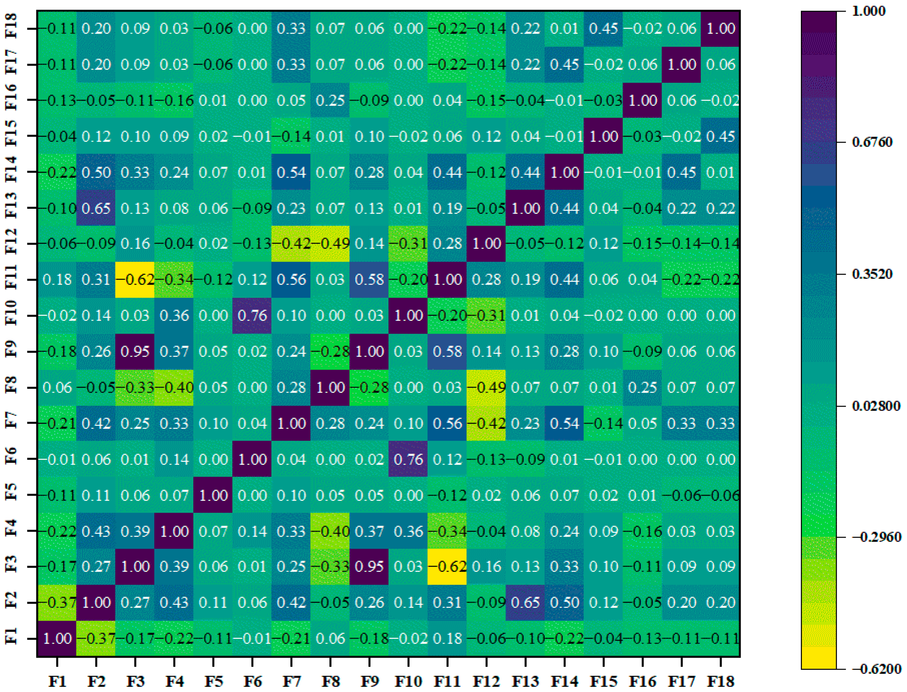
Factor selection was performed using Pearson correlation coefficients for the 18 landslide causative factors (Figure 4). Colors trending towards blue indicate positive correlations, while colors trending towards yellow indicate negative correlations. The intensity of the color indicates the strength of the correlation: larger dark values indicate stronger correlations, while lighter colors indicate weaker ones. For this study, 13 factors were selected as input data for the LS evaluation model: Engineered rock group, Slope, Slope height, Aspect, TST, TPI, Valley depth, Distance to river, Rainfall, NDVI, NDWI, Earthquake magnitude, and Land use. The correlation coefficients for these factors ranged from −0.5 to +0.5.

4.2. Landslide Susceptibility Results

The SVM, RF, and GDBT models were implemented using the scikit-learn Python library (1.4.0). Then, the landslide sample data were divided into training and test sample sets in a 7:3 ratio, which were used to fit the machine learning model. The four regional susceptibility predictions (FR, CA, CF, and IV) were then obtained using the continuous model optimization method. BSIV is based on the traditional factor grading method.
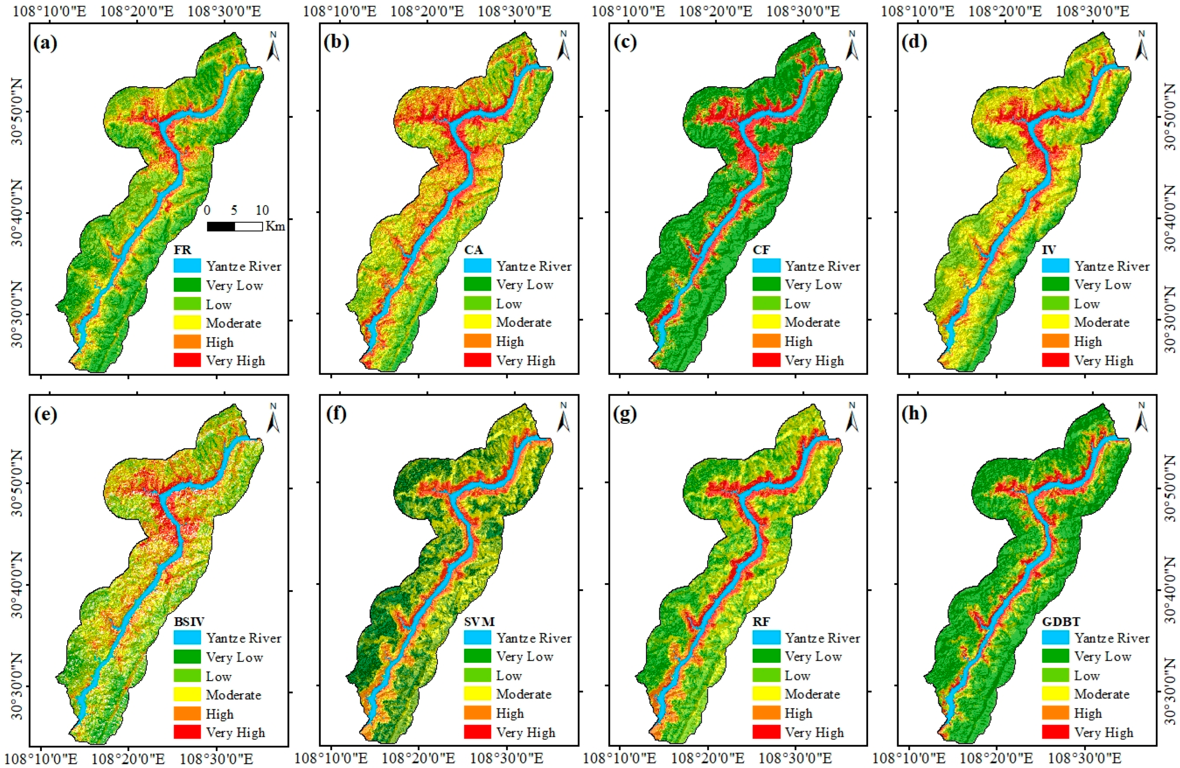
According to the distribution characteristics of the LS histograms, the natural discontinuity method was employed to categorize the different model prediction results into five levels, corresponding to very low, low, moderate, high, and very high prone areas, respectively. The detailed results are shown in Figure 5.

4.2.1. Characteristics of the Spatial Distribution of LS

The evaluation results obtained from the different models are similar (Figure 5). High-susceptibility areas are mainly distributed on both banks of the Dewuidu River and the left bank of the Yangtze River, from Dewuidu Town to Wanzhou City. They are also found on the right bank of the Yangtze River, in Xintian Town, and the main urban area of Wanzhou. Non-susceptible areas are mainly found on the left bank of the Yangtze River in Wuling Town and in places far from the Yangtze River’s two banks, where human engineering activities are low and vegetation cover is high. Zones of higher susceptibility are primarily located on both banks of the Yangtze River and its major tributaries. The closer these areas are to the river, the higher the susceptibility to landslides, which coincides with the actual development of landslides. Due to the cutting effect of the water system on the terrain, the slope is prone to forming catchment surfaces and paths under rainfall conditions, increasing the slope’s surface water. At the same time, the combined effect of rainfall and the periodic rise and fall of the reservoir water level makes the slope prone to scouring and softening. This loosens the slope body’s material and changes the movement of groundwater within it. All these factors reduce the slope’s stability.
From a qualitative perspective, it is evident that the results of the vulnerability evaluation using the traditional method are spatially patchy. In contrast, those of the improved method are more spatially continuous.

4.2.2. Percentage of Area in Different LS Classes

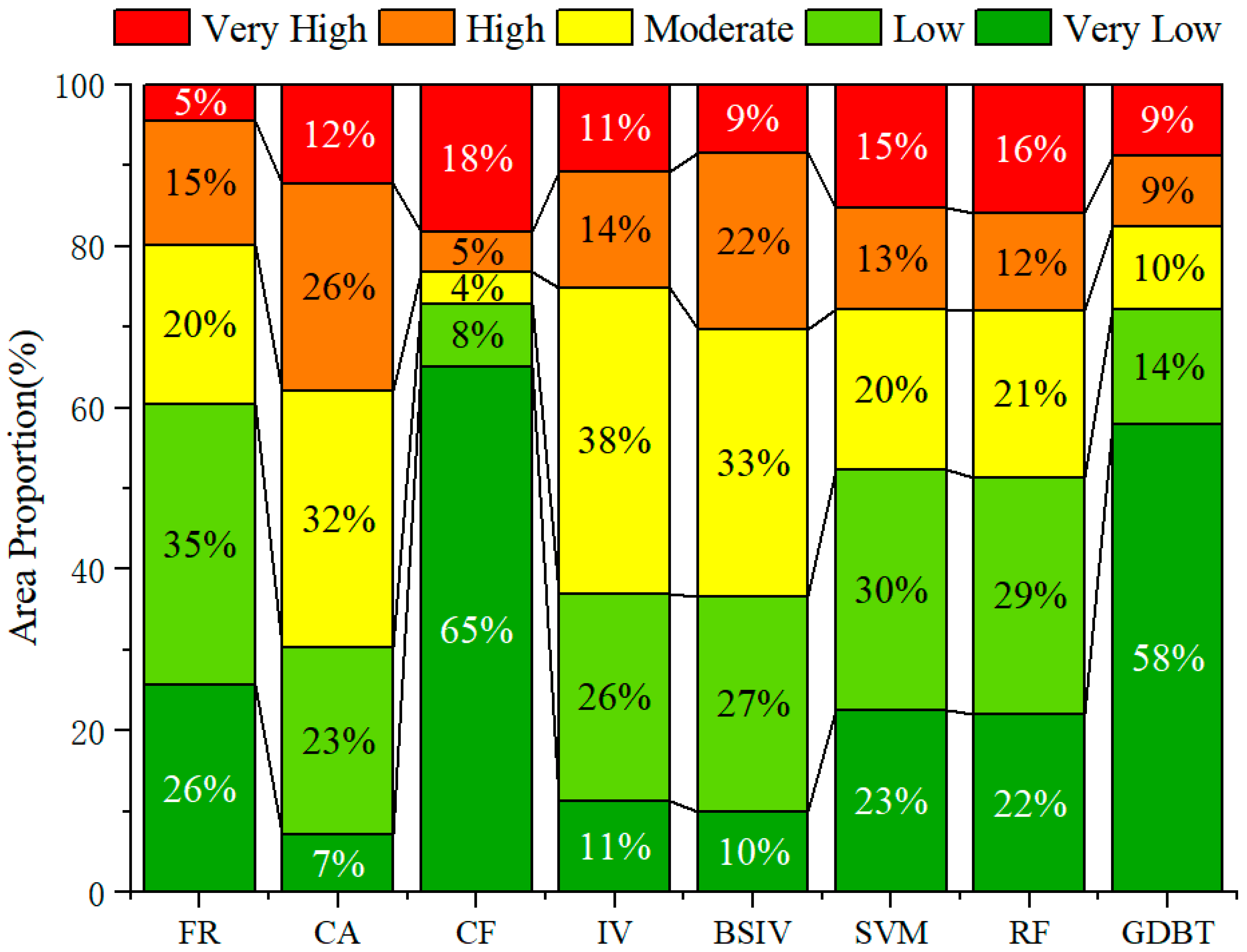
The landslide susceptibility evaluation results obtained from each model were statistically analyzed at all levels of the area (Figure 6). The area of very low susceptibility for the FR model was 236.39 km2, accounting for 25.66% of the total study region area. This area was mainly distributed around Changping, Yanshan, and Changling Townships. The low-susceptibility area was 320.97 km2, accounting for 34.84% of the total study area, and was primarily distributed around Shuaijia Village, Zhaojia Village, and Wanli Village. The medium susceptibility area was 181.31 km2, accounting for 19.68% of the total area, and was mainly distributed around Luojiaba, Zhongxing Village, and Hexikou. The high susceptibility area covers 141.41 km2, accounting for 15.35% of the study area’s total area. The extremely high susceptibility zone covers 41.84 km2, accounting for 4.54% of the total area, and is mainly located in Wanzhou city on the left bank of the Yangtze River. The very high susceptibility zone is primarily located near water systems and consists of Cambrian siltstone and sandstone, Silurian shale and sandstone, millstone, and Tertiary greywacke. These are loose and crumbly and prone to landslides. In the landslide susceptibility zoning of the CA model, the area of the very high susceptibility zone is 112.72 km2, accounting for 12.24% of the study area. It is mainly distributed on both sides of the Yangtze River in Wanzhou City. The area share of landslide susceptibility zones for models IV and BSIV is similar, with very high susceptibility zones covering 99.59 km2 and 73.53 km2, respectively. These zones are primarily located on both sides of the Dewuidu River and Dewuidu Town, accounting for 10% of the total area. The area’s share of very high susceptibility zones, obtained by evaluating the landslide susceptibility of model CF, is 168.08 km2, accounting for 18.24% of the total study area. The area and ratio of the very high susceptibility zones obtained from the SVM, RF, and GDBT models were 156.19 km2 (16.95%), 147.14 km2 (15.97%), and 80.93 km2 (8.87%), respectively.

4.3. Evaluation of Model Accuracy

4.3.1. The Statistical Table of Grids

Based on the results of the susceptibility evaluation in different models, the number of landslide grids under each susceptibility class, the proportion of landslides, the proportion of landslide grids in the total landslides, and the ratio of landslides for each class were counted. The detailed data are shown in Figure 7, where the proportion of landslides represents the number of landslide grids within each LS class, reflecting the proportion of landslides. Landslide ratio represents the ratio of the proportion of landslides under each LS class to the proportion of landslides across the entire area.
From Figure 7a,b, it can be seen that in the very low LS class, the number of landslide rasters in CF is the highest (the number reached 1350), which accounts for 0.20% of the number of rasters in this class. The number of several other models is low, accounting for less than 0.1% of the total number of rasters. In the low LS class, the number of individual models did not differ significantly, with the number distributed within the interval of 500–1000. The percentage of the CF model area was notably higher than the other values, at 1.24%. The pattern of the different models was similar in the moderate and high LS levels, with the highest number being FR, followed by IV, and the lowest being CF. The high susceptibility level had a relatively high proportion of FR at 8.47% and CA at 2.54%. In the very high susceptibility class, FR has the lowest number, followed by IV. The remaining six models have a slight difference in number. In terms of percentage, GDBT is ranked first with 20.26%, while the other models have a rate greater than 10%, except for BSIV. The model with the highest percentage of high and very high LS grades is GDBT, followed by FR. Several improved statistical analysis models have higher percentages than RF, SVM, and BSIV. The results show that although FR slightly underestimates the LS grades, the improved statistical analysis models have significantly improved sensitivity to LS and can obtain accurate evaluation results.
Figure 7c shows the proportion of the number of landslides in each LS class to the total number of landslides. The FR model has the highest proportion in the high susceptibility class, at 50.87%, followed by the very high class at 26.82%, the moderate class at 17.61%, and the low and very low classes, which account for less than 5%. The CA model has a high proportion of courses and a very high percentage compared to any other model, at 90.20%. The CF model has a relatively high proportion in both the very high and very low classes, with percentages of 79.61% and 5.16%, respectively. The IV and BSIV models have a total number in the high and very high courses of 89.55% and 75.16%. Grades are both high relative to the other models, with percentages of 79.61% and 5.16%, respectively. The IV and BSIV models have a total number of 89.55% and 75.29% in high and very high grades. The SVM, RF, and GDBT model slippage ratios exhibit some similarity, with the very high grades having the highest percentage, exceeding 60%, followed by the high grades, which have a rate in the 18–20% range.
The distribution patterns of landslide ratios and landslide proportions in Figure 7d are nearly identical, with some differences observed in the low and very high LS classes. At the very high levels, the ratios are listed in descending order: GDBT, FR, CA, IV, CF, SVM, RF, and BSIV. The higher ratio in the low LS level is CF, and FR has the highest ratio in the higher LS level. At the very high level, GDBT was ranked first with 7.95%, followed by FR, CA, IV, and CF in that order, all of which were higher than the remaining three models.

4.3.2. ROC Curves

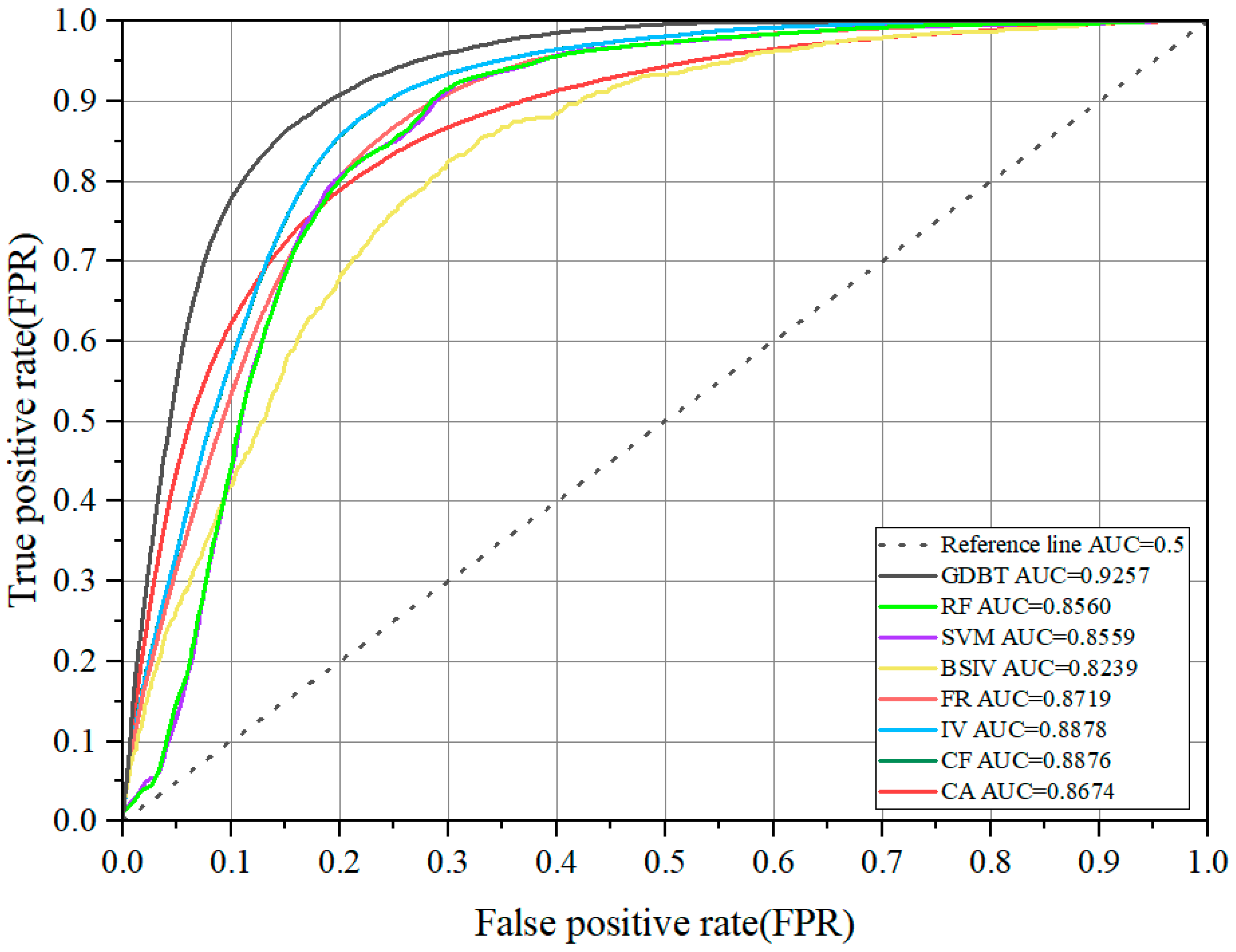
The computational results of several models (Figure 8) show that the GBDT model has the highest AUC value, followed by IV, CF, FR, CA, RF, SVM, and BSIV in descending order. The significantly higher AUC value of the continuous model compared to the traditional model and several machine learning models indicates a substantial improvement in performance metrics. Taking the IV model as an example, the AUC value is 0.8878, and the AUC value of BSIV is 0.8239, representing an increase of 0.0639. This value is also higher than those of machine learning models, such as RF and SVM, which are improved by 0.0318 and 0.0319, respectively. The improved statistical analysis method has demonstrated better results than the traditional method in evaluating landslide susceptibility.

4.3.3. Summary and Comparison of the LS Models

The performance and characteristics of all eight models are comprehensively summarized and compared in Table 2. The continuous models (FR, CA, CF, and IV) successfully bridge the gap between the interpretability of traditional statistical methods (BSIV) and the high predictive accuracy of machine learning models (SVM, RF, and GBDT).

5. Discussion

5.1. Quantitative Validation of Spatial Patterns

While the spatial concordance between high landslide susceptibility zones and known triggers like river proximity is visually evident (Figure 5), we performed a quantitative analysis to rigorously validate this observation. We calculated the average value of key triggering factors within the ‘Very High’ landslide susceptibility class for each model.
For instance, in the IV model, the average Distance to River within the ‘Very High’ landslide susceptibility zones is 407.13 m (Std. Dev. = 557.53 m). This is significantly less than the average distance across the entire study area (1996.90 m), confirming that areas extremely prone to landslides are overwhelmingly located in close proximity to the river. Similarly, the average Slope within these zones was 12.99 degrees, compared to the regional average of 16.27 degrees, and the average NDVI value was 0.29, indicating a specific vegetation profile associated with instability. This pattern was consistently observed across all statistical and machine learning models (e.g., RF model: Avg. Distance to River = 204.77 m; GBDT model: Avg. Distance to River = 279.34 m), providing robust quantitative evidence that LS accurately capture the geomorphological and environmental conditions that predispose the Wanzhou area to landslide.

5.2. Enhanced Interpretability Through Quantitative Continuous Models

Taking the IV model calculation as an example, the traditional statistical analysis method calculates the informativeness value by grading (or classifying) a limited number of factors. In contrast, this improved method enhances the differentiation between different graded values of factors by increasing the number of calculations. Theoretically, without setting the precision, the method can calculate a corresponding informativeness value for all values of the factor within the evaluation space. The method can be interpreted as a ‘sliding informativeness statistic’ for each factor value, using a uniform neighborhood window with overlap between the neighborhoods of individual factor values, and possible gaps in cases of low precision and small neighborhood windows. This not only increases the differentiation of the geohazard sensitivity of each factor but also reduces the subjectivity brought by the manual grading of the factors. The calculation process also becomes more controllable after making the ‘Bin Width’ the only control parameter that requires subjective input from the user. Additionally, the adoption of a unified parameter control will reduce manual input in evaluating geohazard susceptibility, enabling a rapid and automated assessment of geohazard susceptibility. For categorized influencing factors, such as geological lithology and land use type, the calculation is carried out according to the traditional method because it is not possible to transform the categorized information into continuous factor values.
From the results of calculating the informativeness values of different factors in the IV and BSIV models (Figure 9), we can determine the changes in landslide occurrence probability with factor values and reveal detailed, continuous changes. In the IV model, landslide susceptibility increases or decreases abruptly in response to changes in slope height, TST, and valley depth. However, the traditional method (BSIV) cannot accurately capture signals of sudden changes due to its limited number of gradations and inherent lag. Slope, Rainfall, NDVI, NDWI, Earthquake magnitude, and other factors exhibit more complex characteristics, with multiple mutation points and fluctuating values. Although the traditional method also displays a certain degree of volatility, the limited number of gradations means that the same level has the same value of information, which impacts the accuracy of the results.
Figure 9j shows the response curve of the NDVI factor. It indicates that when the NDVI value is between 0.4 and 0.6, the area with medium vegetation density may be sensitive to landslides. Therefore, the model does not simply rely on the presence of factors such as NDVI, but rather accurately captures the non-linear impact of their different numerical ranges on landslide probability. Removing a factor would result in the loss of this important pattern. More importantly, however, our method reveals the numerical conditions under which the factor is most critical.
The curve generated by the continuity model is able to clearly analyze the nonlinear relationship between various factors and landslide probability. It is evident that the precision of the model is contingent not solely on the incorporation of a specific factor, but also on the ability to accurately delineate the functional relationship between the factor and landslide occurrence. A group of factors with independent contributions and low redundancy was selected through rigorous Pearson correlation analysis (Figure 4). On this basis, the value of the continuous model lies in its ability to reveal the internal variation patterns of each factor with higher fidelity. Consequently, despite the absence of formal factor removal testing, analysis of continuous response curves suggests that our model exhibits considerable sensitivity to alterations in factor values, thereby enhancing the scientific rigor in the assessment of factor importance. The numerical-based sensitivity provides a more profound mechanism explanation than the simple existence-based sensitivity. Furthermore, it demonstrates that the model exhibits enhanced robustness and interpretability.
With the advancement of related technologies and the maturity of theories, various methods have been developed and applied to LS to improve prediction accuracy and reliability [15]. The GBDT model demonstrates a significantly higher predictive accuracy, as evidenced by the evaluation metrics (Table 2 and Figure 8). This finding underscores the GBDT model’s superiority over conventional quantitative continuous models in landslide susceptibility mapping within the Wanzhou region. Landslides are seldom caused by a single factor; rather, they result from complex interactions between multiple conditional and triggering factors [4]. The GBDT model, through its collection of decision trees, automatically detects and utilizes the complex interactions between variables, effectively identifying such complex nonlinear patterns and providing more stable and reliable estimation results [47].
However, machine learning, as a black box model, cannot visualize the spatial distribution of landslides under the conditions of each predisposing factor from the quantitative results [44]. The statistical analysis algorithm is advantageous in that it can systematically vary individual landslide-related factors in landslide susceptibility assessment in the same way as other methods and can approach or even exceed the accuracy of some machine learning algorithms when optimized using continuous models. Thus, the optimization approach can enhance the credibility, interpretability, and ease of operation of statistical analysis algorithms. It achieves a level of automation and objectivity closer to ML methods, removing the major subjectivity bottleneck of traditional statistical approaches. It does this without incurring the high computational and expertise costs associated with developing, tuning, and interpreting sophisticated ML models.
In conclusion, the trade-off is favorably resolved by our method: we sacrifice a small amount of pure predictive power (AUC) compared to the best-performing GBDT model, but we gain immensely in model transparency, physical interpretability.

5.3. Model Limitations and Future Research Directions

Despite the landslide susceptibility model constructed in this study demonstrating high accuracy in the Wanzhou, its performance is contingent on the unique local geological environment and landslide-inducing conditions (such as reservoir water level fluctuations and hilly terrain). It is therefore imperative to explore the model’s potential for application in areas with different landforms or triggering mechanisms. It is important to acknowledge that the application of this model to different regions may result in a substantial reduction in prediction accuracy. Future research could focus on transferring the above models and validating the effectiveness of the method framework in different geographical locations.
The accuracy of LS should not be the only priority; it is also crucial to identify the main conditions that lead to landslides, which can help to advance the process [48]. Several studies have focused on feature selection to identify suitable factors that can help reduce redundant information [49,50]. To further enhance susceptibility modelling, future studies should consider integrating multiple sources of data, such as time-series rainfall, remotely sensed change detection, and real-time monitoring data [51,52]. InSAR deformation monitoring data or geohazard monitoring station data could also be used to validate the dynamic accuracy of susceptibility zoning further [53].

6. Conclusions

This paper compares the performance of LS in Wanzhou based on continuous models using FR, CA, CF, and IV models, and compares the results with optimization algorithmic methods such as BSIV, SVM, RF, and GDBT. The following conclusions are drawn:
(1)
The susceptibility zoning shows that the extremely high-risk zones are concentrated along the main stream of the Yangtze River and the built-up areas of cities and towns, which is more consistent with the spatial distribution of historical landslides, and this distribution pattern confirms the synergistic mechanism of the reservoir level fluctuation and engineering activities.
(2)
The susceptibility maps generated by the continuous model are less patchy, and the spatial continuity is significantly improved. Compared with the traditional BSIV model, the AUC value is increased to 0.8878, which is close to the machine learning model accuracy.
(3)
The continuous model processing technique effectively solves the subjectivity problem of factor grading in the traditional statistical method. It achieves continuous quantification of the sensitivity of disaster-causing factors through the dynamic window sliding calculation, which can successfully capture the nonlinear response characteristics of factors such as slope and earthquake magnitude.

Author Contributions

Conceptualization, S.W.; Data curation, S.X., Y.S. and J.L.; Formal analysis, L.Z.; Funding acquisition, X.N. and M.Z.; Methodology, S.W.; Resources, L.Z.; Supervision, X.N.; Validation, S.W. and X.N.; Visualization, Y.S.; Writing—original draft, S.W. and S.X. All authors have read and agreed to the published version of the manuscript.

Funding

This research was funded by Geological Survey Project of China Geological Survey (Grant Nos. DD20230103, DD20243500, and DD20230495), Ministry of Natural Resources Provincial Cooperation Project (Grant No. 2023ZRBSHZ008), Anhui Public Welfare Geological Project of the Anhui Provincial Department of Natural Resources (Grant No. 2025-g-21).

Institutional Review Board Statement

Not applicable.

Informed Consent Statement

Not applicable.

Data Availability Statement

The data used in this study are not publicly available due to confidentiality and security restrictions regarding sensitive geological hazard information. Data may be available from the corresponding author upon reasonable request.

Conflicts of Interest

The authors declare no conflicts of interest.

References

  1. Kalantar, B.; Ueda, N.; Saeidi, V.; Ahmadi, K.; Halin, A.A.; Shabani, F. Landslide Susceptibility Mapping: Machine and ensemble learning based on remote sensing big data. Remote Sens. 2020, 12, 1737. [Google Scholar] [CrossRef]
  2. Karagianni, A.; Lazos, I.; Chatzipetros, A. Remote sensing techniques in disaster management: Amynteon Mine Landslides, Greece. In Intelligent Systems for Crisis Management; Lecture notes in geoinformation and cartography; Springer: Cham, Switzerland, 2019; pp. 209–235. [Google Scholar] [CrossRef]
  3. Liu, P.; Wei, Y.; Wang, Q.; Chen, Y.; Xie, J. Research on Post-Earthquake Landslide extraction algorithm based on improved U-Net model. Remote Sens. 2020, 12, 894. [Google Scholar] [CrossRef]
  4. Xu, S.; Song, Y.; Lu, P.; Mu, G.; Yang, K.; Wang, S. An optimized non-landslide sampling method for Landslide susceptibility evaluation using machine learning models. Nat. Hazards 2024, 121, 5873–5900. [Google Scholar] [CrossRef]
  5. Zhou, C.; Yin, K.; Cao, Y.; Ahmed, B.; Li, Y.; Catani, F.; Pourghasemi, H.R. Landslide susceptibility modeling applying machine learning methods: A case study from Longju in the Three Gorges Reservoir area, China. Comput. Geosci. 2017, 112, 23–37. [Google Scholar] [CrossRef]
  6. Frattini, P.; Crosta, G.; Carrara, A. Techniques for evaluating the performance of landslide susceptibility models. Eng. Geol. 2009, 111, 62–72. [Google Scholar] [CrossRef]
  7. Aleotti, P.; Chowdhury, R. Landslide hazard assessment: Summary review and new perspectives. Bull. Eng. Geol. Environ. 1999, 58, 21–44. [Google Scholar] [CrossRef]
  8. Casagli, N.; Intrieri, E.; Tofani, V.; Gigli, G.; Raspini, F. Landslide detection, monitoring and prediction with remote-sensing techniques. Nat. Rev. Earth Environ. 2023, 4, 51–64. [Google Scholar] [CrossRef]
  9. Xu, D.; Zhang, T.; Hei, L.; Wang, Y. Study on rainfall threshold of geological disasters based on effective rainfall model in Wenzhou City. East China Geol. 2025, 46, 252–267. (In Chinese) [Google Scholar] [CrossRef]
  10. Clerici, A.; Perego, S.; Tellini, C.; Vescovi, P. A GIS-based automated procedure for landslide susceptibility mapping by the Conditional Analysis method: The Baganza valley case study (Italian Northern Apennines). Environ. Geol. 2006, 50, 941–961. [Google Scholar] [CrossRef]
  11. Abeysiriwardana, H.D.; Gomes, P.I.A. Integrating vegetation indices and geo-environmental factors in GIS-based landslide-susceptibility mapping: Using logistic regression. J. Mt. Sci. 2022, 19, 477–492. [Google Scholar] [CrossRef]
  12. Gameiro, S.; Riffel, E.S.; De Oliveira, G.G.; Guasselli, L.A. Artificial neural networks applied to landslide susceptibility: The effect of sampling areas on model capacity for generalization and extrapolation. Appl. Geogr. 2021, 137, 102598. [Google Scholar] [CrossRef]
  13. Ikram, N.; Basharat, M.; Ali, A.; Usmani, N.A.; Gardezi, S.A.H.; Hussain, M.L.; Riaz, M.T. Comparison of landslide susceptibility models and their robustness analysis: A case study from the NW Himalayas, Pakistan. Geocarto Int. 2021, 37, 9204–9241. [Google Scholar] [CrossRef]
  14. Chang, L.; Xing, G.; Yin, H.; Fan, L.; Zhang, R.; Zhao, N.; Huang, F.; Ma, J. Landslide susceptibility evaluation and interpretability analysis of typical loess areas based on deep learning. Nat. Hazards Res. 2023, 3, 155–169. [Google Scholar] [CrossRef]
  15. Chang, Z.; Catani, F.; Huang, F.; Liu, G.; Meena, S.R.; Huang, J.; Zhou, C. Landslide susceptibility prediction using slope unit-based machine learning models considering the heterogeneity of conditioning factors. J. Rock Mech. Geotech. Eng. 2022, 15, 1127–1143. [Google Scholar] [CrossRef]
  16. Li, L.; Lan, H. Bivariate landslide susceptibility Analysis: Clarification, optimization, open software, and preliminary comparison. Remote Sens. 2023, 15, 1418. [Google Scholar] [CrossRef]
  17. Pourghasemi, H.R.; Yansari, Z.T.; Panagos, P.; Pradhan, B. Analysis and evaluation of landslide susceptibility: A review on articles published during 2005–2016 (periods of 2005–2012 and 2013–2016). Arab. J. Geosci. 2018, 11, 193. [Google Scholar] [CrossRef]
  18. Yin, K.; Zhu, L. Landslide hazard zonation and application of GIS. Earth Sci. Front. 2001, 8, 279–284. (In Chinese) [Google Scholar]
  19. Li, L.; Lan, H.; Guo, C.; Zhang, Y.; Li, Q.; Wu, Y. A modified frequency ratio method for landslide susceptibility assessment. Landslides 2016, 14, 727–741. [Google Scholar] [CrossRef]
  20. Van Westen, C. Application of Geographic Information Systems to Landslide Hazard Zonation. Ph.D. Thesis, Delft University of Technology, Delft, The Netherlands, 1993. Available online: http://repository.tudelft.nl/islandora/object/uuid%3Aa59d2eca-ab58-41e6-91c9-01e4e090cf81/datastream/OBJ/view (accessed on 5 May 2024).
  21. Dam, N.D.; Amiri, M.; Al-Ansari, N.; Prakash, I.; Van Le, H.; Nguyen, H.B.T.; Pham, B.T. Evaluation of Shannon Entropy and Weights of evidence models in landslide susceptibility mapping for the Pithoragarh district of Uttarakhand State, India. Adv. Civ. Eng. 2022, 2022, 6645007. [Google Scholar] [CrossRef]
  22. Zhou, C.; Gan, L.; Cao, Y.; Wang, Y.; Segoni, S.; Shi, X.; Motagh, M.; Singh, R.P. Landslide susceptibility assessment of the Wanzhou district: Merging landslide susceptibility modelling (LSM) with InSAR-derived ground deformation map. Int. J. Appl. Earth Obs. Geoinf. 2025, 136, 104365. [Google Scholar] [CrossRef]
  23. Song, Y.; Niu, R.; Xu, S.; Ye, R.; Peng, L.; Guo, T.; Li, S.; Chen, T. Landslide susceptibility mapping based on weighted gradient boosting decision tree in Wanzhou section of the Three Gorges Reservoir area (China). ISPRS Int. J. Geo-Inf. 2018, 8, 4. [Google Scholar] [CrossRef]
  24. Wang, J.; Xiao, L.; Zhang, J.; Zhu, Y. Deformation characteristics and failure mechanisms of a rainfall-induced complex landslide in Wanzhou County, Three Gorges Reservoir, China. Landslides 2019, 17, 419–431. [Google Scholar] [CrossRef]
  25. De Reu, J.; Bourgeois, J.; Bats, M.; Zwertvaegher, A.; Gelorini, V.; De Smedt, P.; Chu, W.; Antrop, M.; De Maeyer, P.; Finke, P.; et al. Application of the topographic position index to heterogeneous landscapes. Geomorphology 2012, 186, 39–49. [Google Scholar] [CrossRef]
  26. Mieza, M.S.; Cravero, W.R.; Kovac, F.D.; Bargiano, P.G. Delineation of site-specific management units for operational applications using the topographic position index in La Pampa, Argentina. Comput. Electron. Agric. 2016, 127, 158–167. [Google Scholar] [CrossRef]
  27. Couteron, P.; Barbier, N.; Gautier, D. Textural ordination based on Fourier Spectral decomposition: A method to analyze and compare landscape patterns. Landsc. Ecol. 2006, 21, 555–567. [Google Scholar] [CrossRef]
  28. Bugnicourt, P.; Guitet, S.; Santos, V.F.; Blanc, L.; Sotta, E.D.; Barbier, N.; Couteron, P. Using textural analysis for regional landform and landscape mapping, Eastern Guiana Shield. Geomorphology 2018, 317, 23–44. [Google Scholar] [CrossRef]
  29. Berti, M.; Corsini, A.; Daehne, A. Comparative analysis of surface roughness algorithms for the identification of active landslides. Geomorphology 2012, 182, 1–18. [Google Scholar] [CrossRef]
  30. Mhiret, D.A.; Dagnew, D.C.; Assefa, T.T.; Tilahun, S.A.; Zaitchik, B.F.; Steenhuis, T.S. Erosion hotspot identification in the sub-humid Ethiopian highlands. Ecohydrol. Hydrobiol. 2018, 19, 146–154. [Google Scholar] [CrossRef]
  31. Mohseni, N.; Salar, Y.S. Terrain indices control the quality of soil total carbon stock within water erosion-prone environments. Ecohydrol. Hydrobiol. 2020, 21, 46–54. [Google Scholar] [CrossRef]
  32. Li, D.; Huang, F.; Yan, L.; Cao, Z.; Chen, J.; Ye, Z. Landslide Susceptibility Prediction Using Particle-Swarm-Optimized Multilayer Perceptron: Comparisons with Multilayer-Perceptron-Only, BP Neural Network, and Information Value Models. Appl. Sci. 2019, 9, 3664. [Google Scholar] [CrossRef]
  33. Lan, H.; Zhou, C.; Wang, L.; Zhang, H.; Li, R. Landslide hazard spatial analysis and prediction using GIS in the Xiaojiang watershed, Yunnan, China. Eng. Geol. 2004, 76, 109–128. [Google Scholar] [CrossRef]
  34. Shortliffe, E.H.; Buchanan, B.G. A model of inexact reasoning in medicine. Math. Biosci. 1975, 23, 351–379. [Google Scholar] [CrossRef]
  35. Heckerman, D. Probabilistic Interpretations for Mycin’s Certainty Factors*. In Machine Intelligence and Pattern Recognition; *This work was supported in part by the Josiah Macy, Jr. Foundation, the Henry J. Kaiser Family Foundation, and the Ford Aerospace Corporation. Computing facilities were provided by the SUMEX-AIM resource under NIH grant RR-00785; Elsevier B.V.: Amsterdam, The Netherlands, 1986; pp. 167–196. [Google Scholar] [CrossRef]
  36. Ross, T.J. Fuzzy Logic with Engineering Applications. 2010. Available online: https://onlinelibrary.wiley.com/doi/book/10.1002/9781119994374 (accessed on 1 March 2025).
  37. Kanungo, D.; Arora, M.; Sarkar, S.; Gupta, R. A comparative study of conventional, ANN black box, fuzzy and combined neural and fuzzy weighting procedures for landslide susceptibility zonation in Darjeeling Himalayas. Eng. Geol. 2006, 85, 347–366. [Google Scholar] [CrossRef]
  38. Zhou, W.; Fang, J. Assessment of landslide susceptibility based on information quantity model and data normalization. J. Geo-Inf. Sci. 2018, 20, 674–683. (In Chinese) [Google Scholar] [CrossRef]
  39. Cortes, C.; Vapnik, V. Support-vector networks. Mach. Learn. 1995, 20, 273–297. [Google Scholar] [CrossRef]
  40. Pandey, V.K.; Pourghasemi, H.R.; Sharma, M.C. Landslide susceptibility mapping using maximum entropy and support vector machine models along the highway corridor, Garhwal Himalaya. Geocarto Int. 2018, 35, 168–187. [Google Scholar] [CrossRef]
  41. Han, Z.; Fang, Z.; Li, Y.; Fu, B. A novel Dynahead-Yolo neural network for the detection of landslides with variable proportions using remote sensing images. Front. Earth Sci. 2023, 10, 1077153. [Google Scholar] [CrossRef]
  42. Hong, H.; Miao, Y.; Liu, J.; Zhu, A. Exploring the effects of the design and quantity of absence data on the performance of random forest-based landslide susceptibility mapping. CATENA 2019, 176, 45–64. [Google Scholar] [CrossRef]
  43. Merghadi, A.; Yunus, A.P.; Dou, J.; Whiteley, J.; ThaiPham, B.; Bui, D.T.; Avtar, R.; Abderrahmane, B. Machine learning methods for landslide susceptibility studies: A comparative overview of algorithm performance. Earth-Sci. Rev. 2020, 207, 103225. [Google Scholar] [CrossRef]
  44. Zhang, Y.; Lan, H.; Li, L.; Wu, Y.; Chen, J.; Tian, N. Optimizing the frequency ratio method for landslide susceptibility assessment: A case study of the Caiyuan Basin in the southeast mountainous area of China. J. Mt. Sci. 2020, 17, 340–357. [Google Scholar] [CrossRef]
  45. Pourghasemi, H.R.; Jirandeh, A.G.; Pradhan, B.; Xu, C.; Gokceoglu, C. Landslide susceptibility mapping using support vector machine and GIS at the Golestan Province, Iran. J. Earth Syst. Sci. 2013, 122, 349–369. [Google Scholar] [CrossRef]
  46. Bui, D.T.; Pradhan, B.; Lofman, O.; Revhaug, I.; Dick, Ø.B. Regional prediction of landslide hazard using probability analysis of intense rainfall in the Hoa Binh province, Vietnam. Nat. Hazards 2012, 66, 707–730. [Google Scholar] [CrossRef]
  47. Yang, K.; Niu, R.; Song, Y.; Dong, J.; Zhang, H.; Chen, J. Dynamic Hazard Assessment of Rainfall-Induced Landslides Using Gradient Boosting Decision Tree with Google Earth Engine in Three Gorges Reservoir Area, China. Water 2024, 16, 1638. [Google Scholar] [CrossRef]
  48. Murillo-García, F.G.; Steger, S.; Alcántara-Ayala, I. Landslide susceptibility: A statistically-based assessment on a depositional pyroclastic ramp. J. Mt. Sci. 2019, 16, 561–580. [Google Scholar] [CrossRef]
  49. Sun, L.; Zhang, H.; Qiu, C.; Yang, Z.; Zhang, C.; Zhang, B.; Zhang, T. Temporal variability of influence factors weights and rainfall thresholds of geological hazards in Ningbo City. East China Geol. 2024, 45, 218–227. (In Chinese) [Google Scholar] [CrossRef]
  50. Bukhari, M.H.; Da Silva, P.F.; Pilz, J.; Istanbulluoglu, E.; Görüm, T.; Lee, J.; Karamehic-Muratovic, A.; Urmi, T.; Soltani, A.; Wilopo, W.; et al. Community perceptions of landslide risk and susceptibility: A multi-country study. Landslides 2023, 20, 1321–1334. [Google Scholar] [CrossRef]
  51. Liu, L.; Wang, P.; Su, L.; Li, F. Landslide data sample augmentation and landslide susceptibility analysis in Nyingchi City based on the MCMC model. Sci. Rep. 2025, 15, 25624. [Google Scholar] [CrossRef]
  52. Arabameri, A.; Pradhan, B.; Rezaei, K.; Lee, C. Assessment of landslide susceptibility using Statistical- and Artificial Intelligence-Based FR–RF integrated model and multiresolution DEMs. Remote Sens. 2019, 11, 999. [Google Scholar] [CrossRef]
  53. Wang, P.; Deng, H.; Li, Y.; Pan, Z.; Peng, T. Enhancing landslide susceptibility modelling through predicted InSAR deformation rates. Environ. Earth Sci. 2025, 84, 347. [Google Scholar] [CrossRef]
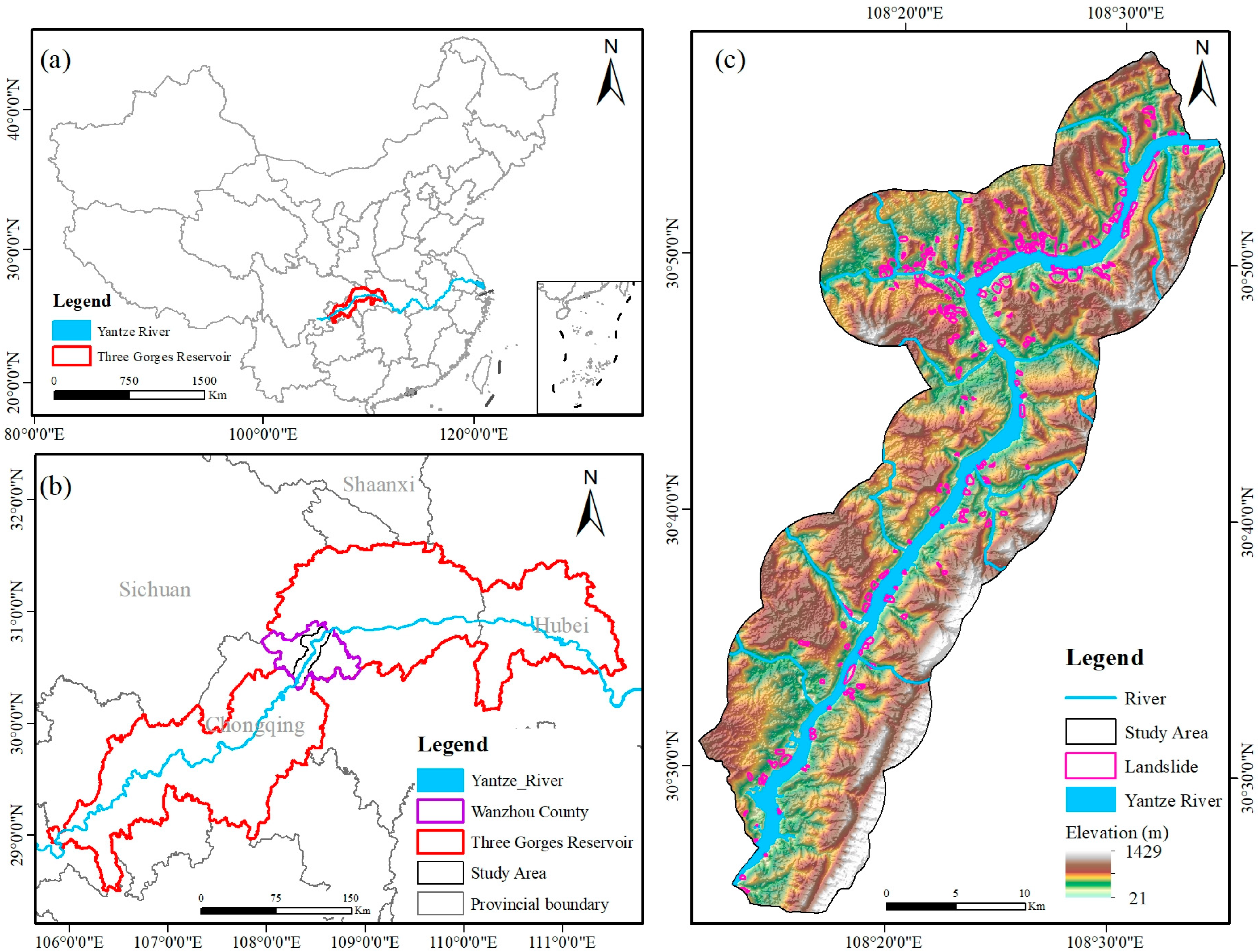
Figure 1. Location of the study area: (a) Location of the Three Gorges Reservoir Area in China; (b) Location of the study area in the Three Gorges Reservoir Area; (c) Location of the study area and distribution of landslides.
Geohazards 06 00048 g001
Figure 2. Landslide-causing factors. (ar), respectively, represent Engineering rock group, elevation, slope, slope height, aspect, profile curvature, plain curvature, TST, TRI, TPI, TWI, valley depth, distance to river, rainfall, NDVI, NDWI, magnitude of earthquake, and land use.
Geohazards 06 00048 g002
Figure 3. Framework of this study.
Geohazards 06 00048 g003
Figure 4. Pearson’s correlation of 18 landslide-causing factors. F1–F18 represents the Engineering rock group, elevation, slope, slope height, aspect, profile curvature, plain curvature, TST, TRI, TPI, TWI, valley depth, distance to river, rainfall, NDVI, NDWI, magnitude of earthquake, and land use.
Geohazards 06 00048 g004
Figure 5. LS mapping results using different machine models. (ah) represent the LS zoning results based on FR, CA, CF, IV, BSIV, SVM, RF, and GDBT models, respectively.
Geohazards 06 00048 g005
Figure 6. Percentage of area in different LS classes.
Geohazards 06 00048 g006
Figure 7. Percentage of area in different LS classes. (a) The number of landslide grids under each LS class; (b) The proportion of landslides; (c) The proportion of landslide grids in the total landslides; (d) The ratio of landslides for each LS class.
Geohazards 06 00048 g007
Figure 8. ROC curves for different models.
Geohazards 06 00048 g008
Figure 9. Variations in favorability value with factor values. (a) Slope. (b) Magnitude of earthquake. (c) Slope height. (d) Aspect. (e) TST. (f) TPI. (g)Valley depth. (h) Distance to river. (i) Rainfall. (j) NDVI. (k) NDWI.
Geohazards 06 00048 g009
Table 1. Sources of factors and data extraction methods.
CategoryFactorData SourceData Extraction MethodsFactor ID
GeologicalEngineered Rock GroupNational Geological Data MuseumFrom the 1:50,000 geological map, the factor is classified into four categories based on its engineering mechanical properties: Carbonate Formation (I), Thick Hard Sandstone Formation (II), Soft and Hard Interbedded Sandstone and Mudstone Formation (III), and Thinly Layered Weak Claystone Formation (IV), as shown in Figure 2a.F1
TopographicalElevationGeospatial Data Cloud PlatformDEM data, Figure 2bF2
SlopeUse the slope module in ArcGIS, Figure 2cF3
Slope heightUse the focal statistics module in ArcGIS, Figure 2dF4
AspectUse the aspect module in ArcGIS, Figure 2eF5
Profile curvatureUse the curvature module in ArcGIS, Figure 2fF6
Plain curvatureUse the curvature module in ArcGIS, Figure 2gF7
TSTUse raster analysis tools in QGIS, Figure 2h [25,26]F8
TRITRI = 1/Cos(‘Slope’ × 3.14/180), Figure 2i [27]F9
TPIUse the map algebra tool in ArcGIS, Figure 2j [28,29]F10
HydrologicalTWIGeospatial Data Cloud PlatformUse hydrology and map algebra tools in ArcGIS, Figure 2k [30,31]F11
Valley depthUse the Valley Depth module in SAGA, Figure 2lF12
Distance to riverNational Geological Data MuseumUse the Euclidean distance module in ArcGIS, Figure 2mF13
EnvironmentalRainfallChina Meteorological Data NetworkUse the Inverse Distance Weighting (IDW) module in ArcGIS, based on annual precipitation at meteorological stations from 2010 to 2020, Figure 2nF14
NDVILandsat-8 imagery, Geographic Information Cloud PlatformUse the NDVI module in ENVI, based on Landsat-8 imagery (8 December 2013, row/column number 152/39), Figure 2oF15
NDWIUse the Band Math in ENVI, based on Landsat-8 imagery (8 December 2013, path/row 152/39), Figure 2pF16
Magnitude of earthquakeChina Earthquake Networks CentreUse the Kriging Interpolation module in ArcGIS, based on historical earthquakes from 1970 to 2020, Figure 2qF17
Land useEsri Land CoverFive categories: water, built area, forest, agriculture, grassland, Figure 2rF18
Table 2. Summary and comparison of the LS models.
ModelKey AdvantageKey LimitationAUC ValueLandslides over High LS/
Total Number of Landslides
IVHigh interpretability, captures continuous factor responses, and reduces subjectivity [32]Slightly lower AUC than top ML models0.88780.8954
FRSimple principle, easy to implement and understand [20]May slightly underestimate susceptibility0.87190.7769
CFHandles uncertainty in data, combines evidence effectively [33]Calculation is more complex than FR/IV0.88760.8761
CAMeasures similarity based on vector anglesInterpretation can be less intuitive than probability-based methods [36]0.86740.9020
BSIVStandardizes information values across factors [4]Subjective grading misses continuous variations0.82390.7529
SVMEffective in high-dimensional spaces, good for non-linear problems [40]“Black-box” nature, poor interpretability, sensitive to parameters0.83990.8639
RFHigh accuracy, handles non-linearity well, reduces overfitting [41]“Black-box” nature, poor interpretability0.85690.8693
GBDTHighest accuracy, often superior performance [43]“Black-box” nature, most complex, computationally intensive0.92570.8771
Disclaimer/Publisher’s Note: The statements, opinions and data contained in all publications are solely those of the individual author(s) and contributor(s) and not of MDPI and/or the editor(s). MDPI and/or the editor(s) disclaim responsibility for any injury to people or property resulting from any ideas, methods, instructions or products referred to in the content.