Abstract
The prevalence of unforeseen floods has heightened the need for more accurate flood simulation and forecasting models. Even though forecast stations are expanding across the United States, the coverage is usually limited to major rivers and urban areas. Most rural and sub-urban areas, including recreational areas such as the Window Cliffs State Natural Area, do not have such forecast stations and as such, are prone to the dire effects of unforeseen flooding. In this study, four machine learning model architectures were developed based on the long short-term memory, random forest, and support vector regression techniques to forecast water depths at the Window Cliffs State Natural Area, located within the Cane Creek watershed in Putnam County, Tennessee. Historic upstream and downstream water levels and absolute pressure were used to forecast the future water levels downstream of the Cane Creek watershed. The models were tested with lead times of 3, 4, 5, and 6 h, revealing that the model performances reduced with an increase in lead time. Even though the models yielded low errors of 0.063–0.368 ft MAE, there was an apparent delay in predicting the peak water depths. However, including rainfall data in the forecast showed a promising improvement in the models’ performance. Tests conducted on the Cumberland River in Tennessee showed a promising improvement in model performance when trained with larger data.
1. Introduction
Flooding is a devastating natural disaster across the globe with increasing frequency and impacts in recent decades [1,2]. In the United States of America (U.S.), floods constitute the most prevalent natural disaster, costing about USD 4.6 billion and claiming about 18 lives per event on average. From 2010 to 2020, a total of 212 lives were lost to major flooding events in the U.S. [3]. The effects of floods are even worse when evacuations are not performed in time [4]. Flash floods usually occur without conceivable warning, and as such, may lead to injury, loss of lives, and property damage. The degree of flood hazards has heightened the need for more accurate flood prediction and simulation models.
Floods can be forecasted by simulating flood events with either physically based models or data-driven models. Physically based models are based on the principles of physics governing streamflow. Physically based models usually require different types of hydro-geomorphological monitoring datasets, intensive computational demands, and in-depth knowledge and expertise regarding the hydrological parameters that impede the short-term prediction capabilities of physically based models [5]. Also, physically based models do not account for uncertainties such as underground flow in karst landforms [6]. The data-driven models, on the other hand, find a logical relationship between the input and output parameters [7,8] involved in the simulation. This includes the use of machine learning to forecast water levels [9].
The use of machine learning in flood forecasting can be classified under data-driven models. In a broad context, machine learning can be defined as the use of ‘‘a computer program to learn from experience E with respect to some task T and a performance measure P, if its performance at tasks in T, as measured by P, improves with experience E” [10] (p. 2). In the context of flood forecasting, the experience can be a set of input data, , where Y and X represent the continuous, observed water levels and their corresponding feature matrix of N observations. The task of a machine learning model is to find an unknown function which can be used to predict water levels, , as close to the actual observations as possible based on a particular performance measure [9].
There are several factors that need to be taken into consideration to generate accurate flood forecasts using conventional physically based models. Due to the difficulty and high level of skill involved in the conventional methods, there has been a gradual introduction and shift towards the use of machine learning techniques for flood forecasting [11]. Machine learning techniques do not require users to know the exact underlying processes behind the flood models. Some of the recent advancements in the use of machine learning for flood forecasting include techniques such as linear regression, gradient boosting, support vector machine, and ensemble learning [11]. Ref. [9] tested the use of the least absolute shrinkage and selection operator (LASSO), random forest, and support vector regression (SVR) machine learning approaches in forecasting 5-lead-day water levels downstream along the Mekong River, Vietnam. In their experiments, Ref. [9] evaluated their models using the mean absolute error (MAE), root mean squared error, and coefficient of the efficiency metrics. Based on these evaluation metrics, the SVR performed best in predicting the 5-lead-day forecast water levels. Another form of machine learning technique that has been used in flood forecasting is the long short-term memory (LSTM) neural network which is the core architecture behind the stage forecasting in Google’s end-to-end operational flood warning system that has been applied in India and Bangladesh [12]. This machine learning model was able to predict floods during the monsoon season in 2021 and warn the residents and the necessary authorities. This is an example of how important the use of machine-learning-based models can be in saving lives. The use of LSTM-based models has been proven to estimate extreme events even when events of similar magnitude are not included in the training dataset [13].
Flood forecasting in the U.S. has evolved over the years. Currently, the National Weather Service (NWS) has 13 river forecasting centers (RFCs) which are in charge of all the hydraulic and hydrologic modeling involved in public streamflow forecasts [14]. Even though the RFCs work independently, they all use similar operational models that are customized to suit local needs. A typical example is the advanced hydrologic prediction service (AHPS; [15]) which is implemented at the RFCs in predicting river levels with longer lead times. The coverage of the AHPS is expanding across the U.S. at an accelerated rate with about 3000 forecast stations in the U.S. as of 2021.
Despite the fast expansion of the AHPS, many small streams and areas do not have forecast stations. As of November 2021, there were 73 forecast points in the state of Tennessee that mostly covered the major rivers and urban areas. Out of the 95 counties in the state of Tennessee, 50 of them, including Putnam County, do not have any river forecast station [16]. Among the seven neighboring counties of Putnam County, only Smith County has a forecasting point (Figure 1). However, flooding remains an issue in several rural and suburban areas where there is no river forecast point.
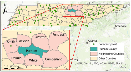
Figure 1.
National Weather Service Forecast Points in the state of Tennessee. There is one forecasting station in Putnam County and its neighboring counties combined [16].
Floods in some state parks in and around Putnam County have been in the news recently. For instance, in August 2017, a flash flood claimed the lives of two women, including a 73-year-old and a volunteer rescue worker, at the Cummins Falls State Park, TN. The same event left 40 people stranded at the Blackburn Fork State Scenic River, upstream of Cummins Falls [17]. Two years later, another flash flood led to the loss of a two-year-old boy at the Cummins Falls State Natural area. Even though the office of the National Weather Service had communicated the possibility of rain to the park managers, it was not easy to associate the anticipated amount of rainfall with a fatal flood event. Ref. [18] reported that, on a regular day, evacuation begins when the park’s staff observes a certain threshold water level. There is, therefore, the need to expand the water level forecast to such areas that are prone to flash flooding to help prevent any future loss of lives.
The objective of this study is to develop a water-level forecasting system for Window Cliffs State Natural Area (Window Cliffs) based on which flood warnings can be issued ahead of time. When there is an imminent flood event, the system will generate forecasts with an ample lead time to allow for the safe evacuation or closure of the park. The flood forecast is based on the predicted water level downstream, at Window Cliffs’ first creek crossing (C1). In this study, machine learning techniques were used to develop the flood forecasting system.
Window Cliffs was selected as the study area because of the accessible water monitoring devices and gauge stations within and around the park. This study is a build-up on previous work performed by [19] to develop an early flood warning system for Window Cliffs that could predict the historical water level downstream of the Cane Creek stream, given the historical upstream flow parameters and precipitation data.
This study developed a forecasting system that can predict floods using basic climatic and hydrologic data without the need for complex hydraulic and hydrologic modeling methods that often require a lot of data on the physical characteristics of the watershed. This approach is easily applicable to other watersheds that have limited data and can capture complex relationships that cannot be easily represented in physical models. Once developed, they can adapt to changing conditions and learn from new data, thereby improving their accuracy over time compared to traditional forecasting systems.
2. Materials and Methods
2.1. Study Area
Window Cliffs is a 1.11 km2 (275-acre) recreational area located in the southwestern part of Putnam County, located in the state of Tennessee in the U.S. About 3.9 km (2.4 mi) stream length of Cane Creek flows through Window Cliffs. The recreational area also features a 2.7-mile trail that crosses Cane Creek 10 times [20]. Window Cliffs lies at the downstream section of the entire Cane Creek watershed (HUC-051301080703; Figure 2). The Phelps Branch is Cane Creek’s major tributary. The entire Cane Creek watershed is located in the Eastern Highland Rim in Tennessee. The watershed has a highly developed karst geology [20,21]. The Cane Creek watershed has a total area of 62.35 km2 (15,408.16 acres) oriented from northeast to southwest (Figure 2).
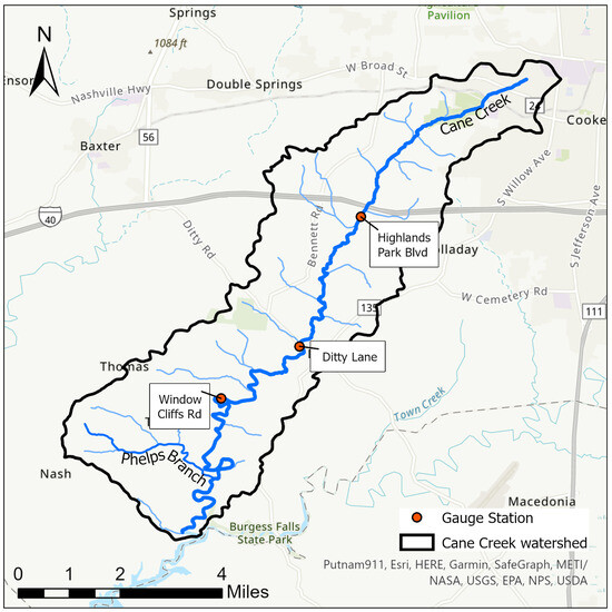
Figure 2.
Cane Creek watershed.
Although rainfall is a primary driver of runoff processes, rainfall may not directly translate into runoff owing to the porous and karst landform in the study area. Rainfall seeps underground and reduces its impact on surface runoff and the downstream water level. The karst landform, in other cases, also contributes the unaccounted underground flow to the streamflow of Cane Creek.
Over the years, there have been several flash flood events at the Window Cliffs State Natural Area. Currently, the park’s management relies on three water monitoring stations and weather forecasts to determine whether or not to close the park when imminent flooding is probable.
2.2. Data Collection and Preparation
Machine learning requires a sufficient amount of related input and output data. In similar studies, Ref. [19] used the time series of “upstream water levels, precipitation and antecedent dry period” as input datasets to forecast water levels [19] (p. 20). Additional data that have been used in previous studies include temperature, characterized convective weather systems, and wind direction data [22]. For this study, the data were collected from measuring devices installed by Tennessee Tech University (TTU) and the Tennessee Department of Environment and Conservation (TDEC) along the Cane Creek at Window Cliffs, Window Cliffs road, Ditty Road, and Highland Park Boulevard (Figure 2).
A six-character alphanumeric nomenclature was adopted to allow one to easily make reference to the available data. The first two characters in the nomenclature represent the location of the measuring device, whilst the third and fourth characters signify the type of data and the last two characters denote the owner of the data logger (Table 1). For example, rainfall data collected from Highland Park Boulevard by a TDEC measuring device is referred to as HP-RF-TD.

Table 1.
Available sources of data within the Cane Creek watershed.
There were 20 available forms of data from all five data locations. There were three TTU loggers at Cane Creek crossing 1, Cane Creek crossing 10, and Window Cliffs Road that measured absolute pressure, barometric pressure, differential pressure, temperature, and water depth. There was another TTU measuring device located at Ditty Road that recorded water surface elevation. TDEC had a measuring device at Highland Park Boulevard that measured rainfall, a measuring device at Window Cliffs Road that measured water level, and another device at Ditty Road that measured both rainfall and water level.
Apart from data from Cane Creek crossing 10, all other available data spanned across a common, overlapping time window between 6 November 2021, 12:00 and 5 January 2022, 10:00. Consistently continuous data during this time window were not available for Cane Creek crossing 10 (see Figure A1 in Appendix A). Therefore, data from Cane Creek crossing 10 were excluded from this study, leaving only 15 data forms to work with. Also, during the overlapping period, there were brief rainfall events recorded at Highland Park Boulevard that do not provide a time series long enough to for the overlapping period. The time interval for all the available data was resampled to a 1 h time interval. In this study, a 1 h time interval is synonymously referred to as a single time step.
Apart from the small amount of data being due to the short availability windows, the distribution of the available data had a lot of outliers. The outliers can introduce noise in the models and affect performance. Data from the downstream location at Creek Crossing 1 (C1-WD-TT), for example, had some extreme events that constituted the outliers. A distribution of the normalized data from the input features of the models can be seen in Figure A2 of Appendix B.
2.2.1. Data Correction and Rescaling
Water depth data at C1 (C1-WD-TT) had some negative values which could have been the result of an erroneous reference water level during the deployment and configuration of the measuring device. To correct the negative water depth values in C1-WD-TT, a positive constant with a magnitude equivalent to the minimum recorded water depth in C1-WD-TT was added to all the values in C1-WD-TT. This correction assumes that the minimum recorded water depth corresponds to a dry condition at the location of the measuring device. Therefore, all values in C1-WD-TT were adjusted upwards with a constant value of 0.255 m (0.839 ft) (Figure 3).
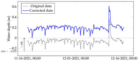
Figure 3.
Correction of water depth data at Cane Creek crossing 1. The original values in C1-WD-TT were adjusted upwards with a constant value of 0.255 m (0.839 ft). Data shown in this figure are from 16 November 2021 to 15 December 2021.
The input data were rescaled for efficient training during the model development phase. All the input data were normalized linearly between 0 and 1 using Equation (1):
where refers to the minimum value in the normalized domain, refers to the maximum value in the normalized domain, is the minimum value of the raw input data, is the maximum value of the raw input data, and refers to the ith value in the raw input data before normalization. The values fall between the range of and which were set to 0 and 1, respectively.
2.2.2. Feature Selection
The feature selection involved a series of tests to determine the input features with the most influence on the output of the model. The important input features were selected using the correlation analyses between a future downstream water level at a lead time of 6 h and input data from time steps to in history.
The data involved in this study can be classified under predictor and criterion variables. The predictor variables are used to predict the criterion variable. The criterion variable in this study is the water level at C1 at a future time step of either , , , or while the predictor variables include all other variables from time to in history. We calculated the Spearman’s rank correlation coefficient () between the future time step and the predictor variables to provide insight into which predictor variables were strong factors in predicting the criterion variable. Values of range from to where a value of indicates a perfect negative association, indicates a perfect association, and 0 means no association between two ranked variables. For a strong correlation, is closer to 1 while values closer to 0 represent a weak correlation. The Spearman’s rank correlation analysis was the initial step in eliminating weak data from the prediction problem.
Some of the predictor variables may be related to each other because some are derived from others. The proximity of measuring devices can also result in a strong correlation between the predictor variables. We conducted a cross-correlation to determine any multicollinearity between two or more of the shortlisted variables. This served as a secondary procedure to further reduce the size of predictor variables involved in forecasting the water level at C1.
2.2.3. Training, Testing, and Inference Data Split
The available dataset was split into training, testing, and inference sets. The training and testing sets comprised data from 6 November 2021, 12:00 to 31 December 2021, 23:00 while the inference set spanned from 1 January 2022, 00:00 to 5 January 2022, 10:00. After generating input–output pairs for training and testing, the input–output pairs were shuffled and split into a training set and a testing set ratio of 70:30, respectively. The inference set, on the other hand, was not shuffled.
The training and testing datasets were shuffled to generate an unbiased distribution and to capture a variety of event types (high- and low-water depths at C1) among the training and testing sets. The training set was used to train the models while the testing set was used to evaluate the performance of the trained models. The purpose of the inference set was to assess the models’ performances in generating outputs for a continuous, unshuffled dataset.
2.3. Machine Learning Model Development
The machine learning development involved the selection of suitable machine learning architectures, training, and model enhancement. All the candidate architectures were developed in parallel to assess their performances in the end. The models were developed in a Python 3 environment mainly by using TensorFlow [23] and Scikit-learn [24] packages.
The objective of the machine learning model is to find a function that receives a time-sequence of input features to predict the expected water level at a downstream location, C1, at a future time step. The function can be expressed as:
where refers to the predicted water level C1 at time step , l refers to the number of lead time steps, and referred to a sequence of input data from the present time, , to n timesteps in history. In this study, we assessed the lead time steps of 3, 4, 5, and 6 h for each of the candidate models.
2.3.1. Model Architecture Selection
Two variations of long short-term memory (LSTM; [25]), the SVR [26], and the random forest regression (RFR; [27]) models were assessed as candidates for the flood forecasting system. LSTM, a form of a recurrent neural network, is efficient in sequence problems while the SVR and RF models were also used in a similar study that forecast downstream water levels [9]. Details of the candidate architectures assessed in this study are outlined in this section.
2.3.2. LSTM Model 1
The LSTM Model 1 (LSTM 1) consists of two main components: an LSTM cell and at least one dense layer. The LSTM cell is a recurrent unit that has a memory component with the ability to forget, retain, and pass on information from previous steps along a sequence. The memory of the LSTM cell contains the cell state that holds the information to be passed on from one step in the sequence to another. The state of the memory is controlled by a set of functions that are called gates. There are three main gates in a standard LSTM cell, namely the forget gate, update gate, and output gate. The forget gate determines what information needs to be discarded from the memory while the update gate controls the information that needs to be added to the memory’s cell state. Based on the cell state at a particular step, the output gate generates the output of the LSTM cell.
In summary, an LSTM cell receives a cell state and an output from the previous step in the sequence and then combines it with input data to generate a cell state and an output to be passed on to the next step in the sequence. The output is then passed on to at least one densely connected neural network layer (dense layer) with a linear activation. The output of the dense layers is the forecast water level at C1.
Figure 4 is a schematic of the LSTM Model 1 that receives a sequence of input data to generate an output water level prediction . The LSTM Model 1 was constructed using the Keras module in TensorFlow.
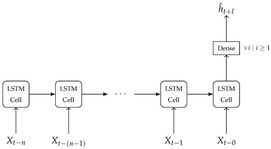
Figure 4.
Schematic of the LSTM Model 1. The recurrent LSTM cells receive a set of inputs to generate an output which is then passed onto at least one dense layer to generate a final output.
2.3.3. LSTM Model 2
The LSTM Model 2 (LSTM 2) is made up of an encoder component and a decoder component. The encoder component has the same structure as the LSTM Model 1 (Figure 4). The output of the encoder section is passed onto the decoder section. The decoder component is a sequence of LSTM cells preceding at least one dense layer. We have named the LSTM cells in the decoder component as decoder cells to distinguish them from the LSTM cells in the encoder component. Each decoder cell uses the previous time step’s water depth at the target location and information from either the encoder component or a preceding decoder cell to generate the water depth at the next time step. This process is recursively repeated until the final water depth is generated.
Figure 5 is a schematic of the LSTM Model 2 that receives a sequence of input data to generate a final output water level prediction . Like the LSTM Model 1, the LSTM Model 2 was constructed using the Keras module in TensorFlow.
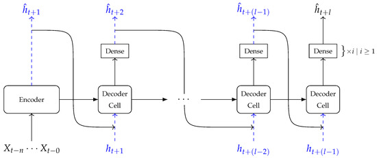
Figure 5.
Schematic of LSTM Model 2.
2.3.4. SVR Model
SVR is a representation of support-vector networks which was originally developed by [28] for two-group classification problems. The objective of the SVR model is to find a function that can approximate an unknown function within a specified error margin. x refers to an input vector of d elements where d is the dimensionality of the input space. The dimensionality of the input vector for the flood forecasting model is equivalent to , where f refers to the number of input features and n refers to the number of historic time steps that are used for forecasting. represents a set of parameters that minimizes the error between the functions and [26].
The loss function for the SVR is an -insensitive loss [29] given by Equation (3):
where represents an observed instance of the function , is the model’s prediction using an input , and represents an error margin. If the observed instance is within the error margin, the loss is zero. If the observed instance is outside the error margin, the loss is the difference between the observed value and . The losses are denoted by if the observed instance is above the error margin and if the observed instance is below the error margin (Figure 6). If the observed instance is within the error margin, and become zeros [26].
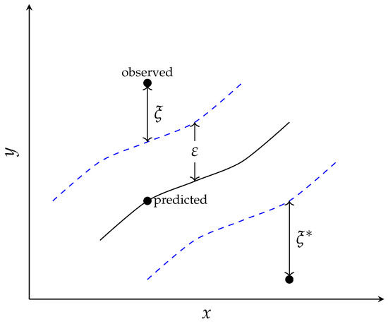
Figure 6.
The parameters for the support vector regression [26]. The solid line represents the regression function of the support vector and the dashed lines represent the error bounds of the support vector.
The optimal values of are solved by minimizing the losses and the norm of . The objective function is therefore given by Equation (4):
where ℓ is the total number of instances used in training, C, the regularization constant, is the nonzero positive value that determines the trade-off between the error and the norm of . A large value of C emphasizes the error more than the norm while a smaller value of C emphasizes the norm more. The objective function is constrained by the set of equations in Equation (5) [26]:
The SVR Model was constructed using the support vector machine (SVM) module in Scikit-learn.
2.3.5. RFR Model
Random forest is an ensemble of independent decision trees built from identically distributed datasets [27]. The dataset that is used in building each tree is randomly sampled from the training dataset with replacement. The size of the sampled dataset equals the size of the original training dataset. Random forest for regression is constructed based on numerical inputs and outputs, unlike random forest for classification which is constructed based on class labels [27].
The strength of a random forest is that the collective vote of the decision trees in the forest increases the overall accuracy and reduces the tendency of overfitting as opposed to a single decision tree which tends to easily overfit on the training dataset. For regression, voting is performed by finding the unweighted average output of all the decision trees. The larger the number of decision trees, the better the accuracy of the random forest model. However, the accuracy peaks with an increase in decision trees. Also, because a large number of decision trees requires a longer training time, it is important to find an optimal number of decision trees in the forest to balance out the training time and accuracy of the random forest.
2.4. Hyperparameter Tuning
Hyperparameter tuning is the process of strategically adjusting the model hyperparameters to determine their optimum values. Model hyperparameters are specific variables that define the configuration and behavior of a machine learning model. These variables are set by the developer before the learning process and cannot be directly estimated from data [30]. Examples of hyperparameters include the learning rate of an artificial neural network, the regularization constant of an SVR, and the number of estimators in a random forest.
The training and testing datasets (Section 2.2.3) were combined to form the hyperparameter tuning dataset. We tuned the model hyperparameters using the random search strategy [31]. The random search involved the assessment of different combinations of hyperparameter values randomly chosen from specific ranges (Table 2). For each model and lead time step, the best out of 100 different hyperparameter combinations were used to build the model for training. The hyperparameter combinations were ranked based on the mean square error (MSE) metric. We conducted the hyperparameter tuning using the KerasTuner Python package.
Table 2.
The ranges of model hyperparameters assessed during the hyperparameter tuning process.
Model Training
Apart from model hyperparameters, there are parameters that are estimated from data when training the model. These model parameters are the model’s internal variables that are not often set manually. Examples of model parameters include the weights of an artificial neural network such as LSTM. After building the models with their corresponding best hyperparameters, each model was trained on the training set.
The training processes of the LSTM 1 and LSTM 2 models were optimized using the Adam optimizer [32] with learning rates obtained from the hyperparameter tuning and an objective function of the LSTM models was to minimize the MSE. An early stopping criterion was set to terminate the training process after no change in MSE greater than 0.001 is observed during ten consecutive epochs of training. Apart from the selected hyperparameters, default settings were used in training the SVR and RFR models. All the models were trained using the training dataset (Section 2.2.3).
2.5. Model Evaluation
The models were evaluated using the testing and inference dataset (Section 2.2.3). The inference dataset was used to assess the models’ performances on a consecutive dataset. The metrics used in evaluating the models include MSE (Equation (6)), percent bias (PBIAS; Equation (7)), Nash–Sutcliffe efficiency (NSE; Equation (8)), coefficient of determination (R2; Equation (9)), and MAE (Equation (10)):
where represents the ground truth observations, represents the model output, and N is the total number of instances in the test dataset.
The R2, ranging from 0 to 1, is a measure of the degree of collinearity between the predicted and actual water level values. values close to 1 indicate less error variance between the model outputs and the actual water levels. Acceptable R2 values are greater than 0.5 [33]. The NSE is a measure of how well a model’s output fits the actual observations on a 1:1 line. The NSE ranges from to an optimal value of 1.0. The PBIAS indicates the tendency of the predicted water levels to be larger or smaller than the actual water levels. A PBIAS value close to the optimum value of 0.0% signifies an accurate model. A positive PBIAS value represents a model underestimation, while a negative value represents a model overestimation [33]. The MSE and MAE are error indices that describe the magnitude of error between the predicted and actual water level values. For any model, the closer the error index is to 0, the better the model’s performance.
The performance of the models in generating timely peak water depths was assessed by comparing the peak times in the observed water depth and the forecast peaks. The magnitudes of the peaks were compared using a percentage peak difference similar to the PBIAS but only for the peak values in context.
2.5.1. Inclusion of Rainfall Data
With an increasing trend in climate change, extreme rainfall events will consequently increase the potential of rainfall-induced floods [34,35,36]. Despite rainfall being a primary driver of runoff processes, rainfall data, including DR-RF-TD and HP-RF-TD, did not show a strong correlation with the downstream water depth C1-WD-TT, as will be seen in Section 3.1. The influence of rainfall data was tested based on the NSE, percent peak difference, and peak delay. The first test was conducted by combining only DR-RF-TD with the strongly correlated input data to generate water level forecasts. Secondly, only HP-RF-TD was combined with the strongly correlated input data to generate water level forecasts. Finally, both DR-RF-TD and HP-RF-TD were combined with the strongly correlated data to generate water level forecasts.
2.5.2. Test on the Cumberland River at Ashland City, Tennessee
After the implementation of the various machine learning models on Window Cliffs, we followed the same methodology to test the LSTM 2 model on the Cumberland River at Ashland City, Tennessee, to ascertain the effect of data quantity on the performance of the forecasting system. Compared to Window Cliffs, the Cumberland river basin has a rich collection of gauge stations with longer periods of historic data. Data from 1 January 2019, 00:00 to 31 December 2021, 23:00 were used as training and testing datasets at the Cumberland River while the inference dataset covered the period from 1 January 2022, 00:00 to 4 June 2022, 01:00.
The available data were obtained from the United States Geological Survey (USGS) and United States Army Corps of Engineers (USACE) in the form of either stage or flow hydrographs (Table 3).
Table 3.
The available sources of data within the Cumberland river basin in Tennessee.
2.6. Flood Forecasting Interface
A platform for forecasting with the trained model was developed using Jupyter Notebook [37]. This platform assimilates data in a specific format to forecast water depth at C1. The ultimate goal of the flood forecasting system is to automate the entire forecasting process. This will involve the process of automatically fetching and preparing the input dataset before generating forecasts with the trained model. However, the automation process requires extra expertise beyond the scope of this study.
3. Results
3.1. Data Collection and Preparation
The set of data that showed a strong correlation () with a water depth at C1 at time includes C1-WD-TT, DR-WL-TD, DR-WS-TT, WC-AP-TT, and WC-WL-TD. These data indicate a strong correlation from time back in time up to . To limit the size of the input data, only data from to were selected as inputs. The detailed results of the initial Spearman’s ranked correlation analyses are presented in Appendix C.
As indicated in Figure 7, there was a perfect positive association between C1-WD-TT and C1-DP-TT because C1-WD-TT is directly derived from C1-DP-TT. C1-WD-TT and C1-DP-TT both showed a strong correlation () with C1-AP-TT. C1-AP-TT and C1-DP-TT were therefore dropped from the set of selected input data. C1-WD-TT was maintained with the intuition that a historic water depth at C1 is likely a good factor in determining the future water depth at C1. WC-WL-TD, DR-WL-TD, and DR-WS-TT were maintained despite their strong cross-correlation () because they were recorded at different locations and with different recording systems unlike data from C1 which were all measured with one device and at the same location.
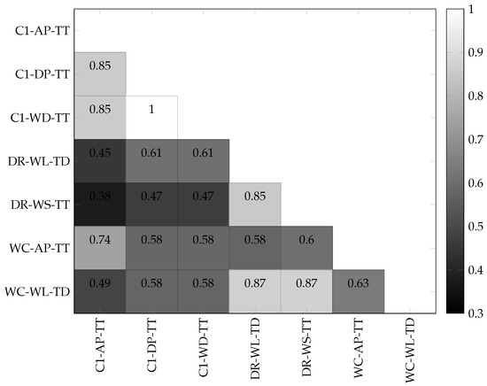
Figure 7.
Cross-correlation between predictor variables.
3.2. Machine Learning Model Development
The hyperparameters for each model architecture and the lead time steps of 3 h, 4 h, 5 h, and 6 h were determined using a random search strategy. Table 4 shows the selected hyperparameters for each model architecture and the corresponding lead time step. The MSE values measured during the hyperparameter tuning were the bases for model configuration selection. The selected model hyperparameters were then used to build the models for training.
Table 4.
Hyperparameter tuning results for the best configurations for lead times of six, five, four, and three hours. Further details on ranked hyperparameter tuning results are presented in Appendix D.
3.3. Model Evaluation
Evaluation of the test dataset showed that the RFR model yielded the lowest ranges of errors such as – m2 MSE and – m MAE (Figure 8a). The positive range of PBIAS in the LSTM 1, RFR, and SVR indicates that these models have higher tendencies to underpredict than the LSTM 2 models which showed a negative PBIAS of −2.408% and −0.604% for the 3 h and 4 h lead times, respectively. The LSTM 1, RFR, and SVR models had a range of PBIAS from 1.334% (3 h LSTM 1) to 5.890% (6 h SVR). However, for the LSTM 2 model, a sharp increase in PBIAS from 0.114% in a 5 h lead time to 11.461% in a 6 h lead time. The RFR model yielded the best similarity in pattern in terms of the NSE with minimum and maximum values of 0.576 (4 h lead time) and 0.760 (3 h lead time), respectively. The RFR models’ R2 on the testing dataset ranged from 0.584 (4 h lead time) to 0.774 (3 h lead time) as shown in Figure 8a.
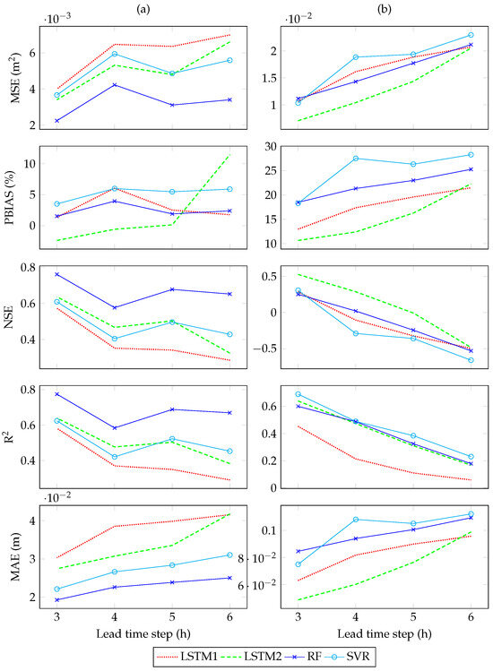
Figure 8.
Model performance on the (a) testing dataset (left column) and (b) inference dataset (right column). The variation in the model performance is plotted with an increasing order of lead time. Further details are presented in Appendix E.
In general, the evaluation of the testing dataset indicated a better performance than the inference data. For example, the range of MSE in the testing dataset is from 0.024 (3 h RFR) to 0.075 (6 h LSTM 1) whereas the MSE ranged from 0.076 (3 h LSTM 2) to 0.228 (6 h RFR) in the inference dataset (Figure 8; Table A6). However, a consistent improvement in performance with a reduction in lead time was seen across all models when tested on the inference dataset. From the inference dataset, only the LSTM 2 model with a 3 h lead time yielded an NSE value of 0.526, greater than the recommended value of 0.5 [33]. At most times, all the models underpredicted in the inference dataset with a positive PBIAS values ranging from 10.654% (3 h LSTM 2) to 28.274% (6 h SVR). While the LSTM 2, RFR, and SVR models yielded similar ranges of R2 with differences ranging from 0.015 to 0.089, the LSTM 1 model consistently yielded a lower R2 than the other models in all lead times with a minimum value of 0.059 (6 h lead time) and a maximum value of 0.453 (3 h lead time) as shown in Figure 8b.
The LSTM 2 model yielded the closest approximation of the inference hydrograph’s peak with percent peak difference values ranging from 8.2% for a 3 h lead time to 22.5% for a 6 h lead time (Table 5; Figure 9). The highest percent peak difference of 37.3% was observed in the LSTM 1 model for the 6 h lead time. Overall, the positive percent peak differences indicate that all the models forecast peak values lower than the actual peak. Another important performance indicator worth noting is the delay in the time to peak. For all the models, the higher the lead time, the longer the delay in the peak forecast (Table 5). The SVR model yielded the shortest delay of 2 h for the 3 h and 4 h lead times. The LSTM 1 model resulted in the longest delays ranging from 8 h for a 3 h lead time to 12 h for a 6 h lead time.
Table 5.
Analysis of the time to peak using the inference dataset.
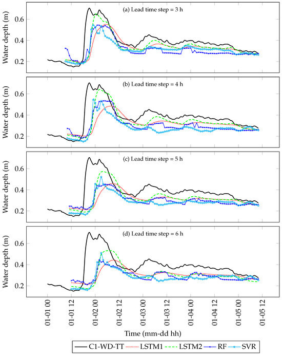
Figure 9.
Inference from 1 January 2022, 00:00 to 5 January 2022, 10:00 based on (a) 3 h; (b) 4 h; (c) 5 h; and (d) 6 h lead time steps.
3.3.1. Inclusion of Rainfall Data
The available rainfall data were combined with the selected, strongly correlated data (Section 3.1) in three different ways to generate forecasts: (1) combining only DR-RF-TD; (2) combining only HP-RF-TD; and (3) combining both DR-RF-TD and HP-RF-TD. The results were evaluated based on the NSE, percent peak difference, and peak delay. For each metric, the best- and worst-performing models during the initial model evaluation (Section 3.3) were selected for further assessment. In terms of NSE, the 3 h RFR and 6 h LSTM 1 were selected while the 3 h LSTM 2 and 6 h LSTM 1 were selected for the percent peak difference. For the peak delay, the 3 h SVR and 6 h LSTM 1 were selected.
The addition of only DR-RF-TD to the strongly correlated data resulted in an improvement in NSE from 0.760 to 0.774 for the 3 h RFR and 0.285 to 0.292 for the 6 h LSTM 1 (Table 6). Adding only HP-RF-TD to the strongly correlated data yielded an improved NSE of 0.765 and 0.299 for the 3 h RFR and 6 h LSTM 1, respectively. When both DR-RF-TD and HP-RF-TD were combined with the selected, strongly correlated data, the 3 h RFR yielded a stronger NSE of 0.785 while the NSE of the 6 h LSTM 1 was reduced to 0.263 (Table 6).
Table 6.
NSE comparison of different combinations of rainfall data.
While combining only DR-RF-TD with the strongly correlated data did not change the peak delay in the 3 h SVR and 6 h LSTM 1, combining only HP-RF-TD reduced the peak delay in both models by 1 h. Including both DR-RF-TD and HP-RF-TD further reduced the peak delay of the 6 h LSTM 1 to 10 h while the peak delay was reduced to 1 h in the 3 h SVR (Table 7).
Table 7.
Peak delay comparison of different combinations of rainfall data.
In terms of percent peak difference, the 3 h LSTM 2 and 6 h LSTM were assessed (Table 8). Combining DR-RF-TD with the strongly correlated data resulted in a reduction in percent peak difference for both the 3 h LSTM 2 and the 6 h LSTM 1. The 3 h LSTM 2 yielded a percent peak difference of 6.2% and the 6 h LSTM 1 yielded a percent peak difference of 35.9%. The 3 h LSTM 2 saw an increase in the percent peak difference from 8.2% to 11.2 when only HP-RF-TD was combined with the strongly correlated data. Meanwhile, the 6 h LSTM 1 saw an improvement when only the HP-RF-TD was included. Combining both DR-RF-TD and DR-RF-TD increased the percent peak difference to 8.3% and 38.6% for the 3 h LSTM 2 and 6 h LSTM 1, respectively, (Table 8).
Table 8.
Percent peak difference comparison of different combinations of rainfall data.
3.3.2. Test on the Cumberland River at Ashland City, Tennessee
The LSTM 2 model was tested on the Cumberland River at Ashland City with the following hyperparameters: 180 LSTM units, 70 dense units, 3 dense layers, and a learning rate of 0.033334. The hyperparameters were selected using a random search strategy. A comparison between observed and forecast stage values showed a near-perfect similarity with NSE values of 0.980 and 0.970 for the testing and inference datasets, respectively. The testing and inference datasets also yielded R2 values of 0.980 and 0.970, respectively. The negative PBIAS values close to the optimum value of 0.0% indicate that the forecast values were mostly not significantly greater than the observed stage values (Table 9).
Table 9.
Performance of the LSTM 2 model when tested on the Cumberland River dataset.
A comparison of peaks indicated a minuscule difference of 0.12 ft in the peak percent peak stage and a delay of 3 h on 25 February 2022 (Figure 9). However, in some instances, the LSTM 2 model overestimated the peaks. For example, on 23 February 2022, the model overestimated the peak by 0.10 ft with a 2 h delay (highlighted by a red ellipse in Figure 10).
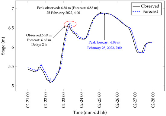
Figure 10.
Inference on the Cumberland River from 21 February 2022, 00:00 to 27 February 2022, 23:00 using a 3 h LSTM 2 model. The plotted hydrographs show the observed and forecast peak stages during the inference period.
3.4. Flood Forecasting Interface
We developed a graphical user interface (GUI) for the flood forecasting system with the option to select a model architecture and a lead time step. When the input data are uploaded, a hydrograph of the historic water levels at C1 is displayed (solid blue line; Figure 11). The forecast button generates the forecast water level(s) at C1 which is appended to the historic hydrograph as a “dash-dotted” orange line. Because they generate a single output value, the LSTM 1, RFR, and SVR models result in a single line connecting the last historic water depth to the forecast water level. On the other hand, the LSTM 2 model can generate intermediate values between the current water level and the forecast.
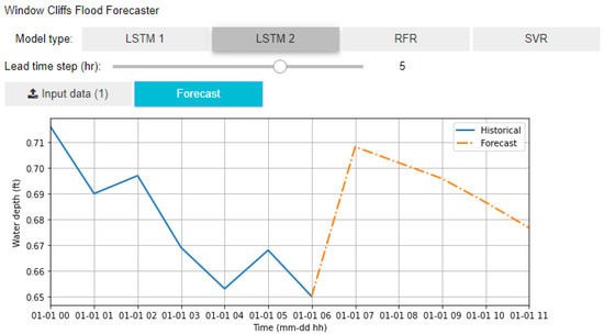
Figure 11.
GUI of the flood forecasting tool for Window Cliffs developed in Jupyter Notebook.
4. Discussion
The variations in the performance of the different models can be attributed to the differences in the model architectures. The underlying algorithms and assumptions for each model architecture contribute to the differences in performance. For example, the RFR model showed a better performance in the test dataset which may be attributed to the model’s ability to learn the nonlinearities between the input features and the target variable. However, when tested on the inference dataset, the model showed a relatively poorer performance than the LSTM 2 model. This may be attributed to the RFR’s model’s inability to generalize properly on the training dataset. LSTM models are generally suited for series datasets; hence, the LSTM 2 is well adapted for the time series dataset used in this study. The LSTM 2 model showed a better performance in the inference dataset than the RFR model. The limited amount of data used in this study may have also contributed to the reduction in the performance of the models when tested on the inference dataset.
Compared to the model performances on the testing datasets, the performances observed on the inference dataset indicated relatively higher error indices such as MSE and MAE. This is because, unlike the inference dataset, the testing dataset was drawn from the same distribution as the training dataset. Because of the limited dataset in this study, the inference dataset was selected from data that chronologically follow the training and testing datasets.
Despite the consistent positive PBIAS and percent peak difference (Table 5), the magnitude of difference indicated by a minimum of 0.063 ft (3 h RFR in the testing dataset) and a maximum of 0.368 ft (3 h SVR in the inference dataset) can be classified as insignificant. However, given the available data used in this study and the overall maximum, corrected water depth of 2.65 ft, the performance of the models cannot be ascertained for extremely high water events. For example, recently observed water depth records dated outside the time frame of the data used in this study showed an uncorrected water depth of 9.77 ft on 27 January 2022, 07:00 at C1. Such an extreme event is about 370% greater than the maximum water depth used in this study. There is therefore the need to further train and assess the performance of the models in forecasting a wide range of possible extreme events at Window Cliffs.
The performance of a machine learning model is influenced by the quantity and quality of the data used in developing the model. The two months of data used in this study do not capture most of the seasonal variations within a year. This was evident in the better performance metrics observed from the testing dataset compared to the inference dataset. The dataset used to train the models was more representative of the testing dataset than the inference dataset. Even though the data preparation process involved some techniques such as shuffling to ensure an unbiased mix of available data, at least a full year’s data would be needed to ensure that the models are trained for well-varied conditions and events.
In the forecast problem, a longer lead time is preferred since a longer lead time implies enough time to plan park closures or evacuate the park to protect lives and property. However, it was observed that increasing the lead time increased the error in forecast hydrographs. Coupled with the resulting errors, the time to peak was delayed in the forecast hydrographs by a minimum of 2 h (3 h SVR) and a maximum of 12 h (5 and 6 h LSTM 1). Such delays negate the advantage of setting enough lead time in the model.
The rainfall data did not show a strong correlation with the target water depth data downstream. The response to rainfall events at the downstream location may be delayed by the time it takes for the water to travel from the upstream location to the downstream location. The delay in the response to rainfall events may be the reason for the weak correlation results for the rainfall data. Hence, we did not include rainfall as input in the first set of simulations. However, the subsequent inclusion of rainfall data showed a promising model improvement in terms of NSE, percent peak difference, and peak delay. For example, including the various combinations of DR-RF-TD and HP-RF-TD improved the NSE values in all scenarios of the 3 h RFR and 6 h LSTM 1 except for the inclusion of both DR-RF-TD and HP-RF-TD on the 6 h LSTM 1 model (Table 6). In terms of peak delay, adding only HP-RF-TD or both DR-RF-TD and HP-RF-TD reduced the peak delay in the 3 h SVR and 6 h LSTM 1 (Table 7). The percent peak difference for the 6 h LSTM 1 reduced in all combinations of DR-RF-TD and HP-RF-TD, while only the inclusion of DR-RF-TD reduced the percentage peak difference in the 3 h LSTM 2 model (Table 8).
The LSTM 2 model, when tested on the Cumberland River with over two years of data, showed an improved performance in terms of similarity between the ground truth observations and forecast values compared to the performance at Window Cliffs. The LSTM 2 model also yielded insignificant percent errors in peak forecast. With enough data, the LSTM 2 model was able to forecast peaks with a maximum delay of 3 h and occasionally, lesser delay times. The test on the Cumberland River shows the promising performance of the forecast models when trained with more data from the Window Cliffs’ domain.
5. Conclusions
In this study, four model architectures, the LSTM 1, LSTM 2, RFR, and SVR, were used to forecast water depths at Window Cliffs creek crossing 1. The models were evaluated with lead times of 3, 4, 5, and 6 h. Overall, the evaluation of the models indicated different strengths of the different models. For example, the LSTM 2 model yielded the least percent difference with a 3 h lead time and the SVR model forecasted the peaks with shorter delays of 2 h when tested with a lead time of 3 and 4 h (Table 5). valuation of the testing dataset showed that the RFR model resulted in the lowest range of errors such as the MAE of 1.92 × –2.50 × m. The varied strengths of the various models can be combined in an ensemble model to generate more accurate forecasts. This study also highlights the importance of rainfall data in flood forecasting, mainly because rainfall is a primary trigger for flooding. The inclusion of rainfall data in the model development improved the performance of the models in terms of NSE, percent peak difference, and peak delay even though the initial correlation did not show a strong correlation between rainfall and the target water depth.
Limitations and Recommendations
The models developed in this study can be further improved by training the models with more data that cover at least one complete hydrological year. This will expose the models to a wide variety of events and capture the influence of seasonal variations within a year. With enough data to train the model, the model will cover almost all scenarios that would be seen in the inference dataset. We recommend the frequent maintenance of the gauges at Window Cliffs to ensure that the data used in training the models are of good quality and cover a wide range of events.
Apart from the quantity of data used in developing the models, the type of data involved may be a factor for the delayed peak response and higher errors related to longer lead times. For instance, adding rainfall data generally improved the models’ NSE, peak delay, and percent peak difference. Currently, the models do not factor in the influence of other future hydrologic factors such as precipitation, temperature, and wind [22]. The feasibility of including forecast datasets in the model development needs to be investigated, as including the forecast data may improve the delay in peaks and the difference in peaks.
An improvement in at least one of the models will lead to a better discrimination between the performances of the models. Without discriminable performance measures, an ensemble of the models can be explored to harness the collective strengths of the individual models.
Author Contributions
Conceptualization, G.K.D. and A.K.; methodology, G.K.D., C.O. and A.K.; software, G.K.D.; validation, G.K.D.; formal analysis, G.K.D. and C.O.; investigation, G.K.D. and A.K.; resources, A.K.; data curation, G.K.D. and C.O.; writing—original draft preparation, G.K.D.; writing—review and editing, A.K. and C.O.; visualization, G.K.D.; supervision, A.K.; project administration, A.K.; funding acquisition, A.K. All authors have read and agreed to the published version of the manuscript.
Funding
This research received no external funding. The authors acknowledge the funding and administrative support from the Center for the Management, Utilization, Protection of Water Resources (TNTech Water Center) at the Tennessee Technological University.
Institutional Review Board Statement
Not applicable.
Data Availability Statement
The data files and code used in this study can be accessed on GitLab at https://gitlab.csc.tntech.edu/gkdarkwah42/flood-forecasting-model.git upon request. Requests should be sent to the corresponding author at akalyanapu@tntech.edu.
Acknowledgments
The authors would like to acknowledge the support from the Tennessee Department of Environment and Conservation, Tennessee State Parks, and Friends of Burgess Falls. The authors would also like to acknowledge the hard work and dedication of the following TNTech students (who have graduated): Alex Davis, Chris Kaczmarek, and Devin Rains.
Conflicts of Interest
The authors declare no conflicts of interest. The funders had no role in the design of the study; in the collection, analyses, or interpretation of data; in the writing of the manuscript; or in the decision to publish the results.
Abbreviations
The following abbreviations are used in this manuscript:
| FEWS | Flood early warning system |
| GUI | Graphical user interface |
| HUC | Hydrologic unit code |
| LASSO | Least absolute shrinkage and selection operator |
| LSTM | Long short-term memory |
| MAE | Mean absolute error |
| MSE | Mean squared error |
| NSE | Nash–Sutcliffe model efficiency coefficient |
| NWS | National Weather Service |
| PBIAS | Percent bias |
| RF | Random forest |
| RFC | River forecasting center |
| RFR | Random forest regression |
| SVR | Support vector regression |
| TDEC | Tennessee Department of Environment and Conservation |
| TTU | Tennessee Technological University |
| U.S. | United States |
| USACE | United States Army Corp of Engineers |
| USGS | United States Geological Survey |
Appendix A. Data Availability Chart
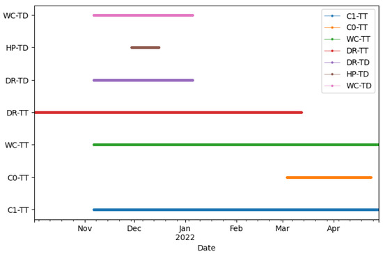
Figure A1.
The data availability chart for the gauge locations within the Cane Creek watershed. Legend description: C1-TT-TTU gauge at Creek Crossing 1; C0-TT-TTU gauge at Creek Crossing 10; WC-TT-TTU gauge at Window Cliffs Road; DR-TT-TTU gauge at Ditty Lane; DR-TD-TDEC gauge at Ditty Lane; HP-TD-TDEC gauge at Highland Park Boulevard; WC-TD-TDEC gauge at Window Cliffs Road.
Appendix B. Distribution of Input Features
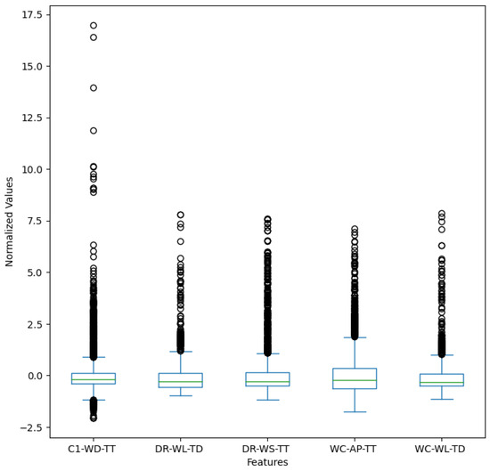
Figure A2.
Distribution of the normalized input features. The data were normalized and centered at zero by subtracting the mean and dividing by the standard deviation. The black circles represent outliers in the dataset for each location.
Appendix C. Spearman’s Ranked Correlation Analysis
Table A1.
Spearman correlation between the water depth at Creek Crossing 1 (C1-WD-TT) and the available historical data up to 7 timesteps back in history.
Table A1.
Spearman correlation between the water depth at Creek Crossing 1 (C1-WD-TT) and the available historical data up to 7 timesteps back in history.
| Data Location | Historical Timesteps (h) | |||||||
|---|---|---|---|---|---|---|---|---|
| t − 0 | t − 1 | t − 2 | t − 3 | t − 4 | t − 5 | t − 6 | t − 7 | |
| C1-AP-TT | 0.63 | 0.60 | 0.58 | 0.56 | 0.54 | 0.52 | 0.51 | 0.49 |
| C1-BP-TT | 0.15 | 0.14 | 0.13 | 0.12 | 0.11 | 0.11 | 0.10 | 0.09 |
| C1-DP-TT | 0.72 | 0.68 | 0.65 | 0.63 | 0.61 | 0.59 | 0.57 | 0.55 |
| C1-TP-TT | −0.05 | −0.01 | 0.02 | 0.04 | 0.06 | 0.07 | 0.07 | 0.08 |
| C1-WD-TT | 0.72 | 0.68 | 0.65 | 0.63 | 0.61 | 0.59 | 0.57 | 0.55 |
| DR-RF-TD | 0.19 | 0.20 | 0.21 | 0.21 | 0.21 | 0.22 | 0.21 | 0.20 |
| DR-WL-TD | 0.57 | 0.56 | 0.56 | 0.56 | 0.55 | 0.55 | 0.54 | 0.54 |
| DR-WS-TT | 0.59 | 0.60 | 0.61 | 0.62 | 0.62 | 0.62 | 0.62 | 0.61 |
| HP-RF-TD | 0.05 | 0.06 | 0.07 | 0.08 | 0.07 | 0.06 | 0.05 | 0.04 |
| WC-AP-TT | 0.55 | 0.55 | 0.54 | 0.54 | 0.53 | 0.52 | 0.52 | 0.51 |
| WC-BP-TT | 0.14 | 0.13 | 0.12 | 0.12 | 0.11 | 0.10 | 0.10 | 0.09 |
| WC-DP-TT | 0.41 | 0.41 | 0.41 | 0.41 | 0.41 | 0.41 | 0.41 | 0.41 |
| WC-TP-TT | −0.17 | −0.15 | −0.13 | −0.12 | −0.11 | −0.10 | −0.09 | −0.08 |
| WC-WD-TT | 0.41 | 0.41 | 0.41 | 0.41 | 0.41 | 0.41 | 0.41 | 0.41 |
| WC-WL-TD | 0.55 | 0.56 | 0.57 | 0.58 | 0.58 | 0.58 | 0.59 | 0.59 |
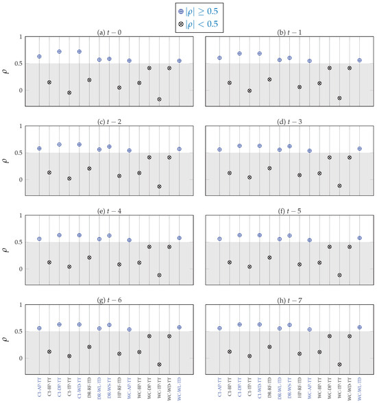
Figure A3.
Spearman’s ranked correlation analysis. We generated the plots using data from Table A1.
Appendix D. Hyperparameter Tuning Results
Table A2.
Hyperparameter tuning results for the best five configurations with a lead time of 3 h.
Table A2.
Hyperparameter tuning results for the best five configurations with a lead time of 3 h.
| Model | Hyperparameter (Hypertune Metric) | Rank | ||||
|---|---|---|---|---|---|---|
| 1st | 2nd | 3rd | 4th | 5th | ||
| LSTM 1 | No. of LSTM units | 90 | 50 | 110 | 50 | 170 |
| No. of dense units | 180 | 140 | 140 | 230 | 130 | |
| No. of dense layers | 4 | 5 | 1 | 3 | 2 | |
| Learning rate | 0.0560 | 0.0810 | 0.0960 | 0.0660 | 0.0960 | |
| (MSE [ m2]) | 2.211 | 2.230 | 2.230 | 2.239 | 2.239 | |
| LSTM 2 | No. of LSTM units | 25 | 115 | 330 | 25 | 100 |
| No. of dense units | 390 | 265 | 300 | 415 | 355 | |
| No. of ense layers | 2 | 3 | 1 | 4 | 1 | |
| Learning rate | 0.0945 | 0.0937 | 0.0927 | 0.0939 | 0.0728 | |
| (MSE [ m2]) | 0.0316 | 0.0318 | 0.0319 | 0.0321 | 0.0323 | |
| RFR | No. of estimators | 161 | 175 | 163 | 127 | 85 |
| (MSE [ m2]) | 1.384 | 1.384 | 1.384 | 1.394 | 1.394 | |
| SVR | Epsilon | 0.0406 | 0.0502 | 0.0684 | 0.0880 | 0.0739 |
| C | 1.3137 | 7.4276 | 7.9804 | 9.0464 | 6.5188 | |
| (MSE [ m2]) | 2.025 | 2.025 | 2.025 | 2.025 | 2.035 | |
Table A3.
Hyperparameter tuning results for the best five configurations with a lead time of 4 h.
Table A3.
Hyperparameter tuning results for the best five configurations with a lead time of 4 h.
| Model | Hyperparameter (Hypertune Metric) | Rank | ||||
|---|---|---|---|---|---|---|
| 1st | 2nd | 3rd | 4th | 5th | ||
| LSTM 1 | No. of LSTM units | 20 | 150 | 20 | 80 | 20 |
| No. of dense units | 140 | 120 | 160 | 140 | 230 | |
| No. of dense layers | 5 | 2 | 1 | 2 | 1 | |
| Learning rate | 0.0710 | 0.0960 | 0.0760 | 0.0860 | 0.0960 | |
| (MSE [ m2]) | 2.806 | 2.824 | 2.843 | 2.852 | 2.852 | |
| LSTM 2 | No. of LSTM units | 385 | 275 | 60 | 45 | 500 |
| No. of dense units | 400 | 60 | 405 | 335 | 70 | |
| No. of dense layers | 1 | 5 | 1 | 6 | 3 | |
| Learning rate | 0.0969 | 0.0931 | 0.0768 | 0.0984 | 0.0915 | |
| (MSE [ m2]) | 4.534 | 4.562 | 4.580 | 4.580 | 4.580 | |
| RFR | No. of estimators | 155 | 100 | 157 | 166 | 130 |
| (MSE [ m2]) | 1.682 | 1.682 | 1.691 | 1.691 | 1.691 | |
| SVR | Epsilon | 0.0543 | 0.1104 | 0.0253 | 0.0326 | 0.1026 |
| C | 7.7472 | 9.2149 | 4.0142 | 6.6004 | 7.2953 | |
| (MSE [ m2]) | 2.564 | 2.564 | 2.573 | 2.573 | 2.573 | |
Table A4.
Hyperparameter tuning results for the best five configurations with a lead time of 5 h.
Table A4.
Hyperparameter tuning results for the best five configurations with a lead time of 5 h.
| Model | Hyperparameter (Hypertune Metric) | Rank | ||||
|---|---|---|---|---|---|---|
| 1st | 2nd | 3rd | 4th | 5th | ||
| LSTM 1 | No. of LSTM units | 30 | 50 | 60 | 80 | 140 |
| No. of dense units | 100 | 60 | 70 | 250 | 280 | |
| No. of dense layers | 2 | 2 | 4 | 2 | 4 | |
| Learning rate | 0.0460 | 0.0860 | 0.0910 | 0.0710 | 0.0860 | |
| (MSE [ m2]) | 3.317 | 3.363 | 3.372 | 3.372 | 3.391 | |
| LSTM 2 | No. of LSTM units | 195 | 305 | 115 | 35 | 370 |
| No. of dense units | 240 | 65 | 240 | 380 | 280 | |
| No. of dense layers | 2 | 1 | 4 | 6 | 7 | |
| Learning rate | 0.0853 | 0.0802 | 0.0880 | 0.0666 | 0.0965 | |
| (MSE [ m2]) | 6.680 | 6.773 | 6.773 | 6.782 | 6.801 | |
| RFR | No. of estimators | 83 | 163 | 161 | 149 | 72 |
| (MSE [ m2]) | 1.747 | 1.774 | 1.774 | 1.784 | 1.793 | |
| SVR | Epsilon | 0.0773 | 0.0675 | 0.0585 | 0.0218 | 0.0545 |
| C | 8.9307 | 9.9592 | 5.5814 | 9.3182 | 5.2299 | |
| (MSE [ m2]) | 2.899 | 2.908 | 2.926 | 2.964 | 2.964 | |
Table A5.
Hyperparameter tuning results for the best five configurations with a lead time of 6 h.
Table A5.
Hyperparameter tuning results for the best five configurations with a lead time of 6 h.
| Model | Hyperparameter (Hypertune Metric) | Rank | ||||
|---|---|---|---|---|---|---|
| 1st | 2nd | 3rd | 4th | 5th | ||
| LSTM 1 | No. of LSTM units | 30 | 60 | 20 | 190 | 80 |
| No. of dense units | 30 | 210 | 250 | 90 | 90 | |
| No. of dense layers | 3 | 3 | 3 | 2 | 4 | |
| Learning rate | 0.0610 | 0.0860 | 0.0960 | 0.0860 | 0.0710 | |
| (MSE [ m2]) | 3.735 | 3.753 | 3.800 | 3.809 | 3.837 | |
| LSTM 2 | No. of LSTM units | 205 | 455 | 305 | 85 | 335 |
| No. of dense units | 150 | 350 | 110 | 220 | 315 | |
| No. of dense layers | 2 | 5 | 1 | 2 | 1 | |
| Learning rate | 0.0964 | 0.0869 | 0.0721 | 0.0915 | 0.0918 | |
| (MSE [ m2]) | 9.235 | 9.262 | 9.290 | 9.300 | 9.327 | |
| RFR | No. of estimators | 183 | 61 | 191 | 166 | 97 |
| (MSE [ m2]) | 1.858 | 1.858 | 1.867 | 1.877 | 1.877 | |
| SVR | Epsilon | 0.0758 | 0.0801 | 0.0615 | 0.0679 | 0.0467 |
| C | 8.8529 | 7.3196 | 7.3582 | 6.6954 | 7.2667 | |
| (MSE [ m2]) | 3.214 | 3.224 | 3.233 | 3.242 | 3.242 | |
Appendix E. Model Evaluation Results
Table A6.
Evaluation of the testing and inference datasets using the MSE, PBIAS, NSE, R2, and MAE metrics.
Table A6.
Evaluation of the testing and inference datasets using the MSE, PBIAS, NSE, R2, and MAE metrics.
| Evaluation Metric | Model | Testing Dataset | Inference Dataset | ||||||
|---|---|---|---|---|---|---|---|---|---|
| 3 h | 4 h | 5 h | 6 h | 3 h | 4 h | 5 h | 6 h | ||
| MSE ( m2) | LSTM 1 | 3.995 | 6.503 | 6.317 | 6.968 | 10.684 | 16.165 | 18.859 | 20.717 |
| LSTM 2 | 3.437 | 5.295 | 4.831 | 6.596 | 7.061 | 10.405 | 14.307 | 20.532 | |
| RFR | 2.230 | 4.274 | 3.159 | 3.437 | 11.148 | 14.307 | 17.744 | 21.182 | |
| SVR | 3.623 | 5.946 | 4.831 | 5.574 | 10.312 | 18.859 | 19.324 | 22.947 | |
| PBIAS (%) | LSTM 1 | 1.334 | 6.048 | 2.509 | 1.748 | 12.976 | 17.374 | 19.576 | 21.467 |
| LSTM 2 | −2.408 | −0.604 | 0.114 | 11.461 | 10.654 | 12.408 | 16.281 | 22.289 | |
| RFR | 1.520 | 3.945 | 1.889 | 2.379 | 18.496 | 21.325 | 22.989 | 25.266 | |
| SVR | 3.502 | 5.984 | 5.468 | 5.890 | 18.289 | 27.512 | 26.324 | 28.274 | |
| NSE | LSTM 1 | 0.573 | 0.352 | 0.341 | 0.285 | 0.286 | −0.105 | −0.323 | −0.496 |
| LSTM 2 | 0.637 | 0.467 | 0.503 | 0.325 | 0.526 | 0.287 | −0.007 | −0.483 | |
| RFR | 0.760 | 0.576 | 0.677 | 0.652 | 0.252 | 0.021 | −0.244 | −0.530 | |
| SVR | 0.609 | 0.405 | 0.496 | 0.428 | 0.307 | −0.290 | −0.359 | −0.659 | |
| R2 | LSTM 1 | 0.581 | 0.370 | 0.350 | 0.290 | 0.453 | 0.214 | 0.110 | 0.059 |
| LSTM 2 | 0.639 | 0.477 | 0.503 | 0.383 | 0.639 | 0.474 | 0.311 | 0.168 | |
| RFR | 0.774 | 0.584 | 0.688 | 0.669 | 0.600 | 0.488 | 0.325 | 0.179 | |
| SVR | 0.624 | 0.421 | 0.522 | 0.453 | 0.689 | 0.489 | 0.384 | 0.231 | |
| MAE ( m) | LSTM 1 | 3.048 | 3.840 | 3.993 | 4.145 | 6.279 | 8.169 | 8.992 | 9.571 |
| LSTM 2 | 2.743 | 3.078 | 3.353 | 4.176 | 4.846 | 6.005 | 7.650 | 9.876 | |
| RFR | 1.920 | 2.256 | 2.377 | 2.499 | 8.443 | 9.388 | 10.058 | 10.942 | |
| SVR | 2.225 | 2.652 | 2.835 | 3.109 | 7.498 | 10.820 | 10.516 | 11.217 | |
Appendix F. Evaluation Results with Rainfall Data
Table A7.
Evaluation of different combinations of rainfall data with selected and strongly correlated data.
Table A7.
Evaluation of different combinations of rainfall data with selected and strongly correlated data.
| Included Rainfall | Model | NSE | % Peak Difference | Peak Delay (h) |
|---|---|---|---|---|
| DR-RF-TD only | 6 h LSTM 1 | 0.292 | 35.9 | 12 |
| 3 h LSTM 2 | 0.589 | 6.2 | 4 | |
| 3 h RFR | 0.774 | 21.1 | 4 | |
| 3 h SVR | 0.613 | 22.1 | 2 | |
| HP-RF-TD only | 6 h LSTM 1 | 0.299 | 35.0 | 11 |
| 3 h LSTM 2 | 0.603 | 11.2 | 4 | |
| 3 h RFR | 0.765 | 23.5 | 5 | |
| 3 h SVR | 0.617 | 19.2 | 1 | |
| DR-RF-TD and HP-RF-TD | 6 h LSTM 1 | 0.263 | 38.6 | 13 |
| 3 h LSTM 2 | 0.586 | 8.3 | 6 | |
| 3 h RFR | 0.785 | 21.6 | 10 | |
| 3 h SVR | 0.607 | 18.0 | 1 |
References
- Svetlana, D.; Radovan, D.; Ján, D. The Economic Impact of Floods and their Importance in Different Regions of the World with Emphasis on Europe. Procedia Econ. Financ. 2015, 34, 649–655. [Google Scholar] [CrossRef]
- Teng, J.; Jakeman, A.J.; Vaze, J.; Croke, B.F.; Dutta, D.; Kim, S. Flood inundation modelling: A review of methods, recent advances and uncertainty analysis. Environ. Model. Softw. 2017, 90, 201–216. [Google Scholar] [CrossRef]
- Smith, A.B. U.S. Billion-Dollar Weather and Climate Disasters, 1980—Present (NCEI Accession 0209268). Version 4.4. NOAA National Centers for Environmental Information. Dataset. 2020. Available online: https://www.ncei.noaa.gov/access/metadata/landing-page/bin/iso?id=gov.noaa.nodc:0209268 (accessed on 10 December 2020).
- Ready. 2018. Available online: https://www.ready.gov/floods (accessed on 10 December 2020).
- Mosavi, A.; Ozturk, P.; Chau, K.W. Flood Prediction Using Machine Learning Models: Literature Review. Water 2018, 10, 1536. [Google Scholar] [CrossRef]
- Di Baldassarre, G.; Schumann, G.; Bates, P.D.; Freer, J.E.; Beven, K.J. Flood-plain mapping: A critical discussion of deterministic and probabilistic approaches. Hydrol. Sci. J. 2010, 55, 364–376. [Google Scholar] [CrossRef]
- Pashazadeh, A.; Javan, M. Comparison of the gene expression programming, artificial neural network (ANN), and equivalent Muskingum inflow models in the flood routing of multiple branched rivers. Theor. Appl. Climatol. 2020, 139, 1349–1362. [Google Scholar] [CrossRef]
- Solomatine, D.P.; Ostfeld, A. Data-driven modelling: Some past experiences and new approaches. J. Hydroinform. 2008, 10, 3–22. [Google Scholar] [CrossRef]
- Nguyen, T.T.; Huu, Q.N.; Li, M.J. Forecasting Time Series Water Levels on Mekong River Using Machine Learning Models. In Proceedings of the Proceedings—2015 IEEE International Conference on Knowledge and Systems Engineering (KSE), Ho Chi Minh City, Vietnam, 8–10 October 2015; pp. 292–297. [Google Scholar] [CrossRef]
- Mitchell, T. Machine Learning; McGraw-Hill Series in Computer Science; McGraw-Hill: New York, NY, USA, 1997. [Google Scholar]
- Ghorpade, P.; Gadge, A.; Lende, A.; Chordiya, H.; Gosavi, G.; Mishra, A.; Hooli, B.; Ingle, Y.S.; Shaikh, N. Flood Forecasting Using Machine Learning: A Review. In Proceedings of the 2021 8th International Conference on Smart Computing and Communications (ICSCC), Kochi, Kerala, India, 1–3 July 2021; pp. 32–36. [Google Scholar] [CrossRef]
- Nevo, S.; Morin, E.; Gerzi Rosenthal, A.; Metzger, A.; Barshai, C.; Weitzner, D.; Voloshin, D.; Kratzert, F.; Elidan, G.; Dror, G.; et al. Flood forecasting with machine learning models in an operational framework. Hydrol. Earth Syst. Sci. 2022, 26, 4013–4032. [Google Scholar] [CrossRef]
- Frame, J.M.; Kratzert, F.; Klotz, D.; Gauch, M.; Shalev, G.; Gilon, O.; Qualls, L.M.; Gupta, H.V.; Nearing, G.S. Deep learning rainfall–runoff predictions of extreme events. Hydrol. Earth Syst. Sci. 2022, 26, 3377–3392. [Google Scholar] [CrossRef]
- Adams, T.E. Chapter 10—Flood Forecasting in the United States NOAA/National Weather Service; Academic Press: Boston, UK, 2016; pp. 249–310. [Google Scholar] [CrossRef]
- McEnery, J.; Ingram, J.; Duan, Q.; Adams, T.; Anderson, L. NOAA’S Advanced Hydrologic Prediction Service: Building Pathways for Better Science in Water Forecasting. Bull. Am. Meteorol. Soc. 2005, 86, 375–386. [Google Scholar] [CrossRef]
- NOAA. NOAA—National Weather Service—Water. Available online: https://water.weather.gov/ahps/forecasts.php (accessed on 5 November 2021).
- Alund, N.N. After Flooding Deaths at Cummins Falls, NWS Ramps up Communication Efforts. The Tennessean. 2017. Available online: https://www.tennessean.com/story/news/2017/08/17/after-flooding-deaths-cummins-falls-nws-ramps-up-communication-efforts/575550001/ (accessed on 20 January 2021).
- Dance, B. Floods at Cummins Falls: What Safety Measures Are in Place? The Tennessean. 2019. Available online: https://www.tennessean.com/story/news/2019/06/10/cummins-falls-tn-park-flood-safety/1408288001 (accessed on 20 January 2021).
- Davis, A.J. Developing an Early Warning System for Floods for Window Cliffs State Natural Area, Putnam County, Tennessee. Master’s Thesis, Tennessee Technological University, Cookeville, TN, USA, 2019. [Google Scholar]
- TDEC. Window Cliffs. Available online: https://www.tn.gov/environment/program-areas/na-natural-areas/natural-areas-middle-region/middle-region/na-na-window-cliffs.html (accessed on 7 February 2020).
- Shofner, G.A.; Mills, H.H.; Duke, J.E. A simple map index of karstification and its relationship to sinkhole and cave distribution in Tennessee. J. Cave Karst Stud. 2001, 63, 67–75. [Google Scholar]
- Kim, G.; Barros, A.P. Quantitative flood forecasting using multisensor data and neural networks. J. Hydrol. 2001, 246, 45–62. [Google Scholar] [CrossRef]
- Abadi, M.; Agarwal, A.; Barham, P.; Brevdo, E.; Chen, Z.; Citro, C.; Corrado, G.S.; Davis, A.; Dean, J.; Devin, M.; et al. TensorFlow: Large-Scale Machine Learning on Heterogeneous Systems. arXiv 2016. [Google Scholar] [CrossRef]
- Pedregosa, F.; Varoquaux, G.; Gramfort, A.; Michel, V.; Thirion, B.; Grisel, O.; Blondel, M.; Prettenhofer, P.; Weiss, R.; Dubourg, V.; et al. Scikit-learn: Machine learning in Python. J. Mach. Learn. Res. 2011, 12, 2825–2830. [Google Scholar]
- Hochreiter, S.; Schmidhuber, J. Long Short-Term Memory. Neural Comput. 1997, 9, 1735–1780. [Google Scholar] [CrossRef] [PubMed]
- Drucker, H.; Burges, C.J.C.; Kaufman, L.; Smola, A.; Vapnik, V. Support Vector Regression Machines. Adv. Neural Inf. Process. Syst. 1996, 9, 155–161. [Google Scholar]
- Breiman, L. Random Forests. Mach. Learn. 2001, 45, 5–32. [Google Scholar] [CrossRef]
- Cortes, C.; Vapnik, V. Support-vector networks. Mach. Learn. 1995, 20, 273–297. [Google Scholar] [CrossRef]
- Vapnik, V.N. The Nature of Statistical Learning Theory; Springer: New York, NY, USA, 2000. [Google Scholar] [CrossRef]
- Kuhn, M.; Johnson, K. Applied Predictive Modeling; Springer: New York, NY, USA, 2013; pp. 1–600. [Google Scholar] [CrossRef]
- Bergstra, J.; Bengio, Y. Random Search for Hyper-Parameter Optimization. J. Mach. Learn. Res. 2012, 13, 281–305. [Google Scholar]
- Kingma, D.P.; Ba, J. Adam: A Method for Stochastic Optimization. In Proceedings of the 3rd International Conference on Learning Representations, ICLR 2015—Conference Track Proceedings, San Diego, CA, USA, 7–9 May 2015; pp. 1–15. [Google Scholar] [CrossRef]
- Moriasi, D.N.; Arnold, J.G.; Van Liew, M.W.; Bingner, R.L.; Harmel, R.D.; Veith, T.L. Model evaluation guidelines for systematic quantification of accuracy in watershed simulations. Trans. Asabe 2007, 50, 885–900. [Google Scholar] [CrossRef]
- Bates, B.C.; Kundzewicz, Z.; Wu, S. Climate Change and Water; Technical Paper of the Intergovernmental Panel on Climate Change; IPCC Secretariat: Geneva, Switzerland, 2008. [Google Scholar]
- Kundzewicz, Z.W.; Kanae, S.; Seneviratne, S.I.; Handmer, J.; Nicholls, N.; Peduzzi, P.; Mechler, R.; Bouwer, L.M.; Arnell, N.; Mach, K.; et al. Flood risk and climate change: Global and regional perspectives. Hydrol. Sci. J. 2014, 59, 1–28. [Google Scholar] [CrossRef]
- Union of Concerned Scientists. Climate Change, Extreme Precipitation, and Flooding. 2018. Available online: https://www.ucsusa.org/resources/climate-change-extreme-precipitation-and-flooding (accessed on 5 July 2022).
- Thomas, K.; Ragan-Kelley, B.; Pérez, F.; Granger, B.; Bussonnier, M.; Frederic, J.; Kelley, K.; Hamrick, J.; Grout, J.; Corlay, S.; et al. Jupyter Notebooks—A publishing format for reproducible computational workflows. In Proceedings of the Positioning and Power in Academic Publishing: Players, Agents and Agendas, 20th International Conference on Electronic Publishing, Göttingen, Germany, 7–9 June 2016; pp. 87–90. [Google Scholar] [CrossRef]
Disclaimer/Publisher’s Note: The statements, opinions and data contained in all publications are solely those of the individual author(s) and contributor(s) and not of MDPI and/or the editor(s). MDPI and/or the editor(s) disclaim responsibility for any injury to people or property resulting from any ideas, methods, instructions or products referred to in the content. |
© 2024 by the authors. Licensee MDPI, Basel, Switzerland. This article is an open access article distributed under the terms and conditions of the Creative Commons Attribution (CC BY) license (https://creativecommons.org/licenses/by/4.0/).