Article

Assessment of a Machine Learning Algorithm Using Web Images for Flood Detection and Water Level Estimates

1
Climate Impact SRL, 83013 Mercogliano, Italy
2
Department of Geography and Geoinformation Sciences, George Mason University, Fairfax, VA 22030, USA
*
Author to whom correspondence should be addressed.
GeoHazards 2023, 4(4), 437-452; https://doi.org/10.3390/geohazards4040025
Submission received: 28 August 2023 / Revised: 11 October 2023 / Accepted: 30 October 2023 / Published: 6 November 2023
(This article belongs to the Topic Natural Hazards and Disaster Risks Reduction)

Abstract

:
Improving our skills to monitor flooding events is crucial for protecting populations and infrastructures and for planning mitigation and adaptation strategies. Despite recent advancements, hydrological models and remote sensing tools are not always useful for mapping flooding at the required spatial and temporal resolutions because of intrinsic model limitations and remote sensing data. In this regard, images collected by web cameras can be used to provide estimates of water levels during flooding or the presence/absence of water within a scene. Here, we report the results of an assessment of an algorithm which uses web camera images to estimate water levels and detect the presence of water during flooding events. The core of the algorithm is based on a combination of deep convolutional neural networks (D-CNNs) and image segmentation. We assessed the outputs of the algorithm in two ways: first, we compared estimates of time series of water levels obtained from the algorithm with those measured by collocated tide gauges and second, we performed a qualitative assessment of the algorithm to detect the presence of flooding from images obtained from the web under different illumination and weather conditions and with low spatial or spectral resolutions. The comparison between measured and camera-estimated water levels pointed to a coefficient of determination R2 of 0.84–0.87, a maximum absolute bias of 2.44–3.04 cm and a slope ranging between 1.089 and 1.103 in the two cases here considered. Our analysis of the histogram of the differences between gauge-measured and camera-estimated water levels indicated mean differences of −1.18 cm and 5.35 cm for the two gauges, respectively, with standard deviations ranging between 4.94 and 12.03 cm. Our analysis of the performances of the algorithm to detect water from images obtained from the web and containing scenes of areas before and after a flooding event shows that the accuracy of the algorithm exceeded ~90%, with the Intersection over Union (IoU) and the boundary F1 score (both used to assess the output of segmentation analysis) exceeding ~80% (IoU) and 70% (BF1).

1. Introduction

Among all disasters, damages associated with flooding represent the largest portion of insured losses in the world, accounting for 71 percent of the global natural hazard costs and having impacted the lives of 3 billion people between 1995 and 2015 [1]. Monitoring flooding extent, intensity and water levels is also crucial for saving peoples’ lives, protecting infrastructures as well as for estimating losses associated with or following the occurrence of the extreme event, especially in urban areas. From this point of view, improved flood mapping at high spatial scales (e.g., sub-meter) and high temporal resolution (e.g., hour or less) would be tremendously beneficial not only to reduce human, economic, financial and infrastructure damages but also to support the development of an early warning system and promptly alert the population as well as informing hydrological models on where improvements could be made and to compensate the limitations of such models.
Despite hydrological models having recently made great progress in mapping water pathways during flood events [2,3,4], accurately modeling the evolution of floods on the ground in urban areas at the temporal and spatial scales, requiring resolving single-home or finer spatial scale issues, is still problematic. The discharge of water depends, indeed, on many endogenous (e.g., fluid properties) and exogenous (e.g., street material, roughness, slope, etc.) variables that are not always available or accurately predicted during the modeling effort. Moreover, the required spatial vertical and horizontal resolutions of current digital elevation models is still a limiting factor for many areas or cities when such information is not available at the required resolution and uncertainty.
Remote sensing has also been used to map flooding [5]. However, despite the recent improvement in the spatial coverage and horizontal resolution of spaceborne data which can be used for mapping floods from space—such as the sensors of the Sentinel ESA constellation—limitations still exist. Indeed, the frequency of acquisition—coarsened by the presence of obstructing obstacles such as clouds in the case of optical data, for example—might not allow for the collection of data when the flood is occurring. For example, notwithstanding Sentinel-2 data which was collected during the flooding by Hurricane Florence in 2018, the satellite missed the maximum flood extent [6], hence making the data impractical for flood mapping purposes. Moreover, remote sensing methods used for flood mapping have considerable problems in detecting the presence of water on the surface [7], where tall buildings and manmade constructions can obscure the view of the sensors in the case of optical data or make the radar sensors “blind” through multiple scattering and other factors [6].
In order to address some of these limitations, we focused our attention on recent tools proposed in the literature which combine data acquired by web cameras used in conjunction with machine learning techniques, such as deep convolutional neural networks (D-CNNs) and image segmentation techniques. For example, ref. [8] proposed the use of a fully automated end-to-end image detection system to predict flood stage data using deep neural networks across two US Geological Survey (USGS) gauging stations. The authors made use of a U-Net convolutional neural network (CNN) on top of a segmentation model for noise and feature reduction to detect the water levels. In another study, ref. [9] made use of a vision transformer for detecting and classifying inundation levels in Ho Chi Minh City. Further, ref. [10] integrated crowd intelligence and machine learning tools to provide flood warning from tweets and tested their outcome during Hurricane Dorian and after Hurricane Florence in 2018. Lastly, ref. [11] combined video and segmentation technologies to estimate water levels from images and use the objects identified within images to provide spatial scale references.
The core of the algorithm used in this study builds upon [12] and [13] and was trained using the DeepLab (v3, [13]) network, pre-trained on the COCO-Stuff dataset (https://github.com/nightrome/cocostuff, accessed on 29 October 2023) and fine-tuned using the LAGO dataset of RGB images with binary semantic segmentation of water/non-water masks [14], using a strategy of initializing the last output layer with random values and the rest of the network with values obtained from the pre-trained model. We compare water levels estimated from the web camera/machine learning algorithm with those obtained from gauge measurements for two sites. We also provide an assessment of the algorithm when applied to images downloaded from the web to test its skills to detect the presence of water (and estimate water levels) for post-disaster applications, such as insurance purposes or damage assessment. We point out that for all cases discussed in the following sections, no training on the data used to evaluate the outputs of the algorithm was performed but the algorithm was applied to the images having been trained on independent datasets.

2. Materials and Methods

2.1. Machine Learning Algorithm

Several algorithms have been proposed in the literature that make use of deep convolutional networks or semantic approaches [15,16,17,18,19,20,21,22,23,24,25,26,27,28,29]. For example, algorithms have been proposed to combine machine learning tools with data from surveillance cameras [15], time-lapse photography [21,25], cameras using multiple poses [22], photogrammetric approaches (e.g., [29]) and automated character recognition using YOLOv5s [17]. Several studies have also focused on direct stream flow measurements [19,23], using online systems [23] either in small-sized [26] or large rivers [27], in cities [24] as well as in mountainous areas [28]. In [30], the authors applied a method based on DeepLab (v3) in Wuyuan City, Jiangxi Province, China, to detect water gauge areas and number areas from complex and changeable scenes, detect the water level line from various water gauges, and finally, obtain the accurate water level value. Moreover, the authors in [31] propose a water level recognition method based on digital image processing technology and CNNs. Here, the water level was obtained from image processing algorithms such as grayscale processing, edge detection and the tilt correction method based on Hough transform and morphological operations applied to the rulers within the camera view, and a CNN was then used to identify the value of digital characters.
In this paper, we focus on a water detection algorithm published in [12], in which the authors evaluated two architectures of convolutional neural networks (CNNs) for semantic image segmentation: ResNet50-UpperNet and DeepLab (v3). The models were trained on a subset of images containing water objects selected from publicly available datasets of semantically annotated images and fine-tuned on images obtained from cameras overlooking rivers. Such application of the transfer learning technique allows for a relatively easy adjustment of the model to local conditions, using only a small set of images specific to the target application. The authors in [12] evaluated several models trained using combinations of network architectures, fine-tuning datasets and strategies. The evaluation of the published fine-tuned models showed that the best performing one was trained using the DeepLab (v3) network pre-trained on the COCO-Stuff dataset (https://github.com/nightrome/cocostuff, accessed on 29 October 2023) and fine-tuned using the LAGO dataset of RGB images with binary semantic segmentation of water/non-water masks [14], using a strategy of initializing the last output layer with random values and the rest of the network with values obtained from the pre-trained model. This DeepLab (v3) + COCO-Stuff + FINE-TUNING approach described above represents the core of the algorithm architecture and whose configuration was assessed in this paper (Figure 1).
The images used for detecting water levels were first tested to evaluate whether they contained enough information to perform the analysis. The test was based on the overall brightness of the picture and how blurry it was. The image brightness test rejects images taken at night, and the blurriness test rejects images in which the view of the scene is obscured by water droplets. After this preliminary filtering, the image was transformed to conform to the model requirements. This included shifting the pixel values by adding a constant and may have included stretching the histogram.
The inference step extracted the water mask from the input image. The output of this stage was a mask, containing a “flooded/not flooded” status for each pixel. In the presence of noise in the input image, the result of the water detection algorithm can generate irregular, small, detached regions. Processing the mask through a dense conditional random field (DenseCRF) algorithm [32] helps reduce issues connected to this aspect. The algorithm uses both low-level and high-level information about an image to refine the segmentation results, using the relationships between neighboring pixels and their labels to enforce spatial coherence and improve the boundaries between different regions. The architecture of the algorithm used here is reported in Figure 1.
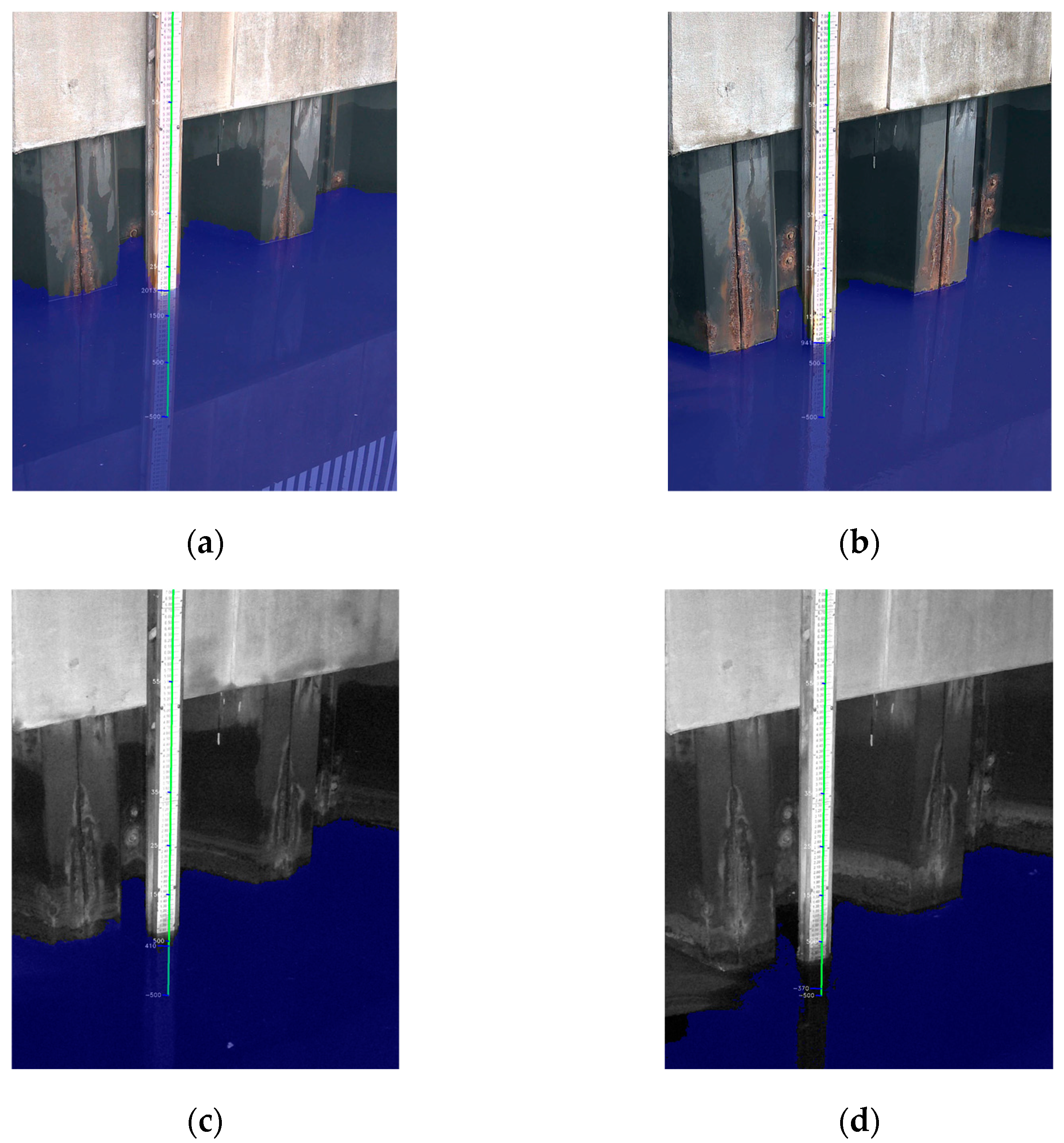
Digital gauges are defined in the configuration file as line segments, with water level breaks defined along them. Each gauge must contain one or more of such segments, and water level values are assigned to each end. Figure 2 shows an example of a gauge using one line segment, and four water level breakpoints. Calculated water level depth is also marked on the image as an example. The depth on a gauge is defined by the intersection point of the mask and the gauge line. Coordinates of the point were used to calculate the depth as a linear interpolation between depth values of two adjacent breaks. Water level was calculated for each gauge defined in the system configuration. To avoid parallax errors, we defined the gauges on permanent features, like walls or bridges, for example.
Once the algorithm finishes processing the input image, it provides the option to render an output image, with water mask and level gauge images overlaid on the original input image (blue area in Figure 2). The output metadata contain the exit status of the processing pipeline (success or error code), summarized information about the measured water levels and the location of the output image. System configuration is obtained from a configuration file which, in turn, is split into two main sections: general configuration of the system and configuration of camera-specific sections. The general section contains system settings, which are common for all cameras. The camera-specific sections concern factors that are specific to each camera, like information on water level gauges, their positions, etc. The camera section was selected based on the metadata associated with the input image, and its configuration was merged with the configuration defined by the general section, overriding the defaults. Such structure eliminates duplication of configuration sections common for all cameras (like colors, the location of the file containing model weights, etc.), while allowing for the full customization of camera-specific parameters, including the use of fine-tuned models.

2.2. USGS Datasets

In order to assess the skills of the flood detection algorithm to estimate water levels, we used data provided by the United States Geological Survey (USGS) collected within the framework of the USGS National Water Information System (https://waterdata.usgs.gov/nwis, accessed on 29 October 2023). Specifically, we used images acquired by web cameras at two selected locations in concurrence with gauge measurements of the water levels. The first site (USGS #0204295505, Figure 3a) was located at Little Neck Creek on Pinewood Road, Virginia Beach, VA (Latitude 36.859278° N, Longitude 75.984472° W, NAD83). Data were obtained for the period 15 April 2016–1 June 2023 on an hourly basis (for a total of ~62,000 h). The total number of photos after removing night values and outliers (95th percentile) was 21,456. We selected this site because the web camera was pointing at a metered water level, where the gauge was located. This could also be used to perform optimal geometric calibration which allowed for the conversion of the pixel size into water height for the digital water gauge. The second site was located at the Ottawa River near Kalida, Ohio (Latitude 40.9903287° N, Longitude 84.2266132° W). In this case, the images pointed to a bridge over a river. Also in this case, we selected the period 15 April 2016–1 June 2023, still at an hourly resolution. The total number of photos after removing night values and outliers was 24,372. We chose this image because, differently from the previous one, it showed many features (e.g., bridge, street, river, vegetation) and we wanted to test the skills of the algorithm not to detect false positives (e.g., misidentifying areas where water was not present as flooded). In this case, the water levels on the digital gauges were obtained by calibrating the relationship between pixel size and vertical resolution using the images and data collected at the minimum, maximum and middle water level values.

3. Results

3.1. Comparison between Web Camera-Estimated and Gauge Data

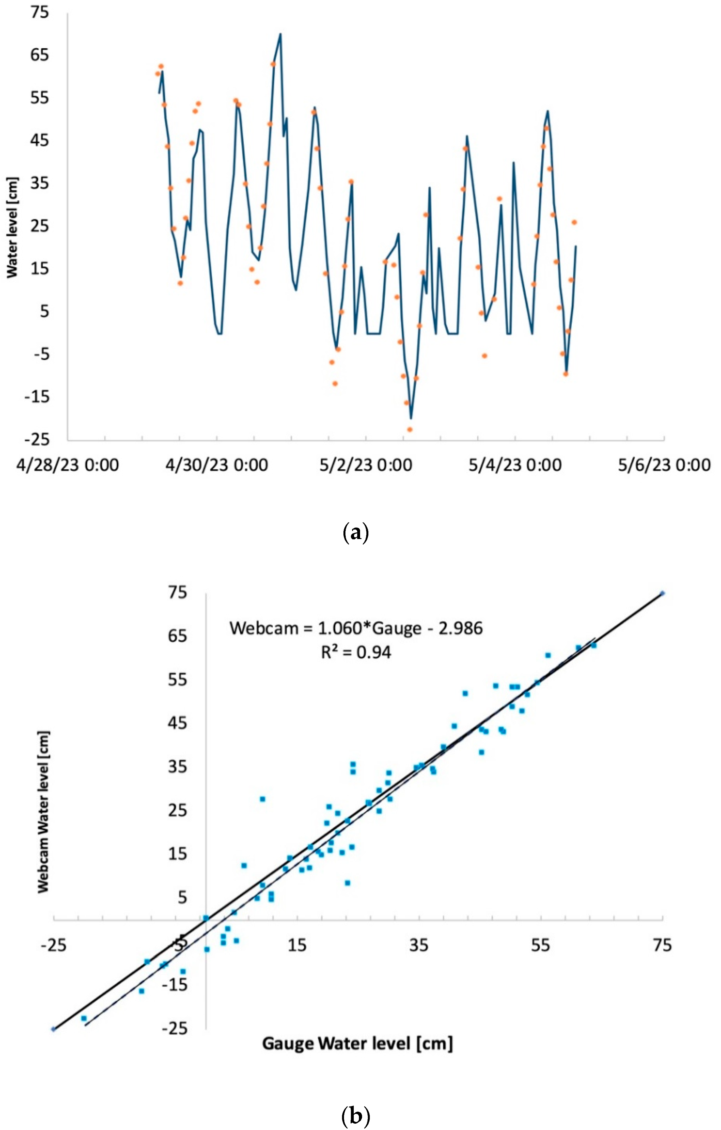
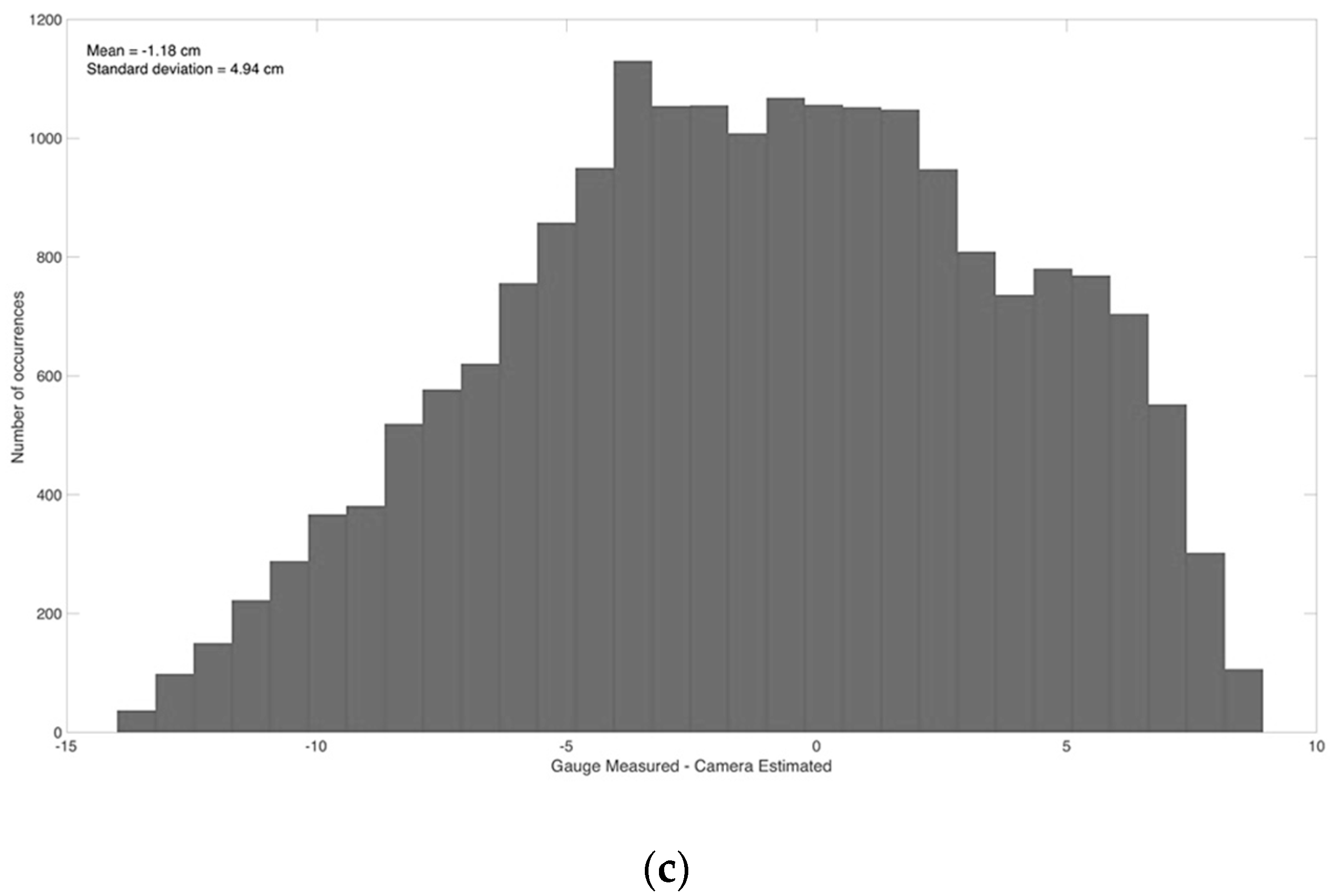
In Figure 2, we show examples of outputs of the web camera images for gauge #0204295505 for the time series of images here considered. Blue shaded regions indicate those areas where the algorithm suggests the presence of water. The digital gauge used by the algorithm to estimate the water level is also reported together with the value estimated by the algorithm for that specific frame. For visualization purposes, in Figure 3, we show the time series of water levels (in cm) estimated from tide gauge measurements (blue line) and by the machine learning algorithm using webcam images (orange squares) for the USGS gauge #0204295505 only for the period between 29 April 2023 and 5 May 2023, at hourly intervals. Gray triangles indicate nighttime acquisitions, when the images from the web camera were not used for water level detection because of the poor illumination. The skills of the algorithm to replicate gauge data are indicated by the high coefficient of determination (R2 = 0.94) and by the value of the slope (1.060) and bias (−2.98 cm, Figure 3b). When applied to the total number of images, we obtained the following statistics: R2 = 0.87, slope = 1.089 and bias = 2.44 cm. In Figure 3c, we also show the histogram of the difference between the gauge-measured and the camera-estimated water levels for all available images between 29 April 2023 and 5 May 2023. The mean and standard deviation obtained from the fitting of a normal distribution indicate a mean error of −1.18 cm and a standard deviation of 4.94 cm. Moreover, to better understand the potential role of illumination on the algorithm performance and in the absence of quantitative data concerning clouds and other information, we computed the mean and standard deviation for the data at two different periods of a day: 08:00–16:00 and 16:00–24:00. We did not consider the period 00:00–08:00 because we did not obtain camera images at night. We found that the lowest error and standard deviation were achieved for the morning period (1.12 ± 3.73 cm). The data from the afternoon period showed a mean error of −2.14 cm and a standard deviation of 5.25 cm. From Figure 2c,d, we note how, despite poor illumination conditions, the algorithm can still properly estimate water levels, though underestimation can occur. This is not unexpected, as mentioned, in view of the poor illumination conditions. Improvements in this regard could be obtained through the processing of the original image (e.g., histogram stretching) or the training of the algorithm with images acquired at night. As a reminder, indeed, the images used as the input to the algorithm were not used to train the model.
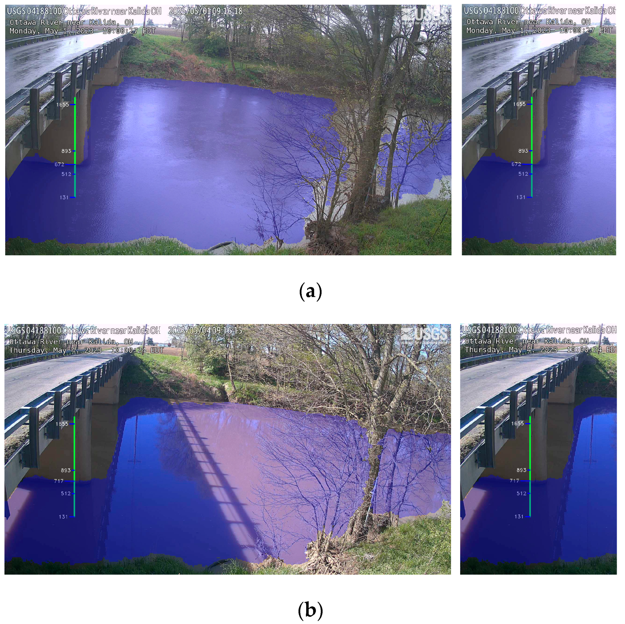
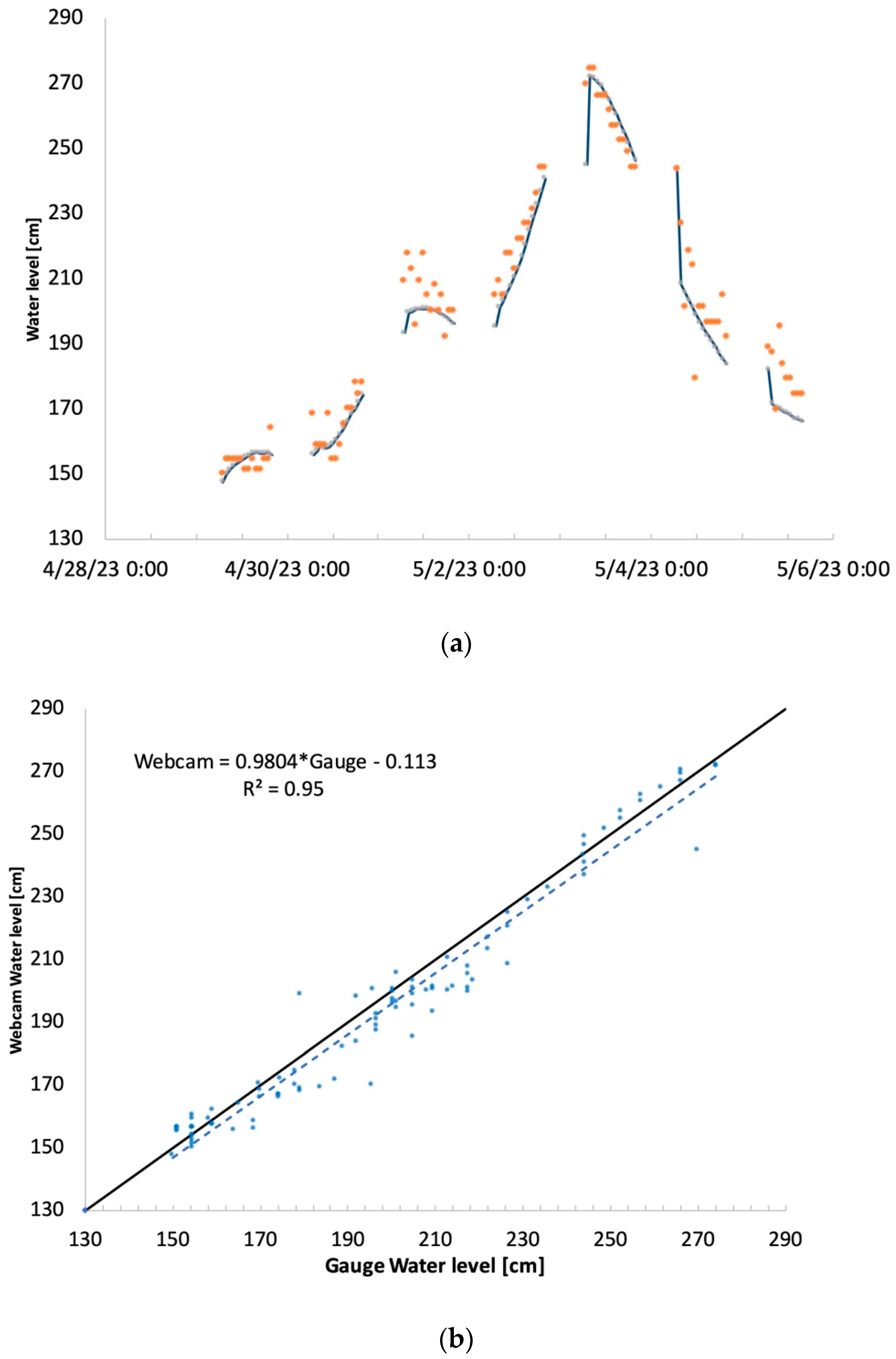
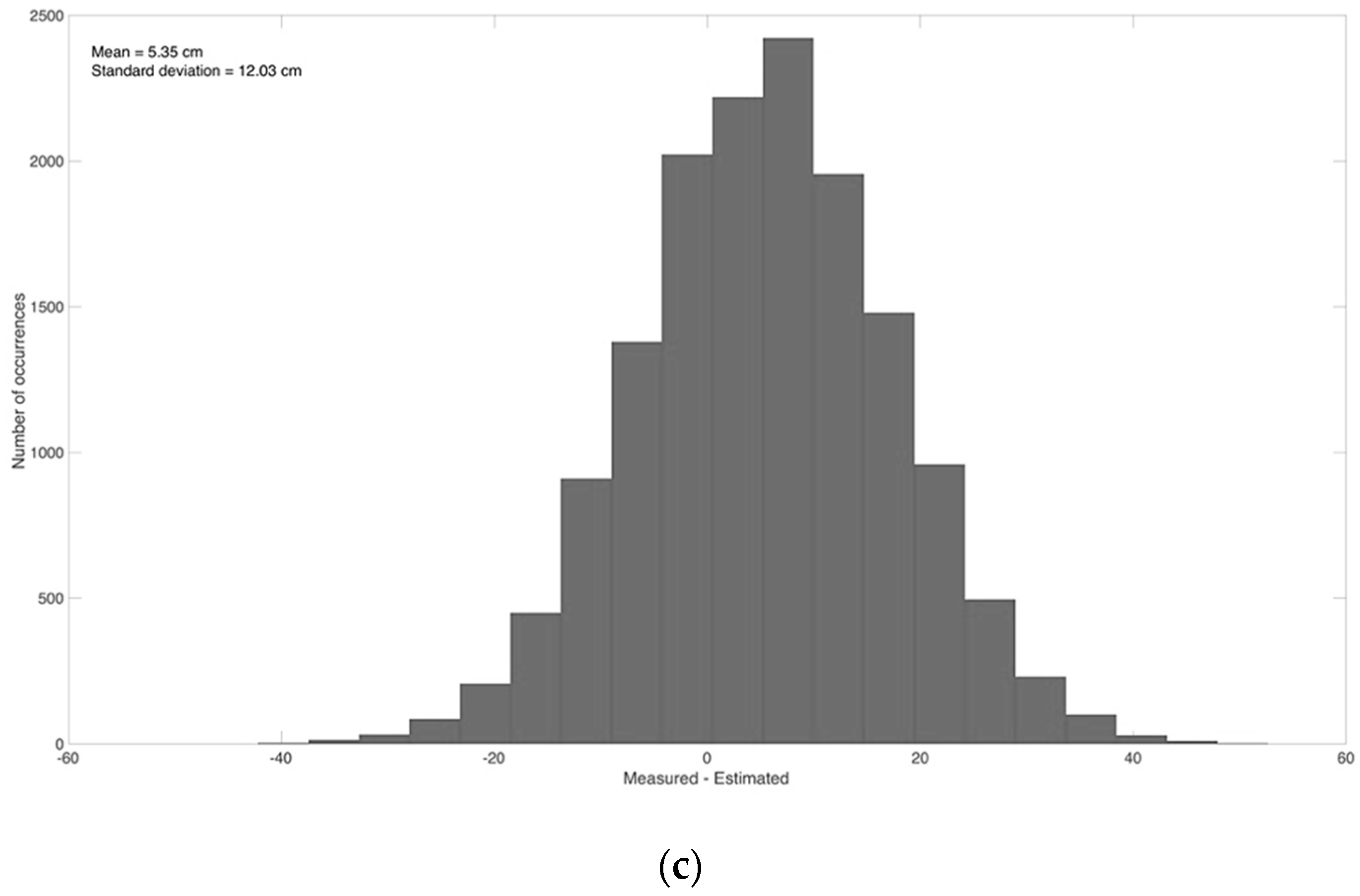
In Figure 4, we show the images obtained from the algorithm for the second selected site under two distinct illumination conditions; in the first case (Figure 4a), the image was collected under cloudy skies conditions and when rain was falling. In the other case (Figure 4b), the image was acquired under sunny conditions. Our results show that our algorithm can provide accurate estimates of water levels under both conditions. The skills of the algorithm to replicate gauge data are indicated by the high coefficient of determination (R2 = 0.95) and by the value of the slope (0.980) and bias (−0.113 cm, Figure 5b). When applied to the total number of images, we obtained the following statistics: R2 = 0.84, slope = 1.103 and bias = 3.04 cm. In the case of this gauge, images from web cameras were not available at all so it was not possible to assess the potential skills of the algorithm at night. As performed with the previous gauge, we also computed the histogram of the difference between the gauge-measured and camera-estimated water levels (Figure 5c) and found a mean difference of 5.35 cm and a standard deviation of 12.03 cm. Moreover, we computed the mean and standard deviation of the differences for the morning, afternoon and night and obtained 4.32 ± 11.76 cm (00:00–08:00), 3.78 ± 9.64 cm (08:00–16:00) and 7.28 ± 13.08 cm (16:00–24:00), respectively. These results, consistent with the ones obtained for the other gauge, indicate that the performance of the algorithm degrades during nighttime and is best in the afternoon period.

3.2. Assessment of Water Detection Skills of the Algorithm

After reporting the skills of the proposed approach to quantify water levels, we hereby discuss the potential role of the algorithm in detecting the presence of flooded regions. As already mentioned in the introduction, this can be helpful for decision and policy making, for estimates of damages or following the exposure of infrastructure to floods. For example, insurance companies might be interested in developing a system that uses images of floods collected by people or volunteers to quantitatively assess the extent and depth of water and use this to develop parametric insurance tools. Another application consists of the assessment or tuning of flood models. In this case, indeed, the data provided by our algorithm can be used to assess the skills or some of the assumptions of the algorithm. To this aim, we searched and downloaded images from the web that were collected before and during flooding over several scenes. Many of the images were available from newspapers or media outlets reporting on the specific flood event. We fed such images to the algorithm as downloaded from the web, with no alteration or manipulation. As expected, the spatial and spectral resolutions of the images can be poor. Moreover, we were only able to obtain single images rather than a sequence, hence increasing the possibility of noise or of the presence of artifacts in front of the camera (e.g., rain drops over the lens, objects covering the scene, etc.). The images used as a test offer, therefore, the most extreme, unfavorable conditions for testing the skills of the algorithm to detect water. Moreover, illumination conditions were not optimal for several images and were often different in the cases of the two images (before and after the flood) used for the testing.
We quantified the accuracy of the model in detecting the presence of water following the metrics used in [14]. For each image, we compared true positives (TPs), false positives (FPs), true negatives (TNs) and false negatives (FNs). TPs were image pixels that were correctly classified as belonging to the water region, while TNs were the numbers of pixels that were correctly classified to the non-water (background) class. For our “truth” parameter, we manually delineated the water bodies from the original images and used the corresponding masks to evaluate the outputs of the algorithm. An FP is defined as the number of pixels that did not belong to the water region but was wrongly classified as water and FNs were the pixels that were supposed to be in the water class but were incorrectly associated with the background region. We refer here to overall accuracy as the ratio between the number of pixels that were correctly identified to the total number of pixels without concerning to which class the pixels belonged.
Accuracy = (TP + TN)/(TP + TN + FP + FN)
Intersection over Union (IoU), or also known as the Jaccard coefficient, is also a standard measure used in evaluating segmentation results [4]. The IoU was computed by measuring the overlapping area between the predicted segmentation and the ground truth region.
IoU = TP/(TP + FP + FN)
The boundary F1 score (BF score) was also used to obtain detailed information on the accuracy of the segmented boundaries as the two above-mentioned metrics provided more region-based accuracies [5]. The BF score measured how close the boundary of the predicted segmentation and the ground truth segmentation was.
BF score = 2 × (Precision × Recall)/(Precision + Recall)
where precision refers to the number of correctly classified positive results divided by all positive results and recall is the number of correctly classified positive results divided by the number of samples that should have been classified as positive. We report the above-mentioned values within each caption of the images discussed below for each image for which the flood algorithm was used.
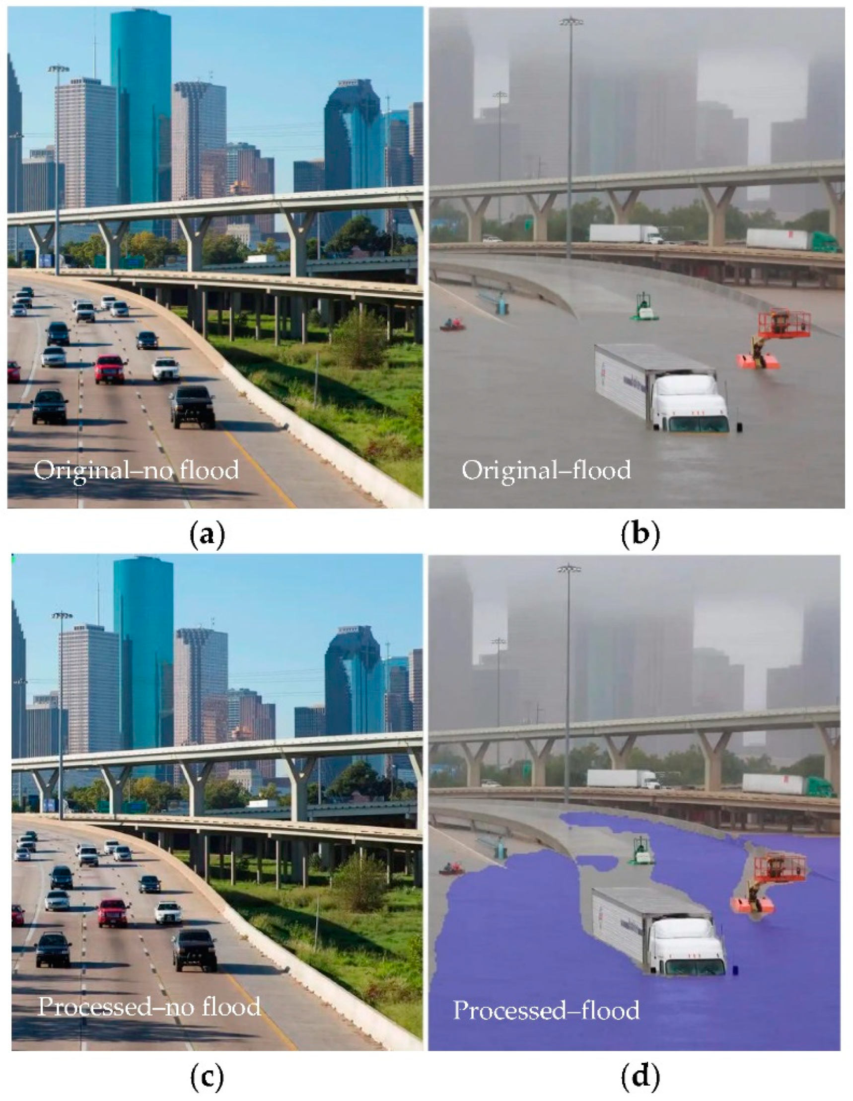
Figure 6 shows the impact of Hurricane Harvey on Houston, with the panels reporting the comparison between the original images (a,b) and those obtained as the output to the flood detection algorithm (c,d). Water is marked with the blue layer overlaying the original images. As expected, no water was detected (Figure 6c) in the image with no water (Figure 6a). Contrarily, in the case of flooding (Figure 6b), the algorithm could identify the presence of water over most of the flooded regions. The area on the mid-left of the image is not detected as flooded, likely because of the resolution of the image. In this case, the cars present in the image without flooding (Figure 6a) could be used to position a digital gauge to provide estimates of the water levels for damage assessment.
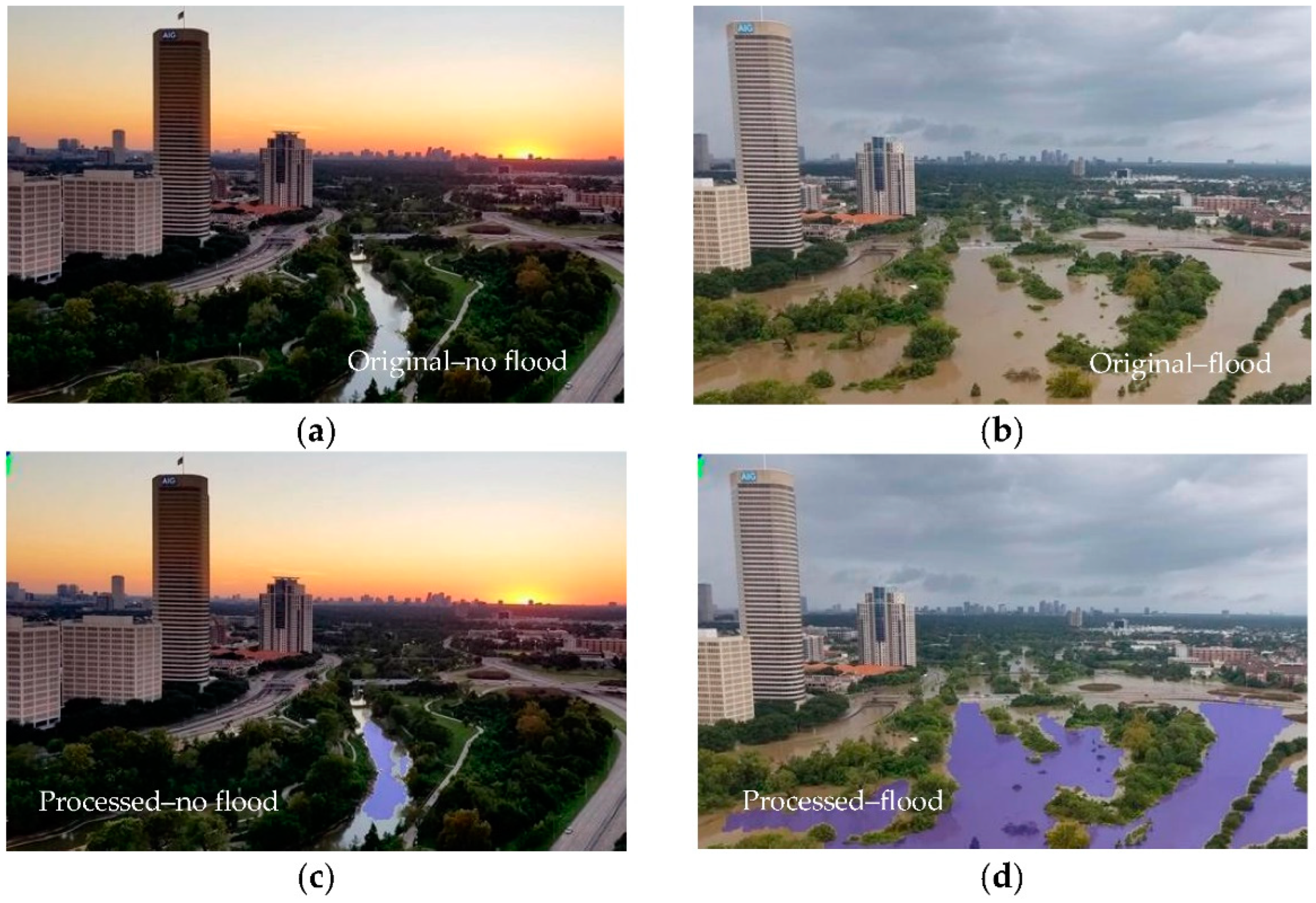
In Figure 7, we show the results obtained regarding a flood that occurred in Houston in the summer of 2018 because of Hurricane Harvey. The top left image (Figure 7a) shows the area before the flood whereas Figure 7b shows the same region after the flood occurred. Figure 7c,d show the images provided as the output by the algorithm. Despite the poor illumination of Figure 7a, the flooding algorithm properly identified the water within the river, without suggesting the presence of water where it was not. When the image containing the flooded areas was given as input to the algorithm (Figure 7b), the algorithm could properly detect flooded regions (Figure 7d), with the exception of a few patches in proximity with the pixels between the flooded region and vegetation on the right of the image.
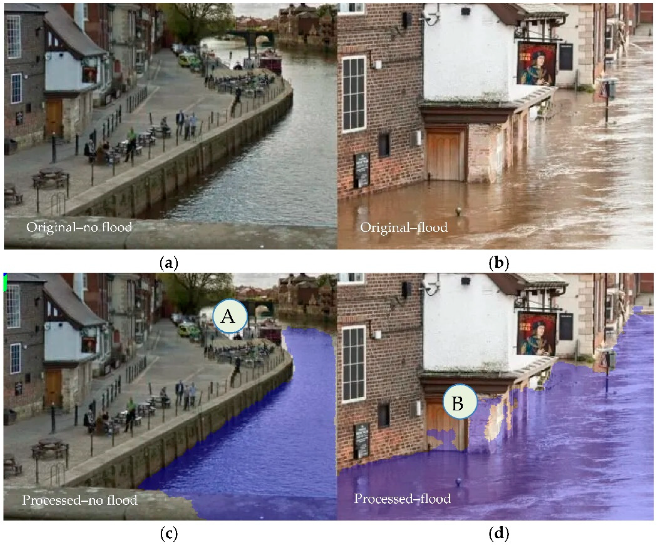
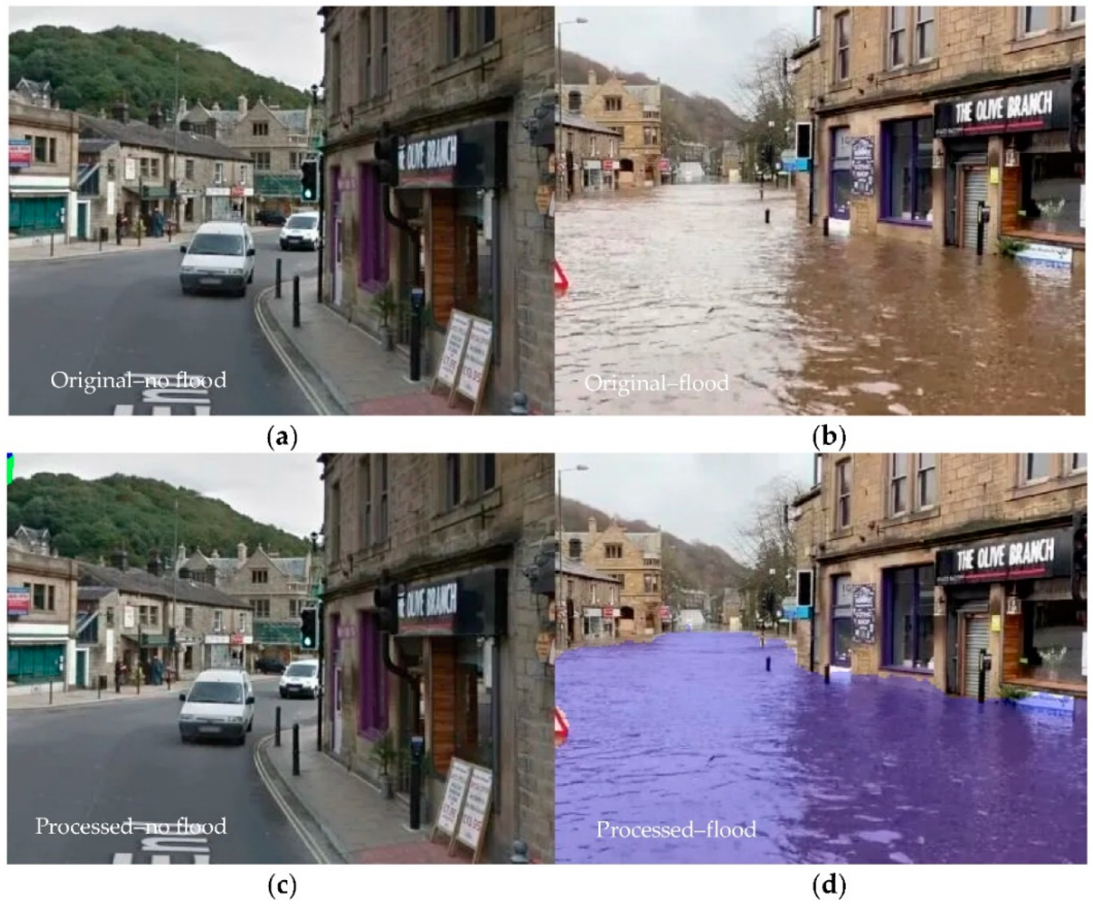
Another set of images we considered concerned flooding that occurred in the UK (York) in February 2020 (Figure 8). In Figure 8a, we show the King’s Arms, known as “the pub that floods” in York, before the flood, whereas in Figure 8b, we show an of image when flooding occurred. As in the previous cases, the algorithm properly detected the presence of the river in the close field as shown in Figure 8a. The lack of the detection of water in the far field (symbol A in Figure 8c) could be connected to the poor spatial resolution and to the distance of this area from the camera. In the case of the images containing the flooded areas (Figure 8d), we note that the algorithm could properly detect the inundated areas, though false positives existed for wet bricks and walls (see symbol B in Figure 8d). We point out that the water level for this image could be estimated once the size of the bricks was known. Similarly to Figure 8, Figure 9 shows images of West End, Hebden Bridge, West Yorkshire, on a day with no flooding (Figure 9a) versus one collected on 9 February 2020, during flooding (Figure 9b). As in the previous case, also for these images, the algorithm did not detect water when there was no flood (Figure 9c), but it was capable of properly identifying the flooded regions during the event (Figure 9d).

4. Discussion and Conclusions

We assessed the quantitative skills of a machine learning algorithm to estimate water levels within images acquired by web cameras. To this purpose, we compared the water level obtained with the machine learning algorithm with concurrent gauge measurements available for the two selected sites. Our results indicated a coefficient of determination of R2 of 0.94–0.95, a maximum absolute bias of −2.98 cm and a slope ranging between 0.980 and 1.06 in the two cases here considered, highlighting the skills of the algorithm used to estimate water levels from the web cameras images. We note again that the model was not trained with any of the images provided to the algorithm, pointing to the potential general nature of the machine learning algorithm here used [12]. Our analysis of the histogram of the differences between gauge-measured and camera-estimated water levels indicated a mean difference of −1.18 cm (gauge #0204295505) and 5.35 cm (gauge #04188100). Moreover, when sub-setting the data in the morning and afternoon observations, we found that the best (worst) performance was obtained in the case of the observations collected in the morning (at night). This suggests that illumination might be a driving factor of the deterioration of the algorithm’s performance. However, we cannot at this stage rule out other factors and we plan to assess this aspect in our future work.
Our analysis of the performance of the algorithm to detect water from images obtained from the web and containing scenes of areas before and after a flooding event showed that the accuracy of the algorithm exceeded ~90%, with the Intersection over Union (IoU) and the boundary F1 score (both used to assess the output of segmentation analysis) exceeding ~80% (IoU) and 70% (BF1).
Improvements can, of course, always be made via the re-training of the model using specific, tailored datasets, such as those collected at nighttime or during extreme conditions in specific locations where the algorithm is applied, for example. Nevertheless, our results here indicate that the proposed algorithm can be used for several applications “as is”, such as in parametric insurance, post-disaster estimates and model validation, catalyzing our skills to monitor flooding via the merging of the ubiquitous nature of web camera images with the robustness of the machine learning model results and the agile architecture built around the model, which allow for its deployment in any environment in a seamless way.

Author Contributions

Conceptualization, M.T.; methodology, M.T.; software, M.T. and J.R.; formal analysis, M.T.; writing—review and editing, M.T. All authors have read and agreed to the published version of the manuscript.

Funding

This research was funded by Liguria Digitale SPA-AD_LD_2022_215.

Data Availability Statement

All images used in this paper are available at the links reported in the text. The software is available upon request. Inquiries should be sent to [email protected].

Acknowledgments

The authors thank the anonymous reviewers and editors for their suggestions.

Conflicts of Interest

The authors declare no conflict of interest. The funders had no role in the design of the study; in the collection, analyses or interpretation of data; in the writing of the manuscript; or in the decision to publish the results.

References

  1. Colgan, C.S.; Beck, M.W.; Narayan, S. Financing Natural Infrastructure for Coastal Flood Damage Reduction; Lloyd’s Tercentenary Research Foundation: London, UK, 2017; Available online: https://www.middlebury.edu/institute/sites/www.middlebury.edu.institute/files/2018-07/6.13.17.LLYODS.Financing%20Natural%20Infrastructure%201.JUN_.2017_Lo%20Res.pdf (accessed on 9 May 2023).
  2. Xafoulis, N.; Kontos, Y.; Farsirotou, E.; Kotsopoulos, S.; Perifanos, K.; Alamanis, N.; Dedousis, D.; Katsifarakis, K. Evaluation of Various Resolution DEMs in Flood Risk Assessment and Practical Rules for Flood Mapping in Data-Scarce Geospatial Areas: A Case Study in Thessaly, Greece. Hydrology 2023, 10, 91. [Google Scholar] [CrossRef]
  3. Billah, M.; Islam, A.S.; Bin Mamoon, W.; Rahman, M.R. Random forest classifications for landuse mapping to assess rapid flood damage using Sentinel-1 and Sentinel-2 data. Remote Sens. Appl. Soc. Environ. 2023, 30, 100947. [Google Scholar] [CrossRef]
  4. Hamidi, E.; Peter, B.G.; Munoz, D.F.; Moftakhari, H.; Moradkhani, H. Fast Flood Extent Monitoring with SAR Change Detection Using Google Earth Engine. IEEE Trans. Geosci. Remote Sens. 2023, 61, 1–19. [Google Scholar] [CrossRef]
  5. Refice, A.; D’Addabbo, A.; Capolongo, D. (Eds.) Methods, Techniques and Sensors for Precision Flood Monitoring Through Remote Sensing. In Flood Monitoring through Remote Sensing; Springer Remote Sensing/Photogrammetry; Springer International Publishing: Cham, Switzerland, 2018; pp. 1–25. [Google Scholar] [CrossRef]
  6. Tedesco, M.; McAlpine, S.; Porter, J.R. Exposure of real estate properties to the 2018 Hurricane Florence flooding. Nat. Hazards Earth Syst. Sci. 2020, 20, 907–920. [Google Scholar] [CrossRef]
  7. Giustarini, L.; Hostache, R.; Matgen, P.; Schumann, G.J.; Bates, P.D.; Mason, D.C. A change detection approach to flood mapping in urban areas using TerraSAR-X. IEEE Trans. Geosci. Remote Sens. 2013, 51, 2417–2430. [Google Scholar] [CrossRef]
  8. Windheuser, L.; Karanjit, R.; Pally, R.; Samadi, S.; Hubig, N.C. An End-To-End Flood Stage Prediction System Using Deep Neural Networks. Earth Space Sci. 2023, 10, e2022EA002385. [Google Scholar] [CrossRef]
  9. Le, Q.-C.; Le, M.-Q.; Tran, M.-K.; Le, N.-Q.; Tran, M.-T. FL-Former: Flood Level Estimation with Vision Transformer for Images from Cameras in Urban Areas. In Multimedia Modeling; Dang-Nguyen, D.-T., Gurrin, C., Larson, M., Smeaton, A.F., Rudinac, S., Dao, M.-S., Trattner, C., Chen, P., Eds.; Lecture Notes in Computer Science; Springer International Publishing: Cham, Switzerland, 2023; Volume 13833, pp. 447–459. [Google Scholar] [CrossRef]
  10. Donratanapat, N.; Samadi, S.; Vidal, J.; Tabas, S.S. A national scale big data analytics pipeline to assess the potential impacts of flooding on critical infrastructures and communities. Environ. Model. Softw. 2020, 133, 104828. [Google Scholar] [CrossRef]
  11. Liang, Y.; Li, X.; Tsai, B.; Chen, Q.; Jafari, N. V-FloodNet: A video segmentation system for urban flood detection and quantification. Environ. Model. Softw. 2023, 160, 105586. [Google Scholar] [CrossRef]
  12. Vandaele, R.; Dance, S.L.; Ojha, V. Deep learning for automated river-level monitoring through river-camera images: An approach based on water segmentation and transfer learning. Hydrol. Earth Syst. Sci. 2021, 25, 4435–4453. [Google Scholar] [CrossRef]
  13. Chen, L.C.; Papandreou, G.; Schroff, F.; Adam, H. Rethinking Atrous Convolution for Semantic Image Segmentation. arXiv 2017, arXiv:1706.05587. [Google Scholar] [CrossRef]
  14. Lopez-Fuentes, L.; Rossi, C.; Skinnemoen, H. River segmentation for flood monitoring. In Proceedings of the 2017 IEEE International Conference on Big Data (Big Data), Boston, MA, USA, 11–14 December 2017; pp. 3746–3749. [Google Scholar] [CrossRef]
  15. Muhadi, N.A.; Abdullah, A.F.; Bejo, S.K.; Mahadi, M.R.; Mijic, A. Deep Learning Semantic Segmentation for Water Level Estimation Using Surveillance Camera. Appl. Sci. 2021, 11, 9691. [Google Scholar] [CrossRef]
  16. Zhang, Z.; Zhou, Y.; Liu, H.; Zhang, L.; Wang, H. Visual Measurement of Water Level under Complex Illumination Conditions. Sensors 2019, 19, 4141. [Google Scholar] [CrossRef]
  17. Qiao, G.; Yang, M.; Wang, H. A Water Level Measurement Approach Based on YOLOv5s. Sensors 2022, 22, 3714. [Google Scholar] [CrossRef] [PubMed]
  18. Eltner, A.; Elias, M.; Sardemann, H.; Spieler, D. Automatic Image-Based Water Stage Measurement for Long-Term Observations in Ungauged Catchments. Water Resour. Res. 2018, 54, 10362–10371. [Google Scholar] [CrossRef]
  19. Muste, M.; Ho, H.-C.; Kim, D. Considerations on direct stream flow measurements using video imagery: Outlook and research needs. J. Hydro-Environ. Res. 2011, 5, 289–300. [Google Scholar] [CrossRef]
  20. Lo, S.-W.; Wu, J.-H.; Lin, F.-P.; Hsu, C.-H. Visual Sensing for Urban Flood Monitoring. Sensors 2015, 15, 20006–20029. [Google Scholar] [CrossRef]
  21. Schoener, G. Time-Lapse Photography: Low-Cost, Low-Tech Alternative for Monitoring Flow Depth. J. Hydrol. Eng. 2018, 23, 06017007. [Google Scholar] [CrossRef]
  22. Lin, Y.-T.; Lin, Y.-C.; Han, J.-Y. Automatic water-level detection using single-camera images with varied poses. Measurement 2018, 127, 167–174. [Google Scholar] [CrossRef]
  23. Zhen, Z.; Yang, Z.; Yuchou, L.; Youjie, Y.; Xurui, L. IP Camera-Based LSPIV System for On-Line Monitoring of River Flow. In Proceedings of the 2017 IEEE 13th International Conference on Electronic Measurement & Instruments (ICEMI), Yangzhou, China, 20–22 October 2017; pp. 357–363. [Google Scholar] [CrossRef]
  24. Xu, Z.; Feng, J.; Zhang, Z.; Duan, C. Water Level Estimation Based on Image of Staff Gauge in Smart City. In Proceedings of the 2018 IEEE SmartWorld, Ubiquitous Intelligence & Computing, Advanced & Trusted Computing, Scalable Computing & Communications, Cloud & Big Data Computing, Internet of People and Smart City Innovation (SmartWorld/SCALCOM/UIC/ATC/CBDCom/IOP/SCI), Guangzhou, China, 8–12 October 2018; pp. 1341–1345. [Google Scholar] [CrossRef]
  25. Leduc, P.; Ashmore, P.; Sjogren, D. Technical note: Stage and water width measurement of a mountain stream using a simple time-lapse camera. Hydrol. Earth Syst. Sci. 2018, 22, 1–11. [Google Scholar] [CrossRef]
  26. Tsubaki, R.; Fujita, I.; Tsutsumi, S. Measurement of the flood discharge of a small-sized river using an existing digital video recording system. J. Hydro-Environ. Res. 2011, 5, 313–321. [Google Scholar] [CrossRef]
  27. Creutin, J.; Muste, M.; Bradley, A.; Kim, S.; Kruger, A. River gauging using PIV techniques: A proof of concept experiment on the Iowa River. J. Hydrol. 2003, 277, 182–194. [Google Scholar] [CrossRef]
  28. Ran, Q.-H.; Li, W.; Liao, Q.; Tang, H.-L.; Wang, M.-Y. Application of an automated LSPIV system in a mountainous stream for continuous flood flow measurements: LSPIV for Mountainous Flood Monitoring. Hydrol. Process. 2016, 30, 3014–3029. [Google Scholar] [CrossRef]
  29. Stumpf, A.; Augereau, E.; Delacourt, C.; Bonnier, J. Photogrammetric discharge monitoring of small tropical mountain rivers: A case study at Rivière des Pluies, Réunion Island. Water Resour. Res. 2016, 52, 4550–4570. [Google Scholar] [CrossRef]
  30. Chen, C.; Fu, R.; Ai, X.; Huang, C.; Cong, L.; Li, X.; Jiang, J.; Pei, Q. An Integrated Method for River Water Level Recognition from Surveillance Images Using Convolution Neural Networks. Remote Sens. 2022, 14, 6023. [Google Scholar] [CrossRef]
  31. Dou, G.; Chen, R.; Han, C.; Liu, Z.; Liu, J. Research on Water-Level Recognition Method Based on Image Processing and Convolutional Neural Networks. Water 2022, 14, 1890. [Google Scholar] [CrossRef]
  32. Krähenbühl, P.; Koltun, V. Efficient Inference in Fully Connected CRFs with Gaussian Edge Potentials. arXiv 2012, arXiv:1210.5644. [Google Scholar] [CrossRef]
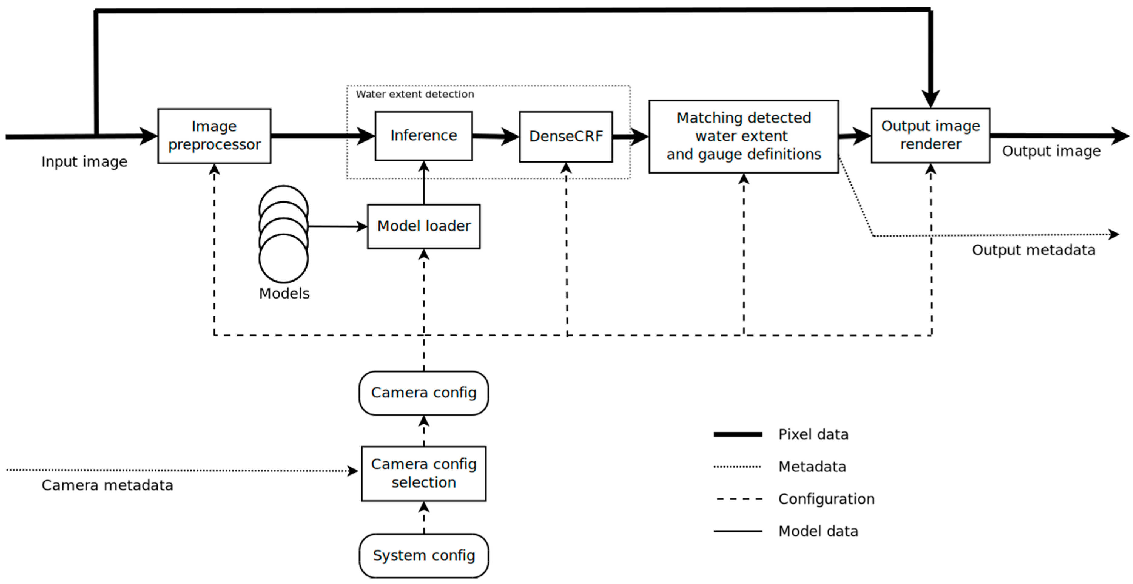
Figure 1. Architecture of the algorithm adopted in this study.
Geohazards 04 00025 g001
Figure 2. Examples of outputs of the web camera images for gauge #0204295505 collected on (a) 29 April 2023, 6:30 AM, (b) 30 April 2023, 3:30 PM, (c) 1 May 2023, 21:30 and (d) 2 May 2023, 00:25. Blue shaded regions indicate where the algorithm identified the presence of water. The digital gauge used by the algorithm to estimate the water level is also reported together with the value estimated by the algorithm. Original image resolution: 300 dpi. Original image size: 700 × 700.
Geohazards 04 00025 g002
Figure 3. (a) Time series of water levels (in cm) estimated from tide gauge measurements (blue line) and the algorithm using webcam images (orange squares) for the USGS gauge #0204295505 between 29 April 2023 and 5 May 2023. (b) Scatterplot of the water level (in cm) obtained from gauge (x-axis) and webcam images (y-axis) for the same period as (a). The 1:1 line is also reported as a continuous black line. The shaded line represents the linear fitting with its equation reported in the inset of (b) together with the coefficient of determination (R2). (c) Histogram of the difference between the gauge-measured and the camera-estimated water levels for all available images between 29 April 2023 and 5 May 2023. The mean and standard deviation of the normal distribution fitting the data are also reported within the plot.
Geohazards 04 00025 g003aGeohazards 04 00025 g003b
Figure 4. Examples of outputs of the web camera images for gauge #04188100. Blue shaded regions indicate where the algorithm identified the presence of water. The digital gauge used by the algorithm to estimate the water level is also reported together with the value estimated by the algorithm. (a) the image was collected under cloudy skies conditions and when rain was falling; (b), the image was acquired under sunny conditions. Original image resolution: 300 dpi. Original image size: 1200 × 700.
Geohazards 04 00025 g004
Figure 5. (a) Time series of water levels (in cm) estimated from tide gauge measurements (blue line) and the algorithm using webcam images (orange squares) for the USGS gauge #04188100 between 29 April 2023 and 5 May 2023. (b) Scatterplot of the water level (in cm) obtained from gauge (x-axis) and webcam images (y-axis) for the same period as (a). The 1:1 line is also reported as a continuous black line. The shaded line represents the linear fitting with its equation reported in the inset of (b) together with the coefficient of determination (R2). (c) Histogram of the difference between the gauge-measured and the camera-estimated water levels for all available images between 29 April 2023 and 5 May 2023. The mean and standard deviation of the normal distribution fitting the data are also reported within the plot.
Geohazards 04 00025 g005aGeohazards 04 00025 g005b
Figure 6. Comparison between the original images (a,b) and those obtained as the output to the flood detection algorithm (c,d). Water is marked with the blue layer overlaying the original images. Image source adapted from https://www.theguardian.com/us-news/2017/aug/29/before-and-after-images-show-how-hurricane-harvey-swamped-houston, accessed on 29 October 2023. Original image resolution: 72 dpi. Original image size: 1000 × 1200. (d) Accuracy: 93.5%; IoU = 89.3%; BF = 73.2%.
Geohazards 04 00025 g006
Figure 7. Comparison between the original images (a,b) and those obtained as the output to the flood detection algorithm (c,d). Water is marked with the blue layer overlaying the original images. Original images obtained ftom https://www.nbc4i.com/news/before-and-after-photos-illustrate-massive-houston-flooding/, accessed on 29 October 2023. Original image resolution: 72 dpi. Original image size: 864 × 486. (c) Accuracy: 94.1%; IoU = 86.1%; BF = 74.8%.; (d) Accuracy: 90.1%; IoU = 84.3%; BF = 69.2%.
Geohazards 04 00025 g007
Figure 8. Comparison between the original images (a,b) and those obtained as the output to the flood detection algorithm (c,d). Water is marked with the blue layer overlaying the original images. Original images obtained from https://www.huffingtonpost.co.uk/entry/before-and-after-pictures-february-uk-floods_uk_5e539ebbc5b6b82aa655ab2b, accessed on 29 October 2023. Original image resolution: 72 dpi. Original image size: 410 × 312. (c) Accuracy: 98.2%; IoU = 90%; BF = 78.2%; (d) Accuracy: 96.1%; IoU = 81.6%; BF = 70.9%.
Geohazards 04 00025 g008
Figure 9. Comparison between the original images (a,b) and those obtained as the output to the flood detection algorithm (c,d). Water is marked with the blue layer overlaying the original images. for West End, Hebden Bridge, West Yorkshire. Images adapted from https://www.huffingtonpost.co.uk/entry/before-and-after-pictures-february-uk-floods_uk_5e539ebbc5b6b82aa655ab2, accessed on 29 October 2023. Original image resolution: 72 dpi. Original image size: 410 × 312. (d) Accuracy: 98.2%; IoU = 86.7%; BF = 77.4%.
Geohazards 04 00025 g009
Disclaimer/Publisher’s Note: The statements, opinions and data contained in all publications are solely those of the individual author(s) and contributor(s) and not of MDPI and/or the editor(s). MDPI and/or the editor(s) disclaim responsibility for any injury to people or property resulting from any ideas, methods, instructions or products referred to in the content.