Technical Note

Effect of Base Conditions in One-Dimensional Numerical Simulation of Seismic Site Response: A Technical Note for Best Practice

1
CNR-IGAG, Istituto di Geologia Ambientale e Geoingegneria, Area della Ricerca di Roma 1, via Salaria km 29,300, Monterotondo Stazione, 00015 Roma, Italy
2
Presidenza del Consiglio dei Ministri—Dipartimento della Protezione Civile (DPC), via Vitorchiano 2, 00189 Roma, Italy
*
Author to whom correspondence should be addressed.
GeoHazards 2021, 2(4), 430-441; https://doi.org/10.3390/geohazards2040024
Submission received: 26 September 2021 / Revised: 14 December 2021 / Accepted: 16 December 2021 / Published: 18 December 2021

Abstract

:
The effects induced by the choice of numerical base conditions for evaluating local seismic response are investigated in this technical note, aiming to provide guidelines for professional applications. A numerical modelling of the seismic site response is presented, assuming a one-dimensional scheme. At first, with reference to the case of a homogeneous soil layer overlying a half-space, two different types of numerical base conditions, named rigid and elastic, were adopted to analyse the seismic site response. Then, geological setting, physical and mechanical properties were selected from Italian case studies. In detail, the following stratigraphic successions were considered: shallow layer 1 (shear wave velocity, VS, equal to 400 m/s), layer 2 (VS equal to 600 m/s) and layer 3 (VS equal to 800 m/s). In addition, real signals were retrieved from the web site of the Italian accelerometric strong motion network. Rigid and elastic base conditions were adopted to estimate the ground motion modifications of the reference signals. The results are presented in terms of amplification factors (i.e., ratio of integral quantities referred to free-field and reference response spectra) and are compared between the adopted numerical models.

1. Introduction

Local seismic site response (LSSR) analysis allows the estimation of the ground motion induced by the propagation of surface or body waves. Seismic microzonation studies are generally based on one-dimensional LSSR schemes, as we have observed during our more than 10-years activity on-field in Italy. This technical note provides a reference for professional applications.
Numerical or analytical approaches require a definition of the local subsoil conditions and of the so-called reference site [1,2,3,4]. Local subsoil conditions are defined in terms of mechanical and geometrical properties [5,6,7,8,9]: geological subsoil models are characterized by the geometry of buried morphologies and topographical surfaces, combined with the profile of shear wave velocity with the depth [VS(z)], unit weight of soil (γt), plasticity index (PI), relative density (DR), nonlinear curves referring to the decay of secant shear stiffness [GS(γ)/G0] and the increment of damping ratio [D(γ)] with shear strain (γ). On the other hand, the reference site is required to define the input motion (i.e., the time history of acceleration or velocity or displacement or stress) for the LSSR. In addition, the base condition of the numerical model depends on the mechanical and geometrical properties of the site of interest and of the reference site [10,11,12,13,14]. In detail, referring to the one-dimensional numerical modelling of LSSR, the so called rigid and elastic base conditions should be adopted depending on the site where the known motion has been recorded. The rigid base condition can be adopted (i) if the input motion is recorded at the base of the deposit of interest (for example, see point B in Figure 1), disregarding the impedance contrast between such a deposit and the underlying strata, or (ii) if the input motion is recorded at the outcrop of a stiff material (see point O in Figure 1) and the impedance contrast (briefly, the ratio between the stiffness of the half-space and of the deposit) is theoretically equal to infinite. Truthfully, if the input motion is recorded at the ground surface of the outcropping half-space (i.e., point O in Figure 1), referring to most Italian diffuse case studies, the so-called elastic base condition should be adopted since the impedance contrast between the half-space material and the deposit of interest is in the range 1.5–6 [9]: hence, lower than infinite. In this context, it is worth noting that the terms rigid and elastic refer to the numerical base conditions, rather than to the stiffness of the soil.
With reference to the homogeneous deposit (i.e., physical and mechanical properties constant with depth), typical case studies were selected from the Italian database for seismic microzonation (https://www.webms.it/ (accessed on 1 February 2021)), where site data and seismic microzonation studies (about 4000) have been collected since 2008. A brief comparison between the results obtained by means of numerical modelling of LSSR based on the rigid and elastic base conditions is presented. In detail, referring to a single input motion, the effect of the impedance contrast was investigated. Furthermore, it is worth noting that the Italian urban sites are generally characterised by a three-layered lithostratigraphic succession, assumed as follows (from top to bottom) [8,15]: layer 1 with shear wave velocity, VS, in the order of 400 m/s; layer 2 with VS in the range 400–800 m/s; layer 3 with VS higher than 800 m/s. For sake of brevity, the VS succession 400–600–800 m/s was considered to perform LSSR analyses. Moreover, referring to the selected heterogeneous site condition, a set of 132 signals were retrieved from the Italian Accelerometric Archive, briefly ITACA (accessible at http://itaca.mi.ingv.it/ItacaNet_30/#/home (accessed on 1 February 2021)), and were adopted as input motions considering both rigid and elastic base numerical conditions. Hence, with reference to the heterogeneous case study, the correlation between base conditions and ground motion was considered by varying the input motion.
The results are presented in terms of pseudo-acceleration response spectra and amplification factors (Afs), quantified according to Equation (1):
AF T 1 - T 2 = T 1 T 2 Sa o dT T 1 T 2 Sa i dT
where, Sa is the pseudo-spectral acceleration, the subscripts o and i refer to the free-field and reference signal, respectively, and T is the period. T1 and T2 are referred to the period intervals considered in the integral quantities, that are, in this study, 0.1–0.5 s, 0.4–0.8 s, and 0.7–1.1 s, in agreement with other researchers [16,17,18,19]. AFs based on rigid and elastic base numerical conditions are compared aiming to verify the effect of the base condition on the forecasting of ground motion. Overall, the main issues were: (i) finding the value of the impedance contrast which provided comparable results based on rigid and elastic base numerical conditions, and (ii) evaluating the difference between rigid and elastic results varying the input motion.

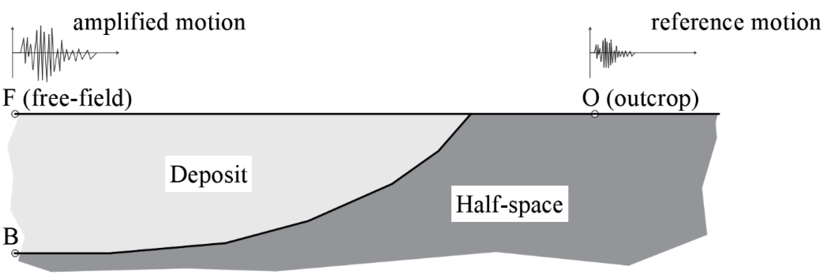
2. Numerical Modelling of Seismic Site Response

The numerical modelling of the seismic site response is presented here with reference to homogeneous case studies (i.e., a homogeneous deposit overlying a half-space) and heterogeneous one-dimensional case studies (i.e., a succession characterised by VS increasing with depth overlying a half-space). Moreover, the correlation between the results and the adopted base conditions (i.e., rigid and elastic base of the numerical model) is provided. In detail, referring to the homogeneous case studies, only one reference motion was retrieved from the ITACA database, since the key issue to be enlightened was the effect of rigid and elastic base numerical conditions, in the presence of impedance contrasts in the range of 1.5–82. Furthermore, for two realistic case studies (i.e., deposits characterised by vertical lithostratigraphic heterogeneity) a set of 132 reference motions were selected to gauge the effect of the input motion variation on the numerical results.

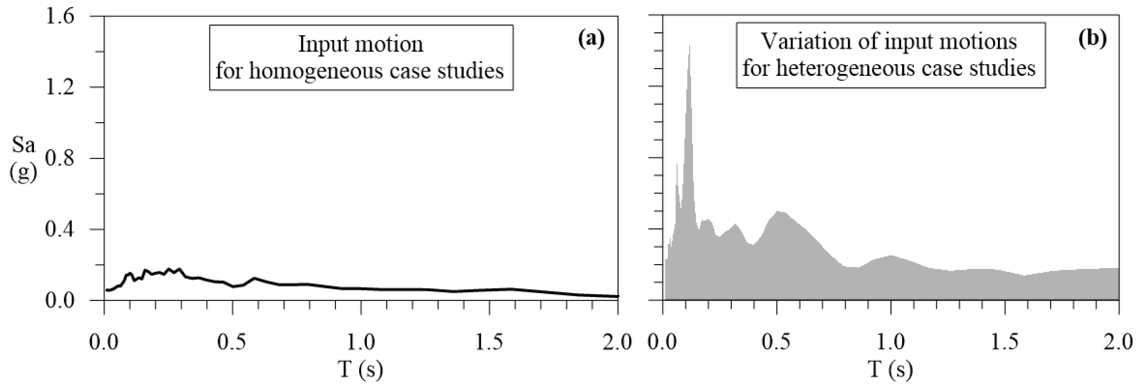
2.1. Homogenous Deposit

The numerical modelling of the seismic site response with reference to homogeneous one-dimensional case studies is presented in this section. The linear visco-elastic mechanical behaviour was assumed for sake of convenience. With reference to the deposit, the following physical and mechanical parameters were considered VS = 300, 400, 600, 800 m/s, D = 2% and γt = 18 kN/m3. With reference to the half-space, the following physical and mechanical parameters were considered VS = 800, 2000, 3000 m/s, D = 1% and γt = 22 kN/m3. In addition, an unrealistic half-space VS equal to 20,000 m/s was selected to gauge the ground motion response in the presence of a very stiff half-space, adopting the elastic base numerical condition. As a matter of fact, it is expected that the results based on elastic base numerical condition and VS = 20,000 m/s for the half-space should agree with the results obtained by means of rigid base numerical condition. In addition, the thickness of the deposit, H, was assumed equal to 15 and 100 m.
The response spectra of the input motion, shown in Figure 2a, refers to the Irpinia earthquake, Mw = 6.9 (where Mw is the moment magnitude), occurred on 23rd November 1980 in Italy, as recorded by the Auletta station of the Italian accelerometric network [20,21]. This station is placed at the flat ground surface of outcropping polygenic conglomerate, characterized by the harmonic mean of the shear wave velocity in the upper 30 m, VS30, equal to 1018 m/s. In addition, no peak value of the horizontal to vertical spectral ratio (HVSR) was reported in the station monography (available at http://itaca.mi.ingv.it/ItacaNet_30/#/station/IT/ALT (accessed on 1 February 2021)). Hence, Auletta station was considered a reference station. The numerical simulations were performed by means of the code STRATA [22]. Like SHAKE [23,24], STRATA adopt the linear equivalent approach in the frequency domain. It is worth noting that the selected reference motion is characterised by spectral acceleration, Sa, greater than 0 g for periods in the range 0–2.0 s. Hence, bearing in mind that the fundamental frequencies of selected homogeneous deposits are those listed in Table 1, the selected reference signal was useful to provide amplification phenomena referring to the whole range of periods of interest.
For the sake of brevity, Figure 3 only shows the response spectra obtained at the ground surface of the deposit (i.e., free field) and refers to VS equal to 400 m/s. It is worth noting that the numerical rigid base condition forecast is generally higher than that based on the numerical elastic base condition. The differences between numerical rigid and elastic base results are limited to periods lower than 0.4 s for H = 15 m since no amplification phenomena occurs for such a shallow deposit at higher periods. On the other hand, with reference to H = 100 m, the rigid base results are the highest for periods lower than 2.0 s; in fact, the fundamental frequency f0 of such a deposit is equal to 1 Hz (see Table 1). Hence, as expected, the numerical base condition plays a crucial role in the LSSR analyses.
To enlighten the difference between the forecasts obtained by means of numerical rigid and elastic base conditions, the error was quantified according to the Equation (2).
ε AF = AF r i g i d AF e l a s t i c AF e l a s t i c 100
It is important to underline that εAF greater than 0 refers to the case studies where the numerical rigid model overestimates the result obtained by means of the numerical elastic model, whereas εAF lower than 0 refers to the case studies where the numerical rigid model underestimates the result obtained by means of the numerical elastic model.
In addition, the impedance contrast, I, between the deposit and the underlying half-space was quantified according to the Equation:
1 = 1 ρ deposit · G deposit ρ half-space · G half-space
where ρ is the mass density, G is the secant shear modulus, and the subscript “half-space” refers to the base of the numerical model. It should be noted that the higher the Ghalf-space with respect to the Gdeposit, the higher the I. Hence, the εAF is plotted as a function of I for each examined case study, as shown in Figure 4 and Figure 5 with reference to deposit thickness equal to 15 and 100 m, respectively. In general, it is worth noting that: (i) the higher the I, the lower the overestimation of the rigid base forecast; (ii) the overestimation of the rigid base forecast is lower than 20% for I higher than 30; (iii) the deeper the deposit the higher the periods characterized by the overestimation of the rigid base forecast; (iv) with reference to the deposit thickness equal to 100 m and deposit VS lower than 400 m/s, the higher the period the higher the overestimation of the rigid base forecast.

2.2. Heterogenous Case Studies

Real site conditions are more complex than those presented in the previous section. For instance, the VS increases with depth, and GS and D depend on the intensity of the ground shaking (i.e., shear strain induced by the seismic waves). In this context, results referred to two heterogeneous case studies are here presented. Figure 6 shows the selected VS profiles and GS(γ)/G0 and D(γ) curves [25]. In the same figure, soil material characterised by VS equal to 400, 600, and 800 m/s are named Unit 1, 2, and 3, respectively. Moreover, for that material characterized by VS, at least equal to 800 m/s, a linear visco-elastic mechanical behaviour was considered by assuming GS(γ)/G0 = 1 and D(γ) = 1%. With reference to Units 1, 2, and 3, the γt was assumed equal to 18, 19, and 22 kN/m3, respectively.
A set of 132 real acceleration time histories were retrieved from the ITACA database [20], referring to stations on outcropped soils characterized by VS30 at least equal to 800 m/s and flat topography; Figure 2b shows the pseudo-acceleration response spectra selected as input motions for the numerical LSSR analyses. The peak ground acceleration is in the range 0.05–0.22 g, as representative of the Italian seismic hazard with reference to a return period equal to 475 years, and the peak values of the pseudo-spectral acceleration refer to periods lower than 0.8 s.
Figure 7 shows the distributions of the error εAF, determined according to the Equation (2), referring to the two selected heterogeneous site profiles (see Figure 6a). As mentioned with reference to the homogeneous case studies, the rigid base condition overestimates the AF obtained by means of numerical simulation, carried out adopting the elastic base condition. In general, with reference to the heterogeneous site profile 1, the higher the range of the period the lower the mean value of the distribution of εAF. Conversely, with reference to the heterogeneous site profile 2, the higher the range of the period the higher the mean value of the εAF distribution. In detail, referring to the heterogeneous site profile 1 and to the period ranges 0.1–0.5 s, 0.4–0.8 s, and 0.7–1.1 s, the mean values of the εAF distributions are equal to 192%, 44%, and 36%, respectively. Moreover, referring to the heterogeneous site profile 2 and to the same period ranges, the mean values of the εAF distributions are equal to 112%, 65%, and 160%, respectively.
Finally, Figure 8 shows the profiles of the maximum shear strain, γmax, induced by the seismic waves’ propagation. The γmax at the base of the numerical models refer to the rigid base condition being higher than the γmax at the base of the numerical models, referring to the elastic base condition, as expected. In fact, the outcrop motion is applied at the base of the numerical model, as in the case of the rigid base condition, whereas only the upcoming seismic waves included in the outcrop motion are applied at the base of the numerical model in the case of the elastic base condition.

3. Conclusions

Seismic microzonation studies are generally based on one-dimensional local seismic site response schemes, as we have observed during our more than 10-years activity on-field (scientific webinars, workshops for technicians, and so on); regarding the Italian experience see, for example, https://govrisv.cnr.it/ (accessed on 30 June 2021) and https://www.webms.it/ (accessed on 30 June 2021). In addition, real site conditions cannot be easily imported in numerical code for seismic site response analysis. Hence, we decided to provide this technical note on the effect of the numerical base condition in a one-dimensional scheme on the ground motion modification phenomenon.
To highlight how rigid and elastic base conditions of the numerical model affect the local seismic site response, numerical modelling was performed, adopting the one-dimensional scheme. The well-known code, STRATA, by Kottke et al. [21] was adopted. The code is based on the equivalent linear approach in the frequency domain. With reference to homogeneous and heterogeneous site profiles, both the numerical rigid and elastic base conditions were selected to perform local seismic site response analyses. The results were presented in terms of errors quantified by comparing the amplification factors referring to the rigid and elastic base numerical models. In general, it was observed that:
-
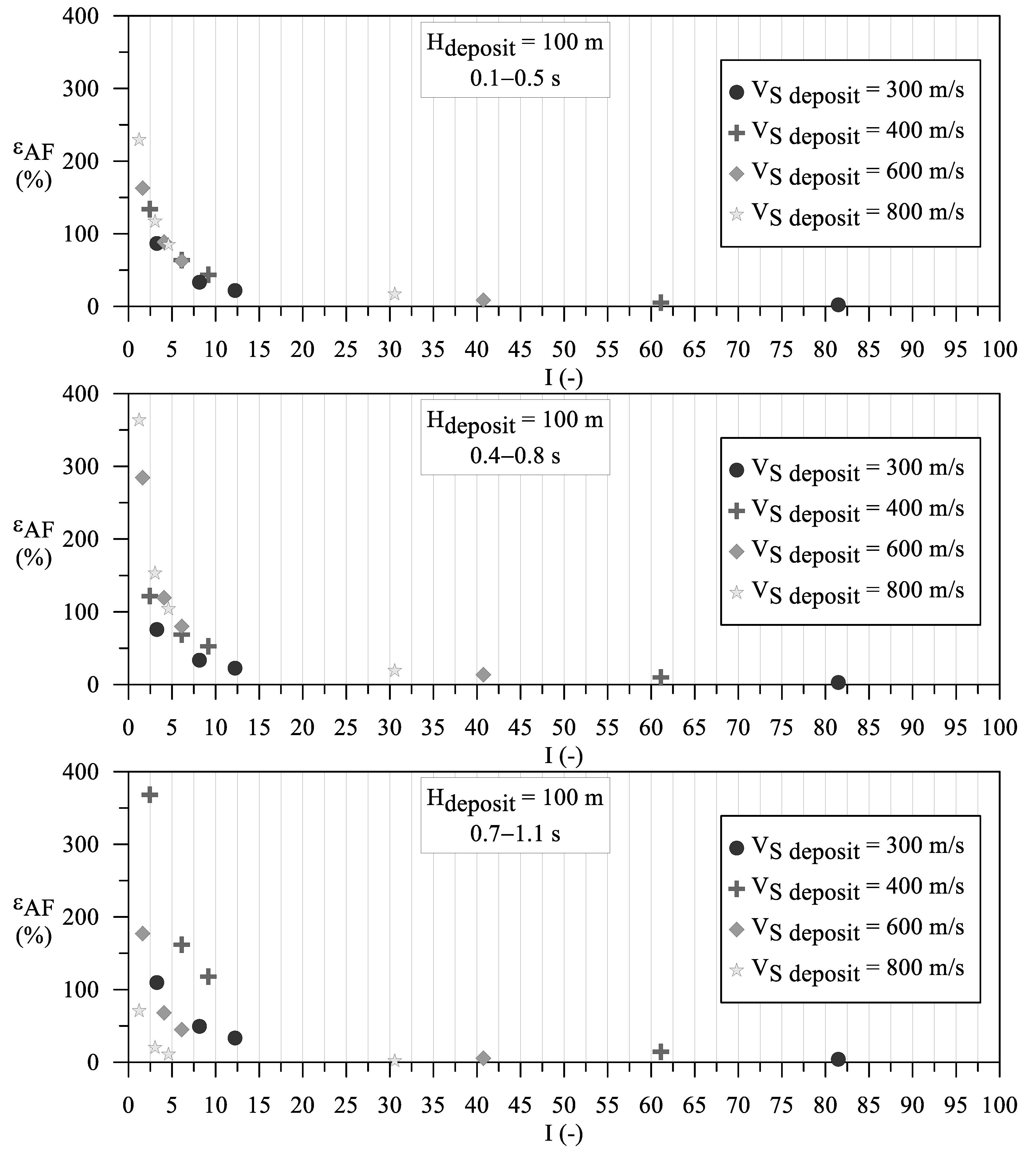
The higher the impedance ratio between the deposit and the half-space (i.e., the base of the numerical model) the lower the error. In detail, the rigid and elastic base results agree for impedance contrasts higher than 30;
-
Referring to shallow deposits (thickness lower than 30 m), the higher the range of periods of interest, the lower the overestimation of the rigid base models, with respect to the elastic base ones;
-
Referring to deep deposits (thickness higher than 100 m), the higher the range of periods of interest, the higher the overestimation of the rigid base models with respect to the elastic base ones.
As a final recommendation, the elastic base condition should be preferred to the rigid base condition when dealing with site conditions comparable to those adopted in this work (one-dimensional scheme, shear wave velocity of the deposit constant or increasing with depth, thickness of the deposit lower than 100 m and impedance contrast between deposit and half-space lower than 30). Further research could be focused on the comparison between rigid and elastic base conditions with reference to very high intensity earthquakes (peak ground acceleration higher than 0.3 g), to more realistic site profiles (including shear wave velocity inversion), and to two or three-dimensional geometries.

Author Contributions

Conceptualization, G.F., G.N. and F.M.; methodology, G.F. and G.N.; formal analysis, G.F.; resources, F.M.; data curation, G.F., G.N. and F.M.; writing—original draft preparation, G.F. and G.N.; writing—review and editing, G.F., G.N., F.M., A.M., G.A., E.P. and M.M.; visualization, G.F.; supervision, G.F., G.N., F.M., A.M., G.A., E.P. and M.M.; project administration, G.N., F.M., E.P. and M.M.; funding acquisition, M.M. All authors have read and agreed to the published version of the manuscript.

Funding

This research was supported by the Italian Department for Civil Protection of the Presidency of Council of Ministers within the “Contratto concernente l’affidamento di servizi per il programma per il supporto al rafforzamento della Governance in materia di riduzione del rischio sismico e vulcanico ai fini di protezione civile nell’ambito del PON Governance e Capacità Istituzionale 2014–2020—CIG6980737E65”.

Institutional Review Board Statement

Not applicable.

Informed Consent Statement

Not applicable.

Data Availability Statement

The data presented in this study are available on request from the corresponding author.

Acknowledgments

Authors gratefully acknowledge two anonymous reviewers, the Assistant Editor David Hu and the Editorial Board for helping to improve the quality of the manuscript. Authors gratefully acknowledge the support provided by the Managing Editor Haley Shi. Authors would like to thank F. Bramerini, S. Castenetto, A. Gorini, and D. Spina (Italian Department for Civil Protection) for the useful discussions.

Conflicts of Interest

The authors declare no conflict of interest.

References

  1. Kramer, S. Geotechnical Earthquake Engineering; Prentice Hall: Upper Saddle River, NJ, USA, 1996; ISBN 9780133749434. [Google Scholar]
  2. Moczo, P.; Kristek, J.; Bard, P.Y.; Stripajová, S.; Hollender, F.; Chovanová, Z.; Kristeková, M.; Sicilia, D. Key structural parameters affecting earthquake ground motion in 2D and 3D sedimentary structures. Bull. Earthq. Eng. 2018, 16, 2421–2450. [Google Scholar] [CrossRef] [Green Version]
  3. Makra, K.; Chávez-García, F.J.; Raptakis, D.; Pitilakis, K. Parametric analysis of the seismic response of a 2D sedimentary valley: Implications for code implementations of complex site effects. Soil Dyn. Earthq. Eng. 2005, 25, 303–315. [Google Scholar] [CrossRef]
  4. Falcone, G.; Acunzo, G.; Mendicelli, A.; Mori, F.; Naso, G.; Peronace, E.; Porchia, A.; Romagnoli, G.; Tarquini, E.; Moscatelli, M. Seismic amplification maps of Italy based on site-specific microzonation dataset and one-dimensional numerical approach. Eng. Geol. 2021, 289, 106170. [Google Scholar] [CrossRef]
  5. Rathje, E.M.; Kottke, A.R.; Trent, W.L. Influence of input motion and site property variabilities on seismic site response analysis. J. Geotech. Geoenviron. Eng. 2010, 136, 607–619. [Google Scholar] [CrossRef]
  6. Guzel, Y.; Rouainia, M.; Elia, G. Effect of soil variability on nonlinear site response predictions: Application to the Lotung site. Comput. Geotech. 2020, 121, 103444. [Google Scholar] [CrossRef]
  7. Régnier, J.; Bonilla, L.; Bard, P.; Bertrand, E.; Hollender, F.; Kawase, H.; Sicilia, D.; Arduino, P.; Amorosi, A.; Asimaki, D.; et al. PRENOLIN: International Benchmark on 1D Nonlinear Site-Response Analysis—Validation Phase Exercise. Bull. Seismol. Soc. Am. 2018, 108, 876–900. [Google Scholar] [CrossRef]
  8. Falcone, G.; Romagnoli, G.; Naso, G.; Mori, F.; Peronace, E.; Moscatelli, M. Effect of bedrock stiffness and thickness on numerical simulation of seismic site response. Italian case studies. Soil Dyn. Earthq. Eng. 2020, 139, 106361. [Google Scholar] [CrossRef]
  9. Talukder, M.K.; Rosset, P.; Chouinard, L. Reduction of Bias and Uncertainty in Regional Seismic Site Amplification Factors for Seismic Hazard and Risk Analysis. GeoHazards 2021, 2, 277–301. [Google Scholar] [CrossRef]
  10. Callisto, L.; Rampello, S.; Viggiani, G.M.B. Soil–structure interaction for the seismic design of the Messina Strait Bridge. Soil Dyn. Earthq. Eng. 2013, 52, 103–115. [Google Scholar] [CrossRef] [Green Version]
  11. Falcone, G.; Boldini, D.; Amorosi, A. Site response analysis of an urban area: A multi-dimensional and non-linear approach. Soil Dyn. Earthq. Eng. 2018, 109, 33–45. [Google Scholar] [CrossRef]
  12. Falcone, G.; Boldini, D.; Martelli, L.; Amorosi, A. Quantifying local seismic amplification from regional charts and site specific numerical analyses: A case study. Bull. Earthq. Eng. 2020, 18, 77–107. [Google Scholar] [CrossRef]
  13. Régnier, J.; Bonilla, L.; Bard, P.; Bertrand, E.; Hollender, F.; Kawase, H.; Sicilia, D.; Arduino, P.; Amorosi, A.; Asimaki, D.; et al. International Benchmark on Numerical Simulations for 1D, Nonlinear Site Response (PRENOLIN): Verification Phase Based on Canonical Cases. Bull. Seismol. Soc. Am. 2016, 106, 2112–2135. [Google Scholar] [CrossRef]
  14. Mejia, L.H.; Dawson, E.M. Earthquake deconvolution for FLAC. In Proceedings of the 4th International FLAC Symposium on Numerical Modeling in Geomechanics, Madrid, Spain, 29–31 May 2006; Itasca Consulting Group: Minneapolis, MN, USA, 2006. [Google Scholar]
  15. DPC. Dipartimento della Protezione Civile Commissione Tecnica per il Supporto E Monitoraggio Degli Studi di Microzonazione Sismica (ex art.5, OPCM3907/10), (2018)—WebMs; WebCLE. A cura di: Maria Sole Benigni, Fabrizio Bramerini, Gianluca Carbone, Sergio Castenetto, Gian Paolo Cavinato, Monia Coltella, Margherita Giuffrè, Massimiliano Moscatelli, Giuseppe Naso, Andrea Pietrosante, Francesco Stigliano. 2018; Available online: www.webms.it (accessed on 01 February 2021).
  16. Gaudiosi, I.; Simionato, M.; Mancini, M.; Cavinato, G.P.; Coltella, M.; Razzano, R.; Sirianni, P.; Vignaroli, G.; Moscatelli, M. Evaluation of site effects at Amatrice (central Italy) after the 24th August 2016, Mw 6.0 earthquake. Soil Dyn. Earthq. Eng. 2021, 144, 106699. [Google Scholar] [CrossRef]
  17. Giallini, S.; Pizzi, A.; Pagliaroli, A.; Moscatelli, M.; Vignaroli, G.; Sirianni, P.; Mancini, M.; Laurenzano, G. Evaluation of complex site effects through experimental methods and numerical modelling: The case history of Arquata del Tronto, central Italy. Eng. Geol. 2020, 272, 105646. [Google Scholar] [CrossRef]
  18. Moscatelli, M.; Albarello, D.; Scarascia Mugnozza, G.; Dolce, M. The Italian approach to seismic microzonation. Bull. Earthq. Eng. 2020, 18, 5425–5440. [Google Scholar] [CrossRef]
  19. Falcone, G.; Mendicelli, A.; Mori, F.; Fabozzi, S.; Moscatelli, M.; Occhipinti, G.; Peronace, E. A simplified analysis of the total seismic hazard in Italy. Eng. Geol. 2020, 267, 105511. [Google Scholar] [CrossRef]
  20. ITACA. ITalian ACcelerometric Archive. Retrieved April, 2020.. 2019. Available online: http://itaca.mi.ingv.it/ItacaNet_30/#/home (accessed on 01 February 2021).
  21. Luzi, L.; Pacor, F.; Puglia, R. Italian Accelerometric Archive v3.0. Istituto Nazionale di Geofisica e Vulcanologia; Dipartimento della Protezione Civile Nazionale: Rome, Italy, 2001. [Google Scholar] [CrossRef]
  22. Kottke, A.; Wang, X.; Rathje, E.M. Technical Manual for Strata. Rep. No. 2008/10; Pacific Earthquake Engineering Research Center: Berkeley, CA, USA, 2013. [Google Scholar]
  23. Schnabel, P.B.; Lysmer, J.; Seed, H.B. Shake: A Computer Program for Earthquake Response Analysis of Horizontally-Layered sites; Technical Report EERC-72/12; Earthquake Engineering Research Centre, University of California: Berkeley, CA, USA, 1972. [Google Scholar]
  24. Idriss, M.; Sun, J.I. SHAKE91: A Computer Program for Conducting Equivalent Linear Seismic Response Analyses of Horizontally Layered Soil Deposits; Centre for Geotechnical Modelling, Department of Civil and Environmental Engineering, University of California: Davis, CA, USA, 1992. [Google Scholar]
  25. Darendeli, M.B. Development of a New Family of Normalized Modulus Reduction and Material Damping Curves; University of Texas: Austin, TX, USA, 2001. [Google Scholar]
Figure 1. Simplified seismic site response scheme.
Geohazards 02 00024 g001
Figure 2. Response spectra of the reference motions in pseudo-spectral acceleration referring to: (a) homogeneous case studies and (b) heterogeneous case studies.
Geohazards 02 00024 g002
Figure 3. Response spectra in pseudo-acceleration obtained by means of rigid and elastic base conditions, with reference to linear visco-elastic materials and cover deposit thickness H equal to 15 m (left side) and 100 m (right side).
Geohazards 02 00024 g003
Figure 4. Error in the estimation of AFs quantified according to the Equation (2), with reference to cover deposit thickness equal to 15 m and linear visco-elastic materials. In detail, assuming VS = 20,000 m/s for the half-space, the impedance contrast results equal to 81.5, 61.1, 40.7, and 30.6 with reference to the deposit VS equal to 300, 400, 600, and 800 m/s, respectively.
Geohazards 02 00024 g004
Figure 5. Error in the estimation of AFs quantified according to Equation (2), with reference to cover deposit thickness equal to 100 m and linear visco-elastic materials. In detail, assuming VS = 20,000 m/s for the half-space, the impedance contrast results equal to 81.5, 61.1, 40.7, and 30.6 with reference to deposit VS equal to 300, 400, 600, and 800 m/s, respectively.
Geohazards 02 00024 g005
Figure 6. Mechanical parameters for the heterogeneous case study: (a) VS-z profiles, (b) GS(γ)/G0 and D(γ) curves (briefly, NL curves), and (c) soil units–depth range–NL curves association.
Geohazards 02 00024 g006
Figure 7. Distribution of εAF referring to the heterogenous site profile 1 (Hdeposit = 30 m) and to the heterogenous site profile 2 (Hdeposit = 120 m).
Geohazards 02 00024 g007
Figure 8. Profiles of maximum shear strain, γmax, with depth referring to the heterogenous site profile 1 (Hdeposit = 30 m) and to the heterogenous site profile 2 (Hdeposit = 120 m).
Geohazards 02 00024 g008
Table 1. Theoretical fundamental frequencies and periods related to the selected homogeneous case studies.
HVSf0T0
(m)(m/s)(Hz)(s)
153005.000.20
154006.670.15
1560010.000.10
1580013.330.08
1003000.751.33
1004001.001.00
1006001.500.67
1008002.000.50
Publisher’s Note: MDPI stays neutral with regard to jurisdictional claims in published maps and institutional affiliations.

