Research on Obtaining Pepper Phenotypic Parameters Based on Improved YOLOX Algorithm

Abstract

Pepper is a vital crop with extensive agricultural and industrial applications. Accurate phenotypic measurement, including plant height and stem diameter, is essential for assessing yield and quality, yet manual measurement is time-consuming and labor-intensive. This study proposes a deep learning-based phenotypic measurement method for peppers. A Pepper-mini dataset was constructed using offline augmentation. To address challenges in multi-plant growth environments, an improved YOLOX-tiny detection model incorporating a CA attention mechanism was developed, achieving a mAP of 95.16%. A detection box filtering method based on Euclidean distance was introduced to identify target plants. Further processing using HSV threshold segmentation, morphological operations, and connected component denoising enabled accurate region selection. Measurement algorithms were then applied, yielding high correlations with true values: $R^2$ = 0.973 for plant height and $R^2$ = 0.842 for stem diameter, with average errors of 0.443 cm and 0.0765 mm, respectively. This approach demonstrates a robust and efficient solution for automated phenotypic analysis in pepper cultivation.

1. Introduction

Pepper has garnered significant attention in modern agriculture [1,2,3]. With the increasing and mature application of technology in agriculture, the yield of pepper has been substantially improved [4,5,6]. To study the growth status of pepper, real-time measurements of various phenotypic parameters such as plant height and stem diameter at different stages of growth are essential. However, obtaining crop phenotypic parameters typically relies on traditional manual methods [7,8], requiring researchers to personally measure and collect samples in the field [9,10]. Due to the long growth cycle of crops, researchers cannot continuously monitor them in real time, especially during critical growth stages [11]. If the growth conditions are not detected during these important periods, it may result in missing or incomplete phenotypic information [12]. As a consequence, multiple repeated experiments become necessary, leading to a heavy workload, low efficiency, and reduced accuracy [13]. Moreover, the measurement results are susceptible to human factors, resulting in poor readability of the results and subsequently affecting the phenotypic and growth assessment of the crops [14].

In 1987, Mayer et al. [15] were the first to apply image processing techniques to measure phenotypic parameters such as leaf area, stem diameter, and leaf inclination in crops. In 1996, Casady et al. [16] used machine vision technology to process images of two different rice varieties at the pixel level, obtaining plant height, width, area, and other characteristic parameters with good correlation compared to manual measurements. Wang et al. [17] utilized computer vision technology to classify the plant diseases and pests of 22 kinds of plants. Chen et al. [18] developed a high-throughput image framework for phenotypic analysis, using this framework to conduct experiments on various barley varieties’ responses to drought conditions. Mora et al. [19] employed a two-step image segmentation method in different color spaces to eliminate non-foliage interference on leaf area index. They validated the effectiveness of this method by detecting cherry tree canopies. Zhu et al. [20] proposed a high-throughput detection method for tomato plant phenotypes based on multi-view 3D structure reconstruction. Their experimental results demonstrated its good performance in measuring phenotypic parameters such as plant height and canopy width. Although traditional image processing techniques have made notable progress in the field of crop phenotyping, they often rely on machine learning or other algorithmic approaches that require handcrafted feature design and substantial domain expertise [21,22]. This reliance significantly limits their applicability and scalability in plant phenotyping applications [7].

In recent years, the rapid development of Convolutional Neural Network (CNN) technology based on deep learning has surpassed traditional image processing and computer vision methods in terms of accuracy and effectiveness [23,24,25,26,27,28,29]. CNNs achieve higher-level semantic representations by progressively coupling lower-level features, making them highly advantageous for research and applications in crop phenotyping. Numerous researchers have achieved significant breakthroughs in various areas of crop phenotyping using deep learning-based CNNs [30,31]. Some notable applications include disease identification in fruits and vegetables [32,33], the identification of intact maize kernels [34], and wheat ear counting [35]. These accomplishments demonstrate the immense potential of CNNs in advancing crop research and agricultural practices. Baweja et al. [36] combined a target detection network model in deep learning with a image segmentation model to detect the stalk width of corn, sugarcane, and other crops. The experimental results confirmed that the measurement rate and the accuracy of the results are far superior to those of traditional manual methods. Deep learning has also been applied to estimate the quantity of large-area crops in drone images by Bending et al. [37]. Similarly, Li et al. [38] proposed a peanut yield estimation method based on RT-DETR, which was deployed on an unmanned ground vehicle (UGV) for field validation. In flower image phenotyping, Yuan et al. [39] proposed a framework based on transfer learning and a bilinear CNN for chrysanthemum image classification with high accuracy. Similarly, Wang et al. [17] proposed a high-accuracy plant disease and pest classification framework based on a Vision Transformer (ViT) and Masked Autoencoder (MAE). Adar et al. [40] proposed a length measurement technique based on object detection, interest point recognition, and 3D measurement. The experimental results showed an error control within $10\%$, indicating its potential to replace manual measurement to some extent. Chen et al. [41] addressed the issue of irreproducibility and low detection accuracy in existing internal plant structure phenotyping methods. They proposed an attention-enhanced multiscale segmentation model (MCC-Net) for the non-destructive segmentation and detection of rice seedling stems, which proved to be effective. Li et al. [42] proposed a real-time detection and segmentation method for in-field blueberry phenotyping, based on SAM and YOLOv8n. Previous studies have successfully implemented automated measurement tasks across various crops such as maize, sugarcane, wheat, and tomato. For instance, Baweja et al. [36] proposed the StalkNet model for detecting stem width in maize and sugarcane; Li et al. [38] employed RT-DETR for peanut yield estimation and deployed the system on a ground unmanned platform; Yuan et al. [39] utilized transfer learning and a bilinear CNN architecture for chrysanthemum image classification. Additionally, Wang et al. [43] developed a high-precision crop disease and pest identification model based on a Vision Transformer. These studies demonstrate the widespread application of deep learning methods in crop phenotypic trait recognition. However, there is still a lack of accurate phenotypic measurement systems specifically designed for pepper crops under complex growth environments. This demonstrates the significant application potential of deep learning technologies in the domain of plant phenotyping.

In summary, while previous research has explored the measurement of other plant phenotypic parameters, there has not been a systematic study on measuring pepper phenotypic parameters using deep learning. Therefore, this paper adopts a deep learning approach and systematically measures pepper phenotypic parameters such as plant height and stem diameter. The main contributions of this paper are the following:

• Construction of the Pepper-mini dataset. This study verifies the conversion relationship of unit pixels at different distances for the detection system. It utilizes offline data augmentation to construct the Pepper-mini dataset from the collected pepper image dataset, which can be openly used.
• Optimization of YOLOX-tiny object detection algorithm using the CA attention mechanism. This study enhances the network’s feature extraction capability for peppers, improving the overall object detection performance. It identifies target plants based on the Euclidean distance-based object detection box filtering rule. This study utilizes image processing operations such as threshold segmentation, morphological changes, and connected area denoising in the HSV color space to extract binary images of the processed target plants. Finally, this study applies plant height and stem diameter measurement algorithms to achieve precise measurements of the target plants.
• Proposal and application of a novel plant height and stem diameter measurement algorithm, which to some extent can replace manual measurements.

2. Materials and Methods

2.1. Construction of the Pepper-Mini Dataset

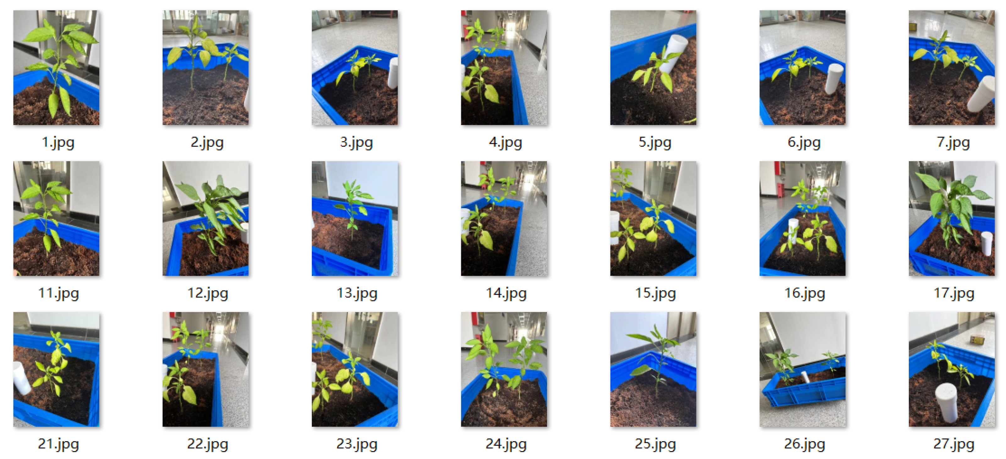
2.1.1. Data Collection

The Pepper-mini dataset was derived from our self-built aquaponic system and the Qingxi organic farm in Shangzhuang Town, Haidian District, Beijing (116.185° E, 40.137° N). The images were captured using a Huawei Nova 8 Pro smartphone equipped with a 64MP high-resolution camera. By continuously collecting growth data over three growth cycles, we obtained a total of 210 pepper plant images. These images cover different growth stages, ranging from seedling to fruiting, providing diverse information for the model to learn richer features and improve its generalization capability. Some sample images are shown in Figure 1.

2.1.2. Data Augmentation

In order to enrich the diversity of the data, improve the reliability and accuracy of the network model detection, and avoid overfitting, it is necessary to expand the dataset. This study adopted an offline approach for expansion, using methods such as rotation, flipping, random cropping, brightness adjustment, and noise addition. The initial dataset was increased from 210 to 1235 images after data expansion and manual screening. The expanded dataset from the initial one consists of the following three parts:

• Dataset with rotation, flipping, and random cropping. The initial dataset was rotated by 10° and 350°, and horizontally flipped.
• Dataset with brightness adjustment. The initial dataset was transformed from the RGB color space to the HSV color space, and then the brightness (Value, V) channel was increased by 10% and decreased by 10%.
• Dataset with added noise. The initial dataset was processed with salt-and-pepper noise and Gaussian noise.

2.1.3. Data Annotation

The expanded pepper plant dataset utilized the LabelImg tool for bounding box annotation, resulting in XML files containing labeled data. Subsequently, the dataset annotated with LabelImg follows the PASCAL VOC 2007 format and was divided into a training set and a validation set at a ratio of 8:2.

The created Pepper-mini dataset consists of 1235 images, each paired with its corresponding annotation file. This dataset is available for access from the Zenodo repository: https://doi.org/10.5281/zenodo.8186664 (accessed on 30 April 2025). In the future, the dataset will be updated with additional pepper images collected and annotated from various scenes.

2.2. Improving the YOLOX Model Based on the Channel Attention (CA) Mechanism

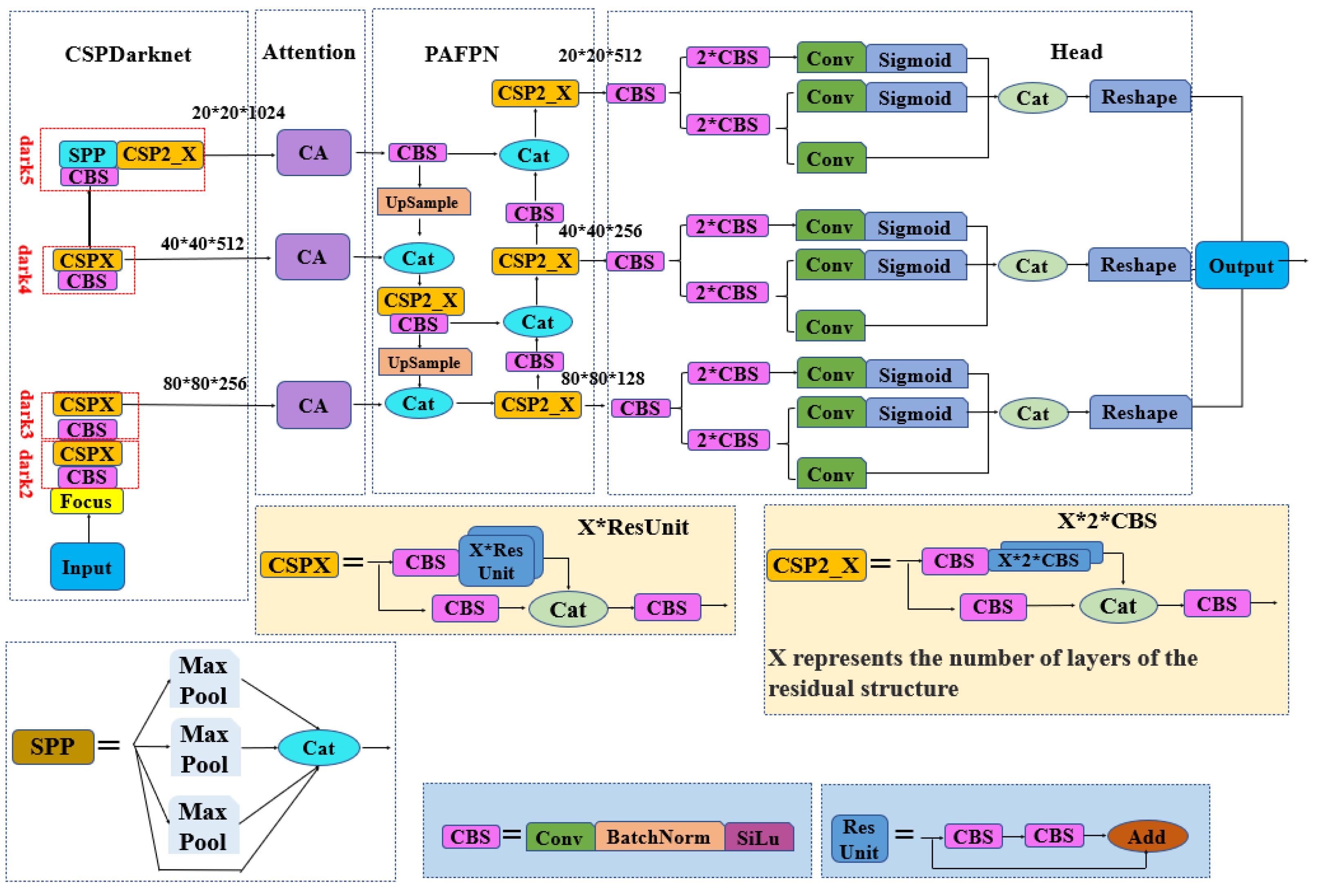
2.2.1. YOLOX Model

The YOLOX [44] model is a relatively new anchor-free object detection algorithm. Firstly, it uses two data augmentation methods at the input end, Mosaic and Mixup. Secondly, the backbone network is the same CSPDarknet structure as the v5 model, which consists of Focus, CBS, CSPX, and SPP. The Focus structure takes every other pixel value through slicing operations to expand the input channels, increasing the receptive field without increasing computational complexity. The model employs maximum pooling for multiscale feature fusion and also utilizes a top-down FPN (Feature Pyramid Network) and bottom-up PAN (Path Aggregation Network) to enhance feature extraction capabilities. Utilizing the FPN, the model obtains three effective feature layers tailored for detecting large-, medium-, and small-sized objects. These three feature layers are fed into the Head to obtain prediction information [45]. The Head uses a decoupled head, which first performs dimensionality reduction using a 1 × 1 convolution and then branches into two paths. One path handles the classification task, while the other path determines the presence of objects within the bounding boxes and their coordinate information [46].

2.2.2. Coordinate Attention Mechanism

The Coordinate Attention Mechanism [47] is an attention mechanism that takes into account both inter-channel relationships and positional information. It performs adaptive weighted average pooling along the channel and spatial dimensions, capturing the correlations between pixels at different positions to improve the accuracy of object detection. It consists of two specific steps: the embedding of positional information and generation of Coordinate Attention.

(1) Embedding of positional information. In order to facilitate the attention module to capture long-range dependencies with precise spatial positional information, global pooling can be decomposed into a pair of one-dimensional feature encodings. Specifically, for a given input X, we first use pooling kernels of sizes $(H,1)$ and $(1,W)$ along the horizontal and vertical coordinate directions to encode each channel. Therefore, the output of the cth channel with height h is represented as Equation (1):

$$z_c^h\left(h\right)={\displaystyle \frac{1}{W}}\sum _{0\le i\le W}{x}_c(h,i)$$

(1)

Similarly, the output of the cth channel with width w is represented as Equation (2):

$$z_c^w\left(w\right)={\displaystyle \frac{1}{H}}\sum _{0\le j\le H}{x}_c(j,w)$$

(2)

The two transformations mentioned above aggregate features along the two spatial directions, respectively, and return a pair of direction-aware attention maps.

(2) Coordinate Attention Generation. This module can better utilize the feature information generated by the aforementioned positional information embedding module, which possesses a global receptive field and precise positional information. It cascades the two feature maps generated by Equations (1) and (2) and then applies a shared 1 × 1 convolutional transformation function $F_1$, as shown in Equation (3):

$$f=\delta \left(F_1\left(\left[Z^{\hslash },Z^w\right]\right)\right)$$

(3)

In the equation, [•,•] represents the concatenation operation along the spatial dimension. $\delta$ is a non-linear activation function, and f is the intermediate feature map for spatial information in the horizontal and vertical directions. f is split into two independent tensors, $f^h$ and $f^w$, along the spatial dimension. Then, using two 1 × 1 convolutions, $F_h$ and $F_w$, feature maps $f^h$ and $f^w$ are transformed to have the same number of channels as input X, resulting in Equations (4) and (5):

$$g^h=\delta \left(F_h\left(f^h\right)\right)$$

(4)

$$g^w=\delta \left(F_w\left(f^w\right)\right)$$

(5)

Then, $g^w$ and $g^h$ are used as attention weights. Finally, the output of the Coordinate Attention Block Y is obtained as Equation (6):

$$y_c(i,j)=x_c(i,j)\times g_c^w\left(j\right)\times g_c^h\left(i\right)$$

(6)

2.2.3. The YOLOX Model Integrated with the Coordinate Attention (CA) Mechanism

To further enhance the feature extraction capability of the YOLOX-tiny model, optimizations were carried out by introducing the Coordinate Attention (CA) mechanism into the dark3, dark4, and dark5 parts of the feature extraction network CSPDarknet. This incorporation strengthens the model’s ability to extract pepper plant features, allowing the network to focus more on regions of interest. This means that the information weight of the target region is increased, while the weight of irrelevant information is reduced. The improved CA_YOLOX-tiny model’s network architecture is depicted in Figure 2.

2.2.4. Model Training Parameter Settings and Evaluation Metrics

During the experimental training, a cloud server with Ubuntu 20.04 as the operating system was used. The server was equipped with an Intel(R) Xeon(R) Platinum 8255C processor and an NVIDIA GeForce RTX 3080 GPU with 10 GB of VRAM. The processor had a clock speed of 2.5 GHz. The programming language used was Python 3.8, and the environment was set up with PyTorch 1.3 and CUDA 11.3. The improved CA_YOLOX-tiny model takes images with dimensions of $640\times 640$ pixels as input. The training was conducted for 200 epochs, with a batch size of 2. The Adam optimizer was chosen as the training optimization method, with an initial learning rate of 0.01 and a momentum factor of 0.937.

The evaluation metrics used to assess the performance of the detection model include Precision (P), Recall (R), Mean Average Precision (mAP), F1-Score (harmonic mean of Precision and Recall), Frames Per Second (FPS), model memory usage, and the size of the model’s best weights.

2.3. Obtaining Pepper Phenotypic Parameters

2.3.1. Phenotypic Parameter Extraction: Image Preprocessing

In order to obtain pepper phenotypic parameters quickly and accurately, it is necessary to preprocess the pepper images after performing multi-object detection. The specific steps are shown in Figure 3.

Step 1: Individual plant pruning based on Euclidean distance. In order to select the plant to be tested from the multiple detected plants, this study uses the Euclidean distance between the center point of the detection frame and the center point of the captured image as the judgment condition, and the detection frame where the center point with the smallest distance is selected is the plant to be tested, and then the location information of the plant to be tested can be known. The image can be cropped using the coordinate information of the target detection frame of the plant to be tested to obtain a single image of only the plant to be tested.

Step 2: Extraction based on HSV thresholding of pepper images. In order to facilitate obtaining binary images for subsequent measurements of plant height and stem thickness, this paper explores the method of extracting the green features of the target plants. Commonly used color models include the RGB model and the HSV model. After multiple experimental tests, it was found that the HSV model with Hmin = 35, Smin = 43, Vmin = 46, Hmax = 95, Smax = 255, and Vmax = 255 yields the best results. In comparing the effect of the RGB color model’s EXG super-green segmentation algorithm with the specified threshold segmentation method in the HSV color model, it was observed that the EXG super-green segmentation method under the RGB color model led to over-segmentation of pepper plants, causing damage to the target plants. On the other hand, the green threshold segmentation method under the HSV color model ensures the integrity of pepper plants to a great extent and exhibits better robustness. Therefore, this study selected the green threshold segmentation method under the HSV color model for pepper image plant extraction.

Step 3: Denoising and segmentation of individual plant images. The measurement of plant height and stem thickness relies mainly on the grayscale information of the images. Therefore, in this study, the color images obtained from the HSV threshold segmentation were converted into binary images, as shown in Figure 4a. Subsequently, the OTSU algorithm was applied to achieve foreground–background segmentation, highlighting the regions of interest. To eliminate noise interference and remove non-connected regions in the images, this study employed morphological opening and closing operations, as shown in Figure 4b, as well as connected region denoising methods, as shown in Figure 4c, to effectively process the images.

2.3.2. Plant Height and Stem Thickness Measurement Algorithm

Due to the disparity between the unit pixel size in images and the actual size in real life at different distances, the measurement and acquisition of pepper plant height and stem thickness rely on image-based methods. This necessitates the placement of a reference object during each measurement to establish the conversion relationship for unit pixel size, making the process cumbersome. To address this challenge, this study employed a parameter equation for converting the unit pixel size at different distances. The equation is derived by processing images of reference objects with known actual sizes and regular shapes, captured at various distances, using image segmentation techniques. It calculates the width of the reference object in terms of pixels within the image.Through the consideration of the shooting distance as the independent variable and the width of the reference object in pixels as the dependent variable, the equation was fitted to obtain the conversion factor for actual sizes. Through experimental validation, the correlation between the calculated values and the actual measurements reaches a highly accurate linear relationship with a correlation coefficient of 0.999. Consequently, the equation can effectively compute the conversion relationship for unit pixel sizes at different distances, eliminating the need for manual measurement and streamlining the process.

(1) The measurement method of plant height. In the preprocessed pepper binary image, the plants have connected regions. In this study, the actual height of the pepper plant could be obtained by calculating the number of pixels of the height of the minimum circumscribed rectangle of the connected area, combined with the pixel size conversion parameter equation, as shown in Equation (7):

$$H=\mathrm{perpixel}\text{\_}{\mathrm{size}}^{\ast }h$$

(7)

Here, perpixel_size is the actual size corresponding to the unit pixel at the specified distance, that is, the conversion ratio of the unit pixel. h is the number of pixels occupied by the pepper plant height in the image. H is the actual height of the pepper plant obtained after image processing.

(2) Measuring algorithm for stem thickness. To calculate the stem thickness, you first need to know the number of pixels that the main stem occupies in the image, and then multiply it with the unit pixel conversion ratio at a specified distance to obtain the width of the main stem of the pepper. The number of pixels that the main stem occupies in the image is shown in Equation (8):

$$w={\displaystyle \frac{{\sum }_{i=1}^m{w}_i}{n}}$$

(8)

In this context, i represents the number of rows occupied by the main stem in the digital image, $w_i$ denotes the number of pixels taken up by the main stem in each row of the digital image, and n stands for the total number of rows containing only thick stem pixels. The presence of leaves will cause $w_i$ in Equation (8) to include both the width of the leaves and the width of the main stem, as shown in Figure 5a. Therefore, in order to measure the thickness of the stem accurately, it is necessary to first address the interference caused by the presence of leaves.

For the convenience of research, this paper uses the local simulation diagram shown in Figure 5b to represent the local area selected by the red box in Figure 5a. Considering the pixels of each row in Figure 5b as a unit, we observe the following two situations: (1) there are both leaf pixels and thick stem pixels in the row; (2) there are only thick stem pixels and no leaf pixels in the row.

In observing the simulation diagram, it can be seen that the row containing only the thick stem pixels is composed of continuous 1s, and there is no 0 in the middle, while the row where the leaf pixels and the thick stem pixels exist at the same time is composed of multiple consecutive 1s, and there are 0s between the segments. Assume that the obtained binary image has a total of R rows and C columns, and for the above two situations, create a marker matrix $T_{(i,j)}$ to distinguish them, as shown in Equation (9):

$$T_{i,j}=\left\{\begin{array}{c}1,f\left(x_i,y_c\right)=0\mathrm{and}f\left(x_i,y_{c+1}\sim y_{c+k}\right)=1\hfill \\ \mathrm{and}f\left(x_i,y_{c+k}\sim y_j\right)=0\hfill \\ 0,\mathrm{others}\hfill \end{array}\right.$$

(9)

where i is the number of rows in the digital image, j is the number of columns in the digital image, c is a positive integer from 0 to j, with $c+k$ being less than j, and $T_{(i,j)}$ is the marker matrix. If case (1) occurs, there will be multiple pixel values of 1 in the row of marking matrix T; if case (2) occurs, only one pixel value of 1 will appear in the row of marking matrix T, and the remaining pixel values will be 0. Therefore, by summing the elements of each row of the marker matrix, we can know whether the row only contains pixels with thick stems, as shown in Equation (10):

$$T_i=\sum _{j=1}^n{T}_{i,j}$$

(10)

When $T_i$ = 1, the row only contains pixels with stem thickness, and all the pixels in the row can be considered to be stem-thick pixels; when $T_i$ != 1, the row contains both leaf pixels and stem-thick pixels, and the row needs to be discarded when calculating the stem thickness. Then, a statistical summation is performed on the stem-thick pixels. At the same time, it is necessary to count the number of rows occupied by the pixels of the stem thickness, and the number of pixels occupied by the average stem thickness is shown in Equation (8).

3. Experiment and Result Analysis

3.1. Model Comparison

In order to verify the superiority of the detection effect of the CA_YOLOX-tiny model proposed in this paper, the CA_YOLOX-tiny model was compared with the YOLOv4-tiny, YOLOv5-m, YOLOv7-tiny, and YOLOX-tiny models, and the IoU threshold was 0.5. The comparison experiment results are shown in

Table 1. Comparison of experimental results of each model.

Parameters	YOLOv4-tiny	YOLOv5-m	YOLOv7-tiny	YOLOX-tiny	Ours
mAP/%	86.40	93.19	88.50	93.49	95.16
Precision/%	97.84	99.74	99.42	97.90	98.46
Recall/%	79.20	85.79	73.63	89.17	89.20
F1-Score/%	88	92	85	93	94
Memory usage/M	5.874 M	21.056 M	6.014 M	5.033 M	5.055 M
Model’s size	22.40 M	80.64 M	23.10 M	19.40 M	19.50 M
FPS/(f·s−1)	16.4	4.3	13.3	11.7	10.7

* Bold values indicate the best performance.

.

It can be seen from Table 1 that CA_YOLOX-tiny achieves the best results in terms of mAP, Recall, and F1-score, reaching 95.16%, 89.2%, and 94%, respectively. Compared with the five models of YOLOv4-tiny, YOLOv5-m, YOLOv7-tiny, and YOLOX-tiny, the model proposed in this paper scored 8.76%, 1.97%, and 6.66% higher in mAP, respectively; 1.67%, 10%, 3.41%, 15.57%, and 0.03% higher in Recall; and 6%, 2%, 9%, and 1% higher in F1-score. Although the model in this paper does not achieve the best results in Precision, Params, optimal weight, and FPS, the model Precision in this paper is only 1.28% lower than the best result of YOLOv5-m; Params is only 0.022 M higher than the lowest result of YOLOX-tiny, which can be ignored; the best weight is only 0.1 M higher than the lowest of YOLOX-tiny; and FPS is tested with only the CPU, where CA_YO. The FPS of the LOX-tiny model is 10.7. In summary, the CA_YOLOX-tiny model based on CA attention proposed in this paper achieves obvious advantages in the pepper plant detection task.

In order to compare the performance of different pepper plant detection models more intuitively, the detection results of the CA_YOLOX-tiny model were compared with those of other detection models. The comparison results are shown in Figure 6.

Compared with the CA_YOLOX-tiny model proposed in this paper, other models have missed detection results. Among them, two strains were missed by YOLOv4-tiny, two strains were missed by YOLOv5-m, two strains were missed by YOLOv7-tiny, and one strain was missed by YOLOX-tiny. These missed plants belong to the situation of occlusion and serious adhesion. It can be seen that CA_YOLOX-tiny has a better detection effect on the above problems.

3.2. Plant Height Stem Diameter Measurement

In order to verify the feasibility of the method in this paper, this paper compares the plant height and stem diameter of pepper plants measured manually with the plant height and stem diameter obtained through image processing, and the accuracy of the method was tested using the error between the actual value and the algorithm measurement value. In this study, 20 peppers in different growth periods were selected for verification. Figure 7a,b, respectively, show the correlation between the measured values of plant height and stem diameter and the actual values.

Table 2. Measurement of plant height.

Number	Plant Height Measured by the Algorithm (cm)	Actual Plant Height (cm)	Error (cm)
1	21.62	21.00	0.62
2	20.70	21.10	0.40
3	21.77	22.30	0.53
4	26.82	26.50	0.32
5	18.07	18.50	0.43
6	20.32	21.10	0.78
7	20.53	20.20	0.33
8	22.22	22.50	0.28
9	22.88	22.50	0.38
10	19.94	20.30	0.36
11	20.84	21.50	0.66
12	22.11	21.50	0.61
13	22.09	22.60	0.51
14	19.38	20.00	0.62
15	24.48	24.60	0.12
16	20.65	21.30	0.65
17	21.05	21.30	0.25
18	22.96	22.60	0.36
19	30.98	31.00	0.02
20	21.16	21.80	0.64

and

Table 3. Measurement of stem thickness.

Number	Stem Thickness Measured by Algorithm (mm)	Actual Stem Thickness (mm)	Error (mm)
1	2.97	2.98	0.01
2	2.61	2.72	0.11
3	3.06	3.03	0.03
4	2.88	3.01	0.13
5	2.70	2.73	0.03
6	3.38	3.35	0.03
7	2.97	2.83	0.14
8	2.88	3.08	0.20
9	3.12	3.15	0.03
10	3.38	3.30	0.08
11	3.06	3.23	0.17
12	3.64	3.68	0.04
13	2.97	3.11	0.14
14	3.24	3.33	0.09
15	2.90	2.92	0.02
16	2.82	2.80	0.02
17	3.00	2.93	0.07
18	3.10	3.02	0.08
19	3.16	3.10	0.06
20	3.00	2.95	0.05

, respectively, show the error between the calculated values of plant height and stem diameter and the actual values.

The linear fitting results of the algorithm-measured plant height and the actual plant height are shown in Figure 7a. The obtained regression equation is $y=0.937x+1.579$ (the algorithm measured value is x; the actual plant height is y), the correlation coefficient ($R^2$) reaches 0.974, and the RMSE is controlled within 0.5 cm, indicating that there is a strong linear relationship between the two. It can be shown that the algorithm is feasible and effective for measuring pepper plant height and can replace manual measurement as an accurate estimate of the actual plant height. In addition, it can be seen from Table 2 that most of the errors generated by the plant height measurement algorithm are concentrated within 1 cm. After calculation, the average error is 0.443 cm, the maximum error is 0.78 cm, and the minimum error is 0.02 cm. Compared with the sample itself, these errors are within an acceptable range. This shows that the plant height measurement algorithm in this paper has high precision and can meet the measurement requirements of plant height under certain conditions.

The linear fitting results of the algorithm-measured stem thickness and the actual stem thickness are shown in Figure 7b. The obtained regression equation is $y=0.902x+0.32$ (the value of the algorithm measured stem thickness is x, and the actual stem thickness is y), the correlation coefficient ($R^2$) reached 0.842, and the RMSE was controlled within 0.1 mm, indicating that there is a strong linear relationship between the two. At the same time, it can illustrate the effectiveness of the algorithm, which can replace manual measurement as an accurate estimate of the actual stem thickness. In addition, it can be seen from Table 3 that most of the errors generated by the stem thickness measurement algorithm are concentrated within 0.2 mm, where the maximum error is 0.2 mm, the minimum error is 0.01 mm, and the average error is 0.077 mm.

4. Conclusions

Images of pepper plants were collected, and the Pepper-mini dataset was constructed by offline enhancement. At the same time, a unit pixel size conversion equation at different distances was fitted, which laid the foundation for the subsequent actual measurement of plant height and stem thickness. A measurement model of CA_YOLOX-tiny pepper plant height and stem diameter based on Euclidean distance was proposed. The model reached 95.16% in mAP, and can accurately locate a single target plant from multiple pepper plants in a complex environment, then complete the extraction of the plant to be tested through image processing operations such as threshold segmentation in the HSV color space and noise reduction in connected areas, and finally use the measurement algorithm of plant height and stem thickness to complete the precise measurement of the plant to be tested. Experiments show that the $R^2$ of the fitting equation between the measured value of plant height and stem diameter and the actual value reached 0.973 and 0.842, respectively, and the average errors were 0.443 cm and 0.0765 mm respectively, indicating that the proposed method can replace manual measurement to a certain extent. However, a limitation of this study is its primary focus on the phenotypic parameter measurement of pepper plants, with applicability to other crops yet to be validated. In practical agricultural production, different crops exhibit significant variations in growth morphology, color, texture, and other characteristics [48,49,50,51]. Therefore, models and methods that perform well on pepper plants may not be directly transferable to other crops. Future research should aim to extend the proposed approach to other crop species and verify its effectiveness and adaptability in measuring phenotypic parameters across diverse agricultural contexts. In addition, this study was mainly conducted in an indoor environment under controlled lighting and background conditions, which may not fully reflect the variability encountered in real-world agricultural scenarios. Future work will include field experiments under natural lighting to evaluate model robustness. Furthermore, we plan to explore multimodal data fusion [52] strategies by integrating RGB, depth, and thermal information, aiming to improve the accuracy and reliability of phenotypic trait estimation under complex field conditions.

References

1. Dobón-Suárez, A.; Zapata, P.J.; García-Pastor, M.E. A Comprehensive Review on Characterization of Pepper Seeds: Unveiling Potential Value and Sustainable Agrifood Applications. Foods 2025, 14, 1969. [Google Scholar] [CrossRef] [PubMed]
2. Pradeep, S.; Pabitha, C.; Kumar, T.R.; Joseph, J.; Mahendran, G.; Maranan, R. Enhancing pepper growth and yield through disease identification in plants using leaf-based deep learning techniques. In Hybrid and Advanced Technologies; CRC Press: Boca Raton, FL, USA, 2025; pp. 54–59. [Google Scholar]
3. Gerakari, M.; Katsileros, A.; Kleftogianni, K.; Tani, E.; Bebeli, P.J.; Papasotiropoulos, V. Breeding of Solanaceous Crops Using AI: Machine Learning and Deep Learning Approaches—A Critical Review. Agronomy 2025, 15, 757. [Google Scholar] [CrossRef]
4. Sanatombi, K. A comprehensive review on sustainable strategies for valorization of pepper waste and their potential application. Compr. Rev. Food Sci. Food Saf. 2025, 24, e70118. [Google Scholar] [CrossRef]
5. Chen, Y.; Wang, X.; Yang, W.; Peng, G.; Chen, J.; Yin, Y.; Yan, J. An efficient method for chili pepper variety classification and origin tracing based on an electronic nose and deep learning. Food Chem. 2025, 479, 143850. [Google Scholar] [CrossRef]
6. Ma, Y.; Zhang, S. YOLOv8-CBSE: An Enhanced Computer Vision Model for Detecting the Maturity of Chili Pepper in the Natural Environment. Agronomy 2025, 15, 537. [Google Scholar] [CrossRef]
7. Wang, R.F.; Su, W.H. The application of deep learning in the whole potato production Chain: A Comprehensive review. Agriculture 2024, 14, 1225. [Google Scholar] [CrossRef]
8. Jiang, L.; Rodriguez-Sanchez, J.; Snider, J.L.; Chee, P.W.; Fu, L.; Li, C. Mapping of cotton bolls and branches with high-granularity through point cloud segmentation. Plant Methods 2025, 21, 1–24. [Google Scholar] [CrossRef]
9. Yang, Z.Y.; Xia, W.K.; Chu, H.Q.; Su, W.H.; Wang, R.F.; Wang, H. A Comprehensive Review of Deep Learning Applications in Cotton Industry: From Field Monitoring to Smart Processing. Plants 2025, 14, 1481. [Google Scholar] [CrossRef]
10. Jiang, L.; Li, C.; Fu, L. Apple tree architectural trait phenotyping with organ-level instance segmentation from point cloud. Comput. Electron. Agric. 2025, 229, 109708. [Google Scholar] [CrossRef]
11. Fatchurrahman, D.; Hilaili, M.; Russo, L.; Jahari, M.B.; Fathi-Najafabadi, A. Utilizing RGB imaging and machine learning for freshness level determination of green bell pepper (Capsicum annuum L.) throughout its shelf-life. Postharvest Biol. Technol. 2025, 222, 113359. [Google Scholar] [CrossRef]
12. Zheng, X.; Shao, Z.; Chen, Y.; Zeng, H.; Chen, J. MSPB-YOLO: High-Precision Detection Algorithm of Multi-Site Pepper Blight Disease Based on Improved YOLOv8. Agronomy 2025, 15, 839. [Google Scholar] [CrossRef]
13. Qin, Y.M.; Tu, Y.H.; Li, T.; Ni, Y.; Wang, R.F.; Wang, H. Deep Learning for Sustainable Agriculture: A Systematic Review on Applications in Lettuce Cultivation. Sustainability 2025, 17, 3190. [Google Scholar] [CrossRef]
14. Tan, C.; Sun, J.; Song, H.; Li, C. A customized density map model and segment anything model for cotton boll number, size, and yield prediction in aerial images. Comput. Electron. Agric. 2025, 232, 110065. [Google Scholar] [CrossRef]
15. Meyer, G.E.; Davison, D.A. An electronic image plant growth measurement system. Trans. ASAE 1987, 30, 242–0248. [Google Scholar] [CrossRef]
16. Casady, W.; Singh, N.; Costello, T. Machine vision for measurement of rice canopy dimensions. Trans. ASAE 1996, 39, 1891–1898. [Google Scholar] [CrossRef]
17. Wang, Z.; Wang, R.; Wang, M.; Lai, T.; Zhang, M. Self-supervised transformer-based pre-training method with General Plant Infection dataset. In Proceedings of the Chinese Conference on Pattern Recognition and Computer Vision (PRCV), Urumqi, China, 18–20 October 2024; Springer: Singapore, 2024; pp. 189–202. [Google Scholar]
18. Chen, D.; Neumann, K.; Friedel, S.; Kilian, B.; Chen, M.; Altmann, T.; Klukas, C. Dissecting the phenotypic components of crop plant growth and drought responses based on high-throughput image analysis. Plant Cell 2014, 26, 4636–4655. [Google Scholar] [CrossRef]
19. Mora, M.; Avila, F.; Carrasco-Benavides, M.; Maldonado, G.; Olguín-Cáceres, J.; Fuentes, S. Automated computation of leaf area index from fruit trees using improved image processing algorithms applied to canopy cover digital photograpies. Comput. Electron. Agric. 2016, 123, 195–202. [Google Scholar] [CrossRef]
20. Zhu, T.; Ma, X.; Guan, H.; Wu, X.; Wang, F.; Yang, C.; Jiang, Q. A calculation method of phenotypic traits based on three-dimensional reconstruction of tomato canopy. Comput. Electron. Agric. 2023, 204, 107515. [Google Scholar] [CrossRef]
21. Polk, S.L.; Cui, K.; Chan, A.H.; Coomes, D.A.; Plemmons, R.J.; Murphy, J.M. Unsupervised diffusion and volume maximization-based clustering of hyperspectral images. Remote Sens. 2023, 15, 1053. [Google Scholar] [CrossRef]
22. Cui, K.; Li, R.; Polk, S.L.; Lin, Y.; Zhang, H.; Murphy, J.M.; Plemmons, R.J.; Chan, R.H. Superpixel-based and spatially-regularized diffusion learning for unsupervised hyperspectral image clustering. IEEE Trans. Geosci. Remote Sens. 2024, 62, 4405818. [Google Scholar] [CrossRef]
23. Chang-Tao, Z.; Rui-Feng, W.; Yu-Hao, T.; Xiao-Xu, P.; Wen-Hao, S. Automatic lettuce weed detection and classification based on optimized convolutional neural networks for robotic weed control. Agronomy 2024, 14, 2838. [Google Scholar] [CrossRef]
24. Cui, K.; Tang, W.; Zhu, R.; Wang, M.; Larsen, G.D.; Pauca, V.P.; Alqahtani, S.; Yang, F.; Segurado, D.; Fine, P.; et al. Real-time localization and bimodal point pattern analysis of palms using uav imagery. arXiv 2024, arXiv:2410.11124. [Google Scholar]
25. Wang, R.F.; Tu, Y.H.; Chen, Z.Q.; Zhao, C.T.; Su, W.H. A Lettpoint-Yolov11l Based Intelligent Robot for Precision Intra-Row Weeds Control in Lettuce. Available online: https://papers.ssrn.com/sol3/papers.cfm?abstract_id=5162748 (accessed on 30 April 2025).
26. Zhang, C.B.; Zhong, Y.; Han, K. Mr. DETR: Instructive Multi-Route Training for Detection Transformers. arXiv 2024, arXiv:2412.10028. [Google Scholar]
27. Bai, S.; Zhang, M.; Zhou, W.; Huang, S.; Luan, Z.; Wang, D.; Chen, B. Prompt-based distribution alignment for unsupervised domain adaptation. In Proceedings of the AAAI conference on artificial intelligence, Vancouver, BC, Canada, 26–27 February 2024; Volume 38, pp. 729–737. [Google Scholar]
28. Akdoğan, C.; Özer, T.; Oğuz, Y. PP-YOLO: Deep learning based detection model to detect apple and cherry trees in orchard based on Histogram and Wavelet preprocessing techniques. Comput. Electron. Agric. 2025, 232, 110052. [Google Scholar] [CrossRef]
29. Wu, A.Q.; Li, K.L.; Song, Z.Y.; Lou, X.; Hu, P.; Yang, W.; Wang, R.F. Deep Learning for Sustainable Aquaculture: Opportunities and Challenges. Sustainability 2025, 17, 5084. [Google Scholar] [CrossRef]
30. Cui, K.; Zhu, R.; Wang, M.; Tang, W.; Larsen, G.D.; Pauca, V.P.; Alqahtani, S.; Yang, F.; Segurado, D.; Lutz, D.; et al. Detection and Geographic Localization of Natural Objects in the Wild: A Case Study on Palms. arXiv 2025, arXiv:2502.13023. [Google Scholar]
31. Yang, B.; Gao, Z.; Gao, Y.; Zhu, Y. Rapid detection and counting of wheat ears in the field using YOLOv4 with attention module. Agronomy 2021, 11, 1202. [Google Scholar] [CrossRef]
32. Liu, J.; Wang, X. EggplantDet: An efficient lightweight model for eggplant disease detection. Alex. Eng. J. 2025, 115, 308–323. [Google Scholar] [CrossRef]
33. Rohith, D.; Saurabh, P.; Bisen, D. An integrated approach to apple leaf disease detection: Leveraging convolutional neural networks for accurate diagnosis. Multimed. Tools Appl. 2025, 1–36. [Google Scholar] [CrossRef]
34. Bi, C.; Bi, X.; Liu, J.; Xie, H.; Zhang, S.; Chen, H.; Wang, M.; Shi, L.; Song, S. Identification of maize kernel varieties based on interpretable ensemble algorithms. Front. Plant Sci. 2025, 16, 1511097. [Google Scholar] [CrossRef]
35. Ma, J.; Li, Y.; Liu, H.; Wu, Y.; Zhang, L. Towards improved accuracy of UAV-based wheat ears counting: A transfer learning method of the ground-based fully convolutional network. Expert Syst. Appl. 2022, 191, 116226. [Google Scholar] [CrossRef]
36. Baweja, H.S.; Parhar, T.; Mirbod, O.; Nuske, S. Stalknet: A deep learning pipeline for high-throughput measurement of plant stalk count and stalk width. In Proceedings of the Field and Service Robotics: Results of the 11th International Conference, Zurich, Switzerland, 12–15 September 2017; Springer: Cham, Switzerland, 2018; pp. 271–284. [Google Scholar]
37. Bendig, J.; Bolten, A.; Bennertz, S.; Broscheit, J.; Eichfuss, S.; Bareth, G. Estimating biomass of barley using crop surface models (CSMs) derived from UAV-based RGB imaging. Remote Sens. 2014, 6, 10395–10412. [Google Scholar] [CrossRef]
38. Li, Z.; Xu, R.; Li, C.; Tillman, B.; Brown, N. Robotic Plot-Scale Peanut Counting and Yield Estimation Using LoFTR-Based Image Stitching and Improved RT-DETR. In Proceedings of the 2024 ASABE Annual International Meeting, Anaheim, CA, USA, 28–31 July 2024; American Society of Agricultural and Biological Engineers: St. Joseph, MI, USA, 2024; p. 1. [Google Scholar]
39. Yuan, P.; Qian, S.; Zhai, Z.; FernánMartínez, J.; Xu, H. Study of chrysanthemum image phenotype on-line classification based on transfer learning and bilinear convolutional neural network. Comput. Electron. Agric. 2022, 194, 106679. [Google Scholar] [CrossRef]
40. Vit, A.; Shani, G.; Bar-Hillel, A. Length phenotyping with interest point detection. In Proceedings of the IEEE/CVF Conference on Computer Vision and Pattern Recognition Workshops, Long Beach, CA, USA, 15–20 June 2019. [Google Scholar]
41. Chen, M.; Liao, J.; Zhu, D.; Zhou, H.; Zou, Y.; Zhang, S.; Liu, L. MCC-Net: A class attention-enhanced multi-scale model for internal structure segmentation of rice seedling stem. Comput. Electron. Agric. 2023, 207, 107717. [Google Scholar] [CrossRef]
42. Li, Z.; Xu, R.; Li, C.; Munoz, P.; Takeda, F.; Leme, B. In-field blueberry fruit phenotyping with a MARS-PhenoBot and customized BerryNet. Comput. Electron. Agric. 2025, 232, 110057. [Google Scholar] [CrossRef]
43. Wang, B. Zero-exemplar deep continual learning for crop disease recognition: A study of total variation attention regularization in vision transformers. Front. Plant Sci. 2024, 14, 1283055. [Google Scholar] [CrossRef]
44. Ge, Z.; Liu, S.; Wang, F.; Li, Z.; Sun, J. Yolox: Exceeding yolo series in 2021. arXiv 2021, arXiv:2107.08430. [Google Scholar]
45. Li, Y.; Li, J.; Luo, L.; Wang, L.; Zhi, Q. Tomato ripeness and stem recognition based on improved YOLOX. Sci. Rep. 2025, 15, 1924. [Google Scholar] [CrossRef]
46. Miao, W.; Shen, J.; Xu, Q.; Hamalainen, T.; Xu, Y.; Cong, F. SpikingYOLOX: Improved YOLOX Object Detection with Fast Fourier Convolution and Spiking Neural Networks. In Proceedings of the AAAI Conference on Artificial Intelligence, Philadelphia, PA, USA, 25 February–4 March 2025; Volume 39, pp. 1465–1473. [Google Scholar]
47. Hou, Q.; Zhou, D.; Feng, J. Coordinate attention for efficient mobile network design. In Proceedings of the IEEE/CVF Conference on Computer Vision and Pattern Recognition, Nashville, TN, USA, 20–25 June 2021; pp. 13713–13722. [Google Scholar]
48. Tan, C.; Sun, J.; Paterson, A.H.; Song, H.; Li, C. Three-view cotton flower counting through multi-object tracking and RGB-D imagery. Biosyst. Eng. 2024, 246, 233–247. [Google Scholar] [CrossRef]
49. Tan, C.; Li, C.; Sun, J.; Song, H. Three-View Cotton Flower Counting through Multi-Object Tracking and Multi-Modal Imaging. In Proceedings of the 2023 ASABE Annual International Meeting, Omaha, NE, USA, 9–12 July 2023; American Society of Agricultural and Biological Engineers: St. Joseph, MI, USA, 2023; p. 1. [Google Scholar]
50. Xu, R.; Li, C. A review of high-throughput field phenotyping systems: Focusing on ground robots. Plant Phenomics 2022, 2022, 9760269. [Google Scholar] [CrossRef]
51. Jiang, Y.; Li, C. Convolutional neural networks for image-based high-throughput plant phenotyping: A review. Plant Phenomics 2020, 2020, 4152816. [Google Scholar] [CrossRef] [PubMed]
52. Yang, Z.X.; Li, Y.; Wang, R.F.; Hu, P.; Su, W.H. Deep Learning in Multimodal Fusion for Sustainable Plant Care: A Comprehensive Review. Sustainability 2025, 17, 5255. [Google Scholar] [CrossRef]
Figure 1. Partial pepper plant data.
Agriengineering 07 00209 g001
Figure 2. Improved CA_YOLOX-tiny model.
Agriengineering 07 00209 g002
Figure 3. Image preprocessing for phenotypic parameter extraction.
Agriengineering 07 00209 g003
Figure 4. Comparison of effect pictures before and after treatment.
Agriengineering 07 00209 g004
Figure 5. Binary map of pepper phenotype.
Agriengineering 07 00209 g005
Figure 6. Detection effect comparison chart.
Agriengineering 07 00209 g006
Figure 7. (a) Scatter diagram of plant height measurement. (b) Scatter diagram of stem thickness measurement.
Agriengineering 07 00209 g007