Article

Hierarchical Stratification for Spatial Sampling and Digital Mapping of Soil Attributes

School of Agricultural Engineering, Universidade Estadual de Campinas—UNICAMP, Campinas 13083-875, SP, Brazil
*
Author to whom correspondence should be addressed.
AgriEngineering 2025, 7(1), 10; https://doi.org/10.3390/agriengineering7010010
Submission received: 1 November 2024 / Revised: 2 December 2024 / Accepted: 24 December 2024 / Published: 2 January 2025

Abstract

:
This study assessed whether stratifying agricultural areas into macro- and micro-variability regions allows targeted sampling to better capture soil attribute variability, thus improving digital soil maps compared to regular grid sampling. Allocating more samples where soil variability is expected offers a promising alternative. We evaluated two sampling densities in two agricultural fields in Southeast Brazil: a sparse density (one sample per 2.5 hectares), typical in Precision Agriculture, and a denser grid (one sample per hectare), which usually provides reasonable mapping accuracy. For each density, we applied three designs: a regular grid and grids with 25% and 50% guided points. Apparent soil magnetic susceptibility (MSa) delimited macro-homogeneity zones, while Sentinel-2’s Enhanced Vegetation Index (EVI) identified micro-homogeneity, guiding sampling to pixels with higher Fuzzy membership. The attributes assessed included phosphorus (P), potassium (K), and clay content. Results showed that the 50% guided sample configuration improved ordinary kriging interpolation accuracy, particularly with sparse grids. In the six sparse grid scenarios, in four of them, the grid with 50% of the points in regular design and the other 50% directed by the proposed method presented better performance than the full regular grid; the higher improvement was obtained for clay content (RMSE of 54.93 g kg−1 to 45.63 g kg−1, a 16.93% improvement). However, prior knowledge of soil attributes and covariates is needed for this approach. We therefore recommend two-stage sampling to understand soil properties’ relationships with covariates before applying the proposed method.

1. Introduction

Sampling planning is a critical step in investigating the spatial variability of soil properties, and soil mapping accuracy is linked to sampling reliability. Agricultural areas are non-uniform, and soil variability can be found even in small areas [1]. Therefore, decision-making and input application must assume the existence of spatial variability. That is, application should be conducted at variable rates according to the demand and availability of nutrients in each situation, aiming to increase crop yield potential without depleting natural resources.
Soil fertility mapping for phosphate and potassium fertilizer prescriptions at variable rates has been performed using regular grid sampling [2]. Such regular grids emphasize uniform spatial coverage, ensuring a good representation of the entire field at regularly spaced intervals. This coverage provides an equal sampling grid in the area, especially favoring mapping when there is no prior knowledge of the area [3]. However, such equal distance in sparse grids can impair variogram modeling, compromising the characterization of the nugget effect, as there are no points at short distances [4]. In sampling planning, the sample amount usually varies according to the financial and operating constraints established by the practitioners. In Brazil, the sampling grid size varies widely depending on the region and the producer profile, and sampling grids with densities sparser than one sampling point every two hectares have been widely used [5]. However, this typical management contradicts recommendations for ideal grid size, which should be based on the variability of attributes of interest rather than financial constraints [6,7]. It may compromise the response of the fertilizer application rates, making it necessary to find solutions that circumvent this problem.
Studies have been focusing on optimizing sampling grids to obtain more accurate digital soil maps [8], especially in situations of low sampling density [9]. Some approaches are based on targeting sampling points using auxiliary terrain information, which exhibits spatial relationships with the soil variables to be mapped. Subdividing fields into smaller areas and guiding sampling locations with the assistance of auxiliary variables has proven to be a promising alternative to improve soil mapping accuracy [10,11]. Wang et al. [12] used stratification techniques based on covariates derived from Digital Elevation Model (DEM) data to infer soil macro-variability, called macro-zones, allowing the identification of higher-heterogeneity areas. Subsequently, they subdivided these macro-zones into micro-zones and guided sampling points to them, achieving higher mapping accuracy than when it is exclusively based on regular grids. Therefore, dividing the area to be mapped into sampling zones to infer soil macro- and micro-variability becomes a promising approach, as these areas represent sub-regions of a field with some homogeneity among attributes. However, relying solely on topography data can be limited in areas with gentle relief and high anthropic influence (soil management). In this context, apparent soil magnetic susceptibility (MSa) and vegetation indices (VI), obtained through remote sensing, can be alternatives to MDE products. These variables have a direct relationship with soil attributes, are easy to obtain, offer high resolution [13,14,15], and provide economic advantages. The cost associated with sampling based on MSa and VI is comparable to mapping using a regular grid, as satellite images are generally obtained for free, and MSa readings do not require repeated measurements, given that it is a temporally stable variable. Another issue is that this method of sampling point allocation results in an irregular grid, which may impair spatial interpolation [3,10].
Therefore, studying different sampling grid sizes and the percentage of points to be targeted is necessary to determine the sampling designs that produce better mapping results. Our hypothesis is that stratifying fields into hierarchical levels of homogeneity zones based on environmental covariates allows for the representation of local soil variability and, thus, can be useful information to guide soil sampling points. In this context, this research aimed to test whether guiding sampling points based on macro- and micro-zones allow for more accurate soil property maps than maps originating from the traditional regular grid. In addition, this study aimed to evaluate whether sample density affects the results of such a target-sampling approach.

2. Materials and Methods
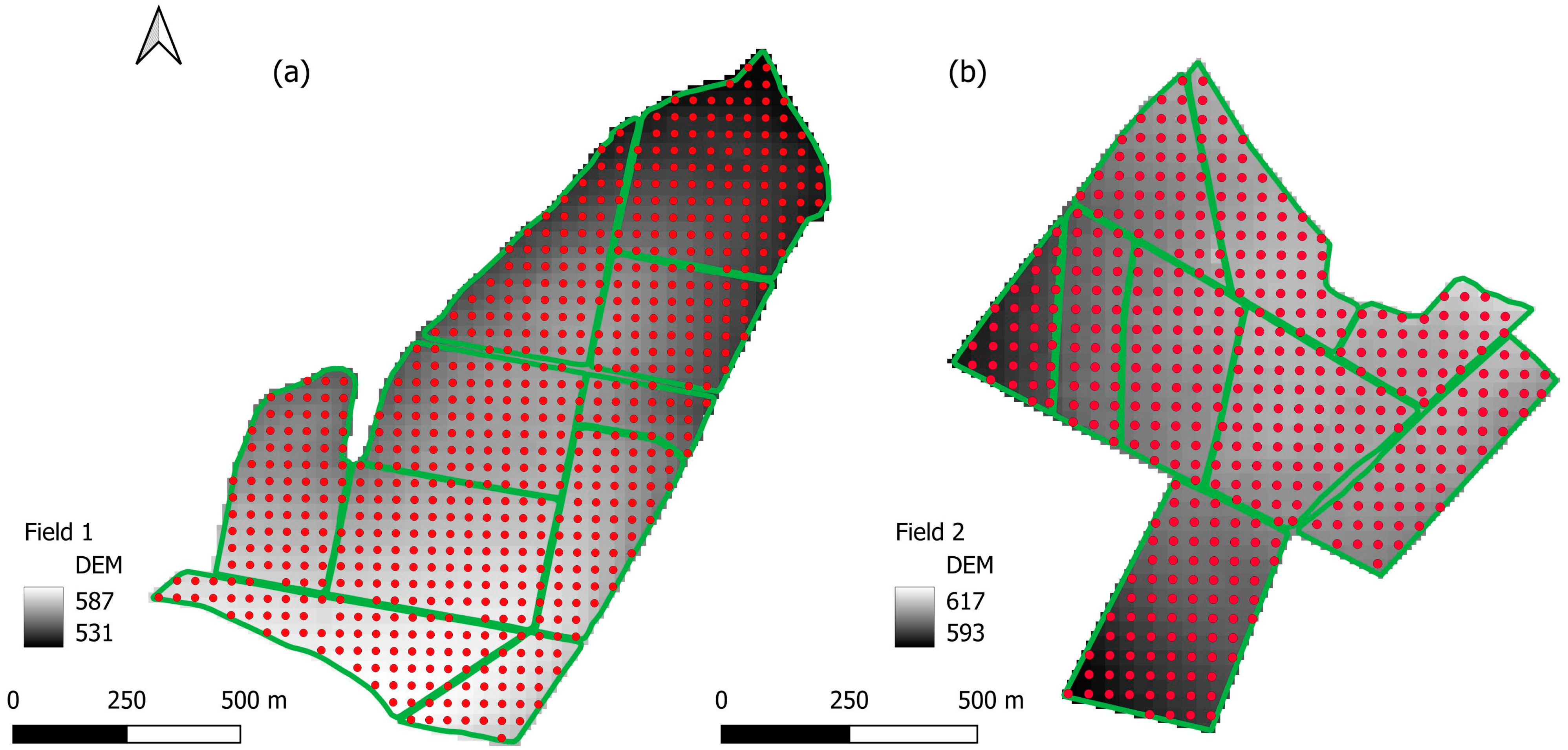
This study was conducted in two agricultural areas located in the state of São Paulo, Brazil. We used two covariates (soil and plant) to determine the variability of the area, subdividing it into macro- and micro-zones. Based on the area variability, previously dense soil sampling allowed different simulations on how to allocate sampling points in two densities (one sample per hectare and one sample every 2.5 hectares), integrating regular grid with targeted points in different percentages (25 or 50%), according to the delineated zones. We created maps of the soil attributes using ordinary kriging from the samples selected in each grid simulation. The quality of the maps was compared by the correlation, RMSE, and RPIQ of the actual values of soil attributes at the external validation points randomly distributed in the study areas.

2.1. Study Areas

The first study area, called Field 1 (Figure 1a), has 107 hectares and is in the municipality of Cosmópolis, state of São Paulo, Brazil, at coordinates 22°41′55.16″ S and 47°10′34.15″ W. The climate is classified in the Köppen system as Cfa, a subtropical climate with hot summers, a mean annual precipitation of 1400 mm, and a mean annual temperature of 20–22 °C. The terrain is gently wavy, and the predominant soil is an Oxisol (Latossolo Vermelho distrófico according to the Brazilian Soil Classification System [16]), with a texture ranging from clayey to very clayey. Grain cultivation is predominant in the area, with soybean planting in the first growing season and intercropping between oat and grain sorghum in the second.
The second study area, Field 2 (Figure 1b), has 72 hectares and is in the municipality of Sales Oliveira, state of São Paulo, Brazil, at coordinates 20°51′42″ S and 47°57′15″ W. The soil type in the region is the same in Field 1, with a very clayey texture, and the climate is classified in the Köppen system as Cwa, a humid subtropical climate with a sizzling summer, a mean annual temperature of 22 °C, and a mean annual precipitation of approximately 1300 mm. The field has a history of sugarcane cultivation and has been worked for ten years without reform (no new planting).

2.2. Soil Sampling

A dense soil sampling was collected in both study areas, with a 40 × 40-m regular sampling grid corresponding to six soil samples per hectare (reference grid—Figure 1). Each sampling point is a composite sample from six subsamples collected within a radius of five meters from the central point using an automated drill installed on a quad bike. This robust sampling density of the reference grid allowed the simulation of different sampling designs within the areas. The samples in Field 1 were collected at a depth of 0 to 20 cm, as this is the recommended depth for diagnosing soil fertility in grain-producing areas, while the sampling depth in Field 2 was 0 to 25 cm, as the recommended sampling depth for sugarcane crop [17]. The composite samples were sent to the same commercial soil analysis laboratory to determine chemical and physical analyses. For this study, we used three soil attributes due to their relevance to crop development and the extensive usage by precision agriculture practitioners for variable-rate fertilizer application: available phosphorus (P—mg dm−3) [18], potassium (K—mmolc dm−3) [19], and clay content (g kg−1) [20]. Table 1 shows the descriptive statistics of the soil analysis.

2.3. Field Covariates

The proposed methodology aimed to infer the variability of the study areas using the macro- and micro-zones. The purpose of dividing the macro-regions was to infer homogeneous zones in terms of soil and subdivide these zones into micro-regions that represent the crop’s response to soil variability to target the sampling points. The covariate used to delimit the homogeneous macro-zones throughout the study areas was the apparent soil magnetic susceptibility (MSa). A historical series of satellite images was used to obtain the micro-regions and infer the homogeneity of the vegetation across the growing seasons (Figure 2).
MSa is a physical property of matter that depends on the magnetic moments of atoms [21]. In soil, MSa is influenced by the amount of magnetic minerals and is mainly controlled by the concentrations of magnetite and maghemite [22]. The MSa application in soil has been the subject of studies in agriculture, as it allows the identification and characterization of homogeneous areas [23], which can be used in the creation of management zones due to the correlation with agronomic properties [24], synthesizing information on the spatial variability of the soil. We used MSa data obtained at a depth of up to 37.5 cm from the EM38-MK2 sensor (Geonics Limited, Mississauga, ON, Canada), which was towed by a quad bike with passes every 30 m. This sensor has the operating capacity to obtain a large amount of data (approximately 150 points per hectare) and cover large areas [13]. We created continuous raster files using ordinary kriging to obtain a spatialized MSa distribution in both areas.
Orbital remote sensing was the adopted alternative to characterize crop variability across the study areas and identify regions of micro-variability. Using vegetation indices through remote sensing provides information on plant health and vigor, which may be related to soil fertility [25,26]. In this sense, we used EVI (Enhanced Vegetation Index) (Equation (1)), which is an index that aims to reduce the saturation problem presented by NDVI while minimizing the effects of soil and atmosphere, presenting a high response to plant phonological changes [26]. EVI has proven effective when plant vigor is high and has been used to infer crop yield [14,15,27,28]. Sentinel-2 images from the last five years of the areas (2019–2023), with one image at the annual vegetative peak for each growing season (Table 2), were used for this study. Field 1 had no good-quality image to represent the vegetative peak of 2019 (presence of clouds); for this reason, we used two images in 2022, with the second image corresponding to the peak of the second growing season of the year. The mean EVI value was calculated for each pixel from the five images, resulting in a synthetic image for each area.
EVI = 2.5 × (NIR − RED)/(NIR + 6 × RED − 7.5 × BLUE + 1)
where NIR is the reflectance in the near-infrared band (Sentinel-2 Band 08), RED is the reflectance in the red band (Sentinel-2 Band 04), and BLUE is the reflectance in the blue band (Sentinel-2 Band 02).

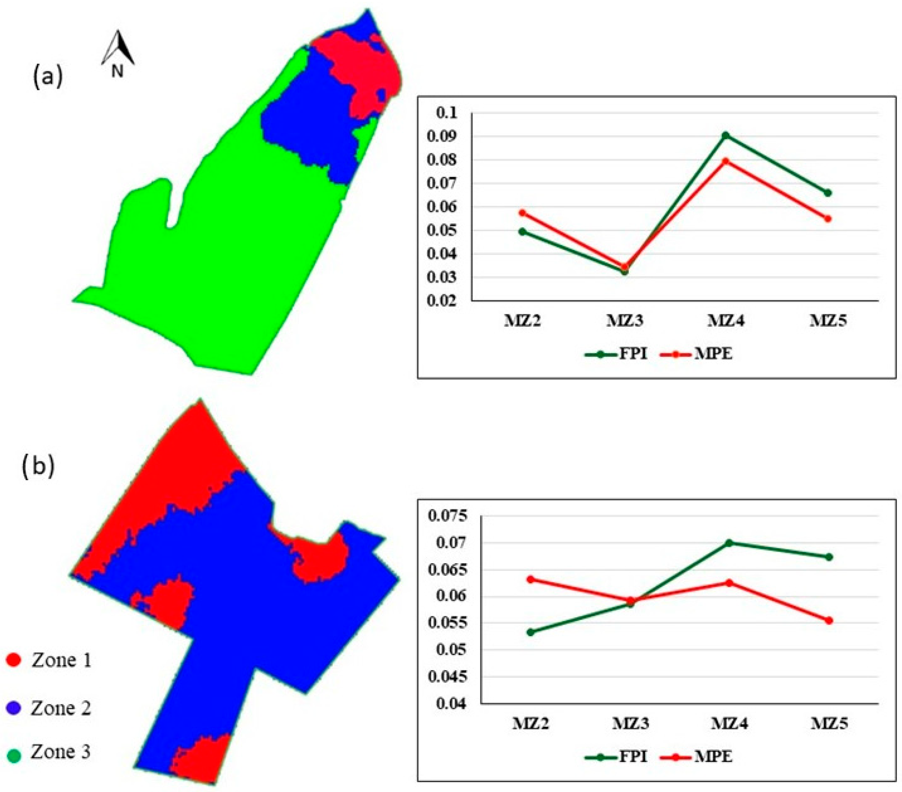
2.4. Inference of Soil Macro-Homogeneity

The areas were divided based on the MSa raster through c-means cluster analysis to create homogeneous macro-zones [29,30]. The selection of the ideal number of zones was based on the simultaneous analysis of the Fuzzy Performance Index (FPI) [31] and the Modified Partition Entropy (MPE) [32]. FPI reflects the degree of segregation between the observations and the formed clusters, while MPE expresses the degree of disorder established between the clusters, providing a comprehensive view of the resulting structure. The adequate number of clusters was determined based on the transition point in the curve, which indicated a stabilization in the spatial heterogeneity of the data so that the curve became smooth and the marginal gain with the increased number of zones became unnecessary. The minimal point at which a sharp change in the slope of the curve occurred was identified as the ideal number of clusters. Thus, we obtained the total number of three clusters for Field 1 and two for Field 2 (Figure 3), with each of them consisting of a zone based on MSa.

2.5. Determination of the Ideal Number of Points per Homogeneous Macro-Zone

The ideal number of points to be targeted per zone was determined based on the MSa variability (coefficient of variation—CV%) and the size of each zone. Thus, the larger the area and the higher the CV, the more points the zone received. The formula that determined the number of points was adapted from Wang et al. [12] (Equation (2)), which starts from an arbitrarily defined number of samples, which is usually based on the investment released for the survey. In this sense, two sampling densities were explored: (1) one point per hectare, which is often considered a target density, and (2) one sample every two and a half hectares, which is often adopted in field practice to make the survey viable due to the costs involved in sampling and laboratory analysis. Both sampling densities were targeted at 25% and 50% of the total points sampled in the grid (Table 3). The number of points was rounded to the nearest integer.
SNh = SN × Ah × CVh/∑Ah × CVh
where SNh is the number of points in each macro-zone, SN is the number of samples to be targeted in the total area, arbitrarily defined, Ah is the area of the macro-zone under study, and CVh is the coefficient of variation of MSa in each macro-zone.

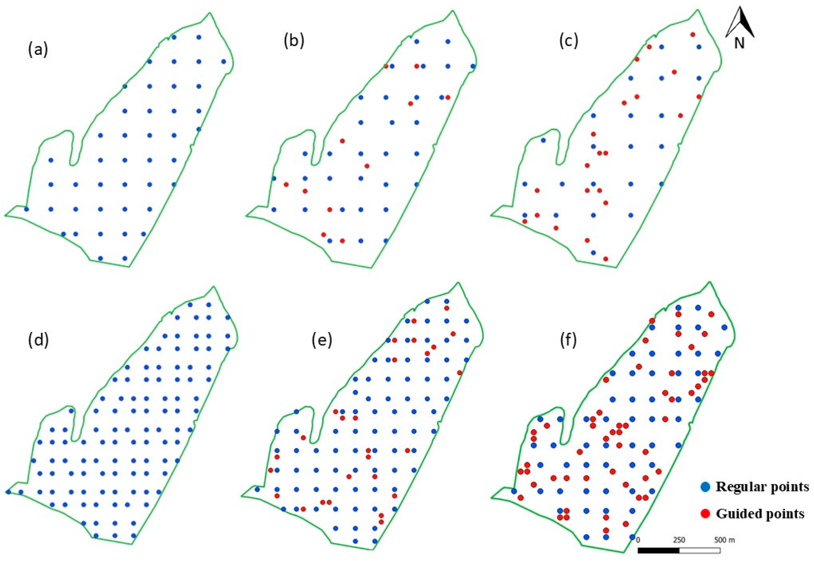
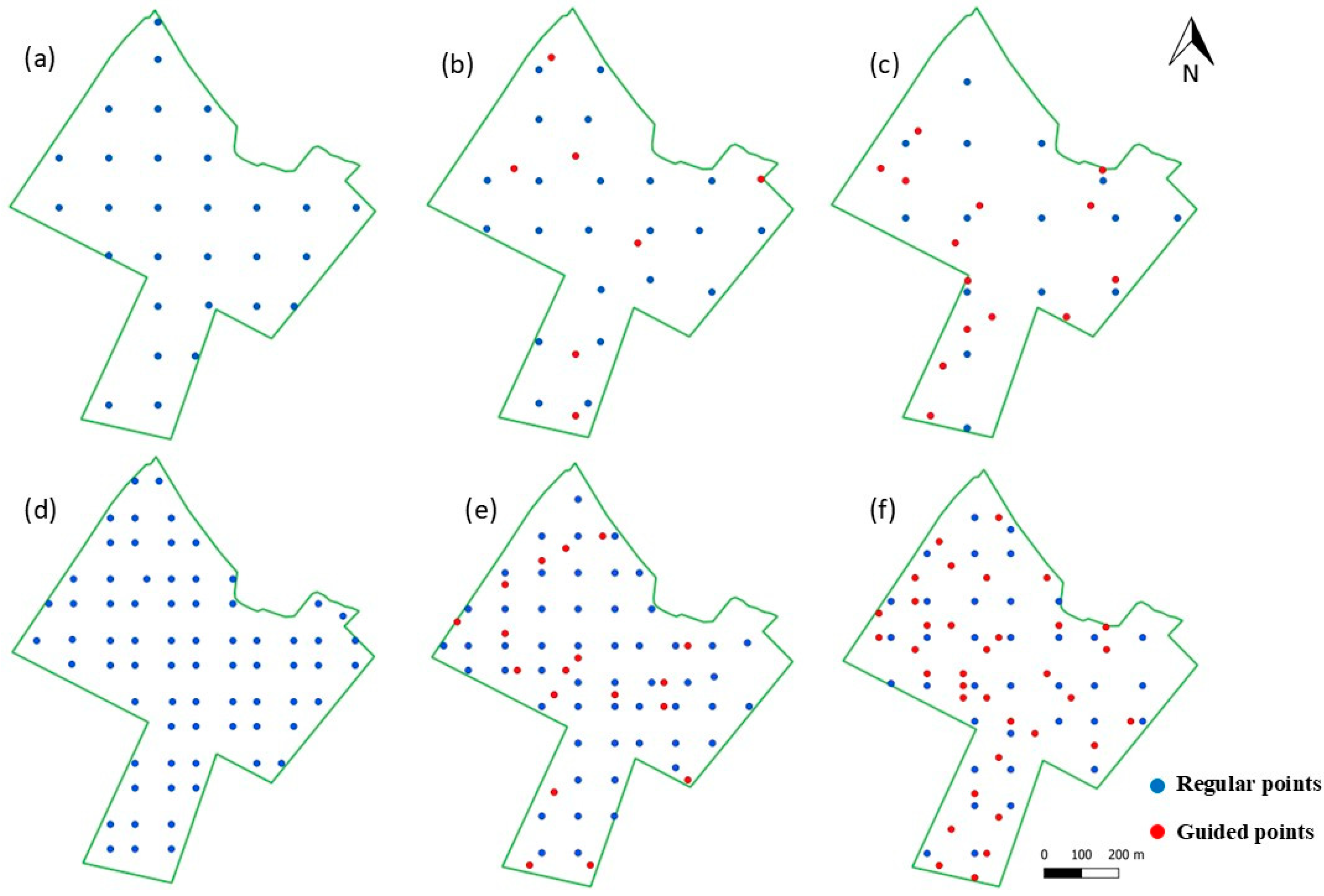
2.6. Inference of Soil Micro-Homogeneity and Location of Targeted Sampling Points

The macro-zones were divided into micro-zones to subdivide the homogeneous zones into smaller regions and indicate the collection sites for each soil sample. For such, we performed the Fuzzy c-means (FCM) clustering method [33] on the synthetic EVI images to create the homogeneous micro-zones. This approach allowed the subdivision of the macro-homogeneity zones originating from the MSa into homogeneous micro-zones of plant vigor. The number of micro-zones was defined by the number of samples indicated by Equation (2) and shown in Table 3. Thus, each micro-zone received one sample point. Therefore, the pixels of the zones generated by the Fuzzy c-means clustering have a dynamic classification and can have different degrees of relevance in each cluster (micro-zone) for each pixel on the map [34]. Thus, seeking to sample the location with the highest probability of representing the micro-zone in question, the pixel with the relevance value closest to one, i.e., 100% certainty, in each micro-zone was adopted as the sample point selected from the reference grid.

2.7. Interpolation

Both sampling densities were configured in three sampling designs after allocating the guided sampling points: a completely regular grid and two other grids combining regular and guided points, comprising 25% and 50% of guided points (Figure 4 and Figure 5), which, subsequently, underwent the process of generating maps by spatial interpolation. For this, ordinary kriging was used following all the precepts of variogram modeling suggested by Oliver and Webster [35].

2.8. Analysis of Results

The external validation procedure was adopted to evaluate whether targeting samples based on the proposed methodology improves the soil fertility maps’ accuracy compared to the regular sampling grid with the same number of total samples. To this end, the sampling points from the reference grid not used in the sampling scenarios worked as validation samples, totaling 273 samples for Field 1 and 212 for Field 2. The interpolation values of the different soil properties were extracted for the coordinates of these external validation points, and thus, the actual values were compared with those predicted from the following metrics: root mean square error (RMSE), Spearman’s correlation coefficient (r), and the ratio of performance to interquartile distance (RPIQ) [36]. RPIQ were interpreted following the classes suggested by Nawar and Mouazen [37]: excellent model (RPIQ > 2.5), very good model (2.5 > RPIQ > 2.0), good model (2.0 > RPIQ > 1.7), regular model (1.7 > RPIQ > 1.4), and poor model (RPIQ < 1.4).
In addition, the adjustment of variograms was explored to identify whether the increase in the percentage of guided samples improved the ability to capture soil spatial variability. Furthermore, the Moran index [38] was also calculated for each field to infer whether the soil properties’ spatial cluster influenced the sampling optimization results.

3. Results and Discussion

The sampling designs influenced the mapping performance of soil attributes in the two studied areas (Table 4). For Field 1, the one sample per hectare grid with 50% of guided samples demonstrated higher accuracy than the regular. However, regardless of the sampling design, available P prediction was inefficient due to its low spatial dependence and randomness (Table 5). For Field 2, the one sample per hectare grid with regular sampling points was more efficient in mapping all analyzed soil attributes. On the other hand, guiding sample points based on the hierarchical zones in the sparse grid (one sample every 2.5 hectares) was crucial to improving predictions on both fields. It shows that such a guided sampling approach is more likely to generate returns when the sampling grid is sparser (lower density). These results highlight the need to adapt sampling strategies to maximize mapping accuracy and optimize the resources available for efficient management.

3.1. Clay Content Mapping

3.1.1. One Sample per Hectare

The one sample per hectare grid with 50% of guided points provided the best clay content prediction in Field 1 (Table 6). The RMSE was 31.12 g/kg for the grid with 50% of guided points, 38.01 g/kg for the regular grid, and 39.23 g/kg for the grid with 25% of guided points. This difference of 8.17 g/kg between the highest and lowest RMSE values is considered low, given that the variation of the total sampling data ranges from 108 to 750 g/kg of clay (Table 1). On the other hand, the best results for Field 2 were found with the regular grid (Table 6), with the RMSE for clay content showing slightly better results, with a value of 31.07 g/kg, while the error for the grid with 50% of guided points was 31.12 g/kg, followed by 33.88 g/kg for the grid with 25% of guided points. However, these values are remarkably close, indicating a slight difference between the sampling approaches. This similarity may be associated with the homogeneity of the soil in Field 2, as evidenced by the low range of the values observed in the reference dataset (Table 1). Moreover, this difference between the fields is evident when analyzing the predicted versus observed values in Table 5, with a correlation of 0.54 for the best scenario in Field 2 and correlations of up to 0.93 for Field 1 (Table 6). However, despite the differences in the prediction performance in both fields, the grids with 50% of guided points delivered the best results for mapping this attribute (higher RPIQ) (Table 4). Thus, guided sampling is a viable alternative for mapping, especially when there are smaller and more prominent spots that the distance between points on the regular grid cannot capture. However, when the variability of the mapped attribute is low, in general, both forms of point allocation characterize the target attribute similarly.

3.1.2. One Sample per 2.5 Hectares

Targeting sample points was more effective for mapping in both fields when considering the characterization of clay through the grid of one sample point for every 2.5 hectares (Table 5). The reduction in sampling uncertainty was pronounced when targeting the points. In Field 1, where there is considerable variation in clay contents (Table 1) and spatial dependence is high, as evidenced by the Moran index (Table 5), guiding 50% of points resulted in more accurate predictions. The RPIQ index suggests that only the model with 50% of guided points is considered excellent (Table 4) for this sampling density in this field. Thus, a 2.5 ha grid could be enough to accurately map the clay content in Field 1, as it is in the same model adjustment class as the grids of one sample per hectare.
Moreover, for Field 1, the results show that the targeting in this sample configuration became more efficient in this field due to the correlation between clay and auxiliary variables. MSa presented a significant inverse correlation with clay (r = −0.62), while the synthetic EVI image also showed a considerable inverse correlation (r = −0.49) (Table 7). Thus, the 50% guided grid is a better option for soil maps when there is a correlation between the covariates and the primary attribute.
For Field 2, guiding 25% of sample points was more effective for clay content mapping (Table 6). Unlike Field 1, the correlation between the covariates and clay content suggests that the improvement was unrelated to the guiding method, as there was no clear correlation between the covariates and the attribute (Table 7). In the 2.5 ha grid, the distance between the sample points was approximately 158 m, while variogram parameters for the reference grid showed a range of 220 m (Table 5), indicating a short-range variability of this attribute. This pattern is corroborated by the Moran index, which also suggests a smaller spatial clustering when compared to Field 1 (Table 5). Previous studies have pointed out that the distribution of random points within a regular grid tends to reduce mapping errors compared to a completely regular grid [8]. The results of this study are aligned with our findings because the targeting was effective even in the absence of a clear relationship between the target attribute and the covariate, as it prioritized spatial coverage at 75% of regular points, while 25% targeted allowed points at shorter distances, thus improving the interpolation accuracy. In contrast, a higher loss of equidistance between points is observed when targeting 50% of points, generating the worst results between the three grid designs for Field 2. Clay interpolation performance was considered “good” (RPIQ = 1.78) even for the reference grid of six points per hectare but “regular” and “bad” for the other grid designs, regardless of the density (Table 4). The low variability of clay content in Field 2 makes the targeting of 50% of sample points inefficient, as the methodology demands attribute variability and correlation between it and the covariate, which was not found in this study. Thus, targeting is not indicated to map clay in a sparse grid under low variability conditions and without correlation with the covariate. In this situation, the regular sample grid is recommended.

3.2. Phosphorus Mapping

3.2.1. One Sample per Hectare

The chemical attributes showed a discrepancy between the results for the two experimental fields. The phosphorus content available along Field 1 presented reduced spatial variability, i.e., much of the data variability is not a function of its location, which can be verified by the result of the leave-one-out cross-validation of the ordinary kriging (Table 5) even for the reference dataset (650 samples, six samples per hectare). The Moran index also had low data grouping (Table 5), and the model performance by the RPIQ index was considered poor for all scenarios (Table 4). In addition, the correlation between the actual and predicted values for all grids ranged from 0.09 to 0.3, demonstrating the inefficiency of interpolation in mapping the attribute spatial behavior. These results show that the high sample density does not always generate good fertility maps. This low spatial dependence and high randomness between soil samples is often observed for available P and has already been reported in several studies [39,40,41]. Random and non-clustered behavior becomes even more noticeable in grain-producing areas, as P fertilization is usually required in high quantities, and the P that is not exported by the crop tends to remain in the labile P pool due to its low mobility in the soil profile [17], as Brazilian soils are poor in P and have a strong interaction with clay minerals. Although these factors result in the application of fertilization in high quantities, phosphorus is the macronutrient required to a lesser extent for crop growth and production. Thus, there is a reduction in spatial dependence over the years with fertilizer applications at high uniform rates and variable crop extraction. Therefore, the interpolation becomes inefficient for areas with these characteristics regardless of the sample grid size, and the average sampling for fixed-rate management of the area can be adopted, as it leads to results equivalent to site-specific application due to high interpolation uncertainty but with lower sampling costs.
Regular grid sampling for Field 2 resulted in the best P mapping, followed by the grid with 25% of targeted sampling points and the grid with 50% at one sample per hectare density. The predictive performance of the two best sampling configurations was considered “good,” with RPIQ = 1.75 for the grid with 25% of guided points and RPIQ = 1.80 for the regular grid, while the performance for the grid with 50% of guided points was considered “regular”, with RPIQ = 1.58. Thus, the RPIQ index suggests that the two best grids have similar predictive performance. This high spatial dependence of available P is not commonly observed, as phosphorus often has a highly random distribution, as reported in several studies [39,40]. However, this field has a history of sugarcane cultivation for ten years without area renewal (replanting), where fertilization with this nutrient is applied at low rates along the ratoons, aiming to maintain soil fertility without its depletion, which contributes to a certain stability in soil nutrient levels due to natural conditions, favoring its mapping.
The optimal RMSE and correlation outcomes between predicted and observed p-values were observed in the grid with one sample per hectare, specifically associated with the regular grid design (Table 8). This result was expected, as one sample per ha grid provides adequate support for digital mapping using ordinary kriging [6,42]. In addition, the number of sampling points (n = 71), when guided by covariates that have a correlation with the attribute of interest, meets the recommendations for improving variogram adjustments [43]. Therefore, like what was observed for clay content, stratification with covariates in macro- and micro-zones to direct sampling points does not contribute to modeling the variability when the sample density used is sufficient to capture the soil property variability even if the covariates show high correlations with the soil attribute (Table 7). Thus, regular grid sampling is recommended for dense mapping, as it maps the attribute with higher accuracy without requiring higher computational and operational effort.

3.2.2. One Sample per 2.5 Hectares

The allocation of 50% of points to the sparse grid of one sampling point every 2.5 hectares in Field 2 using the proposed methodology allowed a reduction in sampling error, followed by the allocation of 25% of points and, finally, the regular grid (Table 8). Targeting proved to be efficient in this case, as it met the principle of spatial coverage, allowing the allocation of points at short distances, favoring variogram adjustments. Direct soil samples allow for better identification of areas with sharp variations, unlike the regular grid, which tends to smooth estimates due to the absence of lags in points with shorter distances in the experimental variogram. Another point to be highlighted is the correlation between the measured variables and the target attribute (Table 7). The presence of correlation is one of the keys to success, as the methodology consists of capturing the variability of the attributes based on the variability of the covariates. Thus, the correlation between the measured variables and the target attribute reinforces the approach’s effectiveness, showing that dividing the field according to a hierarchical zoning approach is essential to obtain more accurate estimates through improved modeling.
Finally, the clustering technique used to create the zones seeks the minimum variation of the covariates within each zone and the maximum differentiation between clusters, requiring variability in the target attribute and correlation with the covariate for this objective to be achieved. It can be observed in the soil sampling data (Field 2), where the highest variability of the attributes is found for phosphorus (Table 1) and has a correlation with the covariates (Table 7). Thus, preliminary exploration of correlations between variables must be carried out when using this method, seeking to use one or more auxiliary variables related to the variable to be mapped [10]. Plant, soil, topography, and even management covariates may be related to the spatial distribution of soil chemical properties, and, therefore, the dataset needs to be extensively explored in each specific situation. In this case, a two-stage sampling plan may be an option [44]. Grid sampling targeted for P mapping at low sampling densities is indicated if these observations are met, as it tends to reduce the passive sampling error of the regular grid.

3.3. Potassium Mapping

3.3.1. One Sample per Hectare

Available potassium (K) mapping showed the opposite result for P in both fields. Targeted grid sampling of one sample per hectare provided better predictive results for Field 1. However, the same pattern was not achieved in Field 2 (Table 9). The best prediction results in Field 2 were observed for the grid with 50% of guided points, followed by the regular grid and the grid with 25% of guided points (Table 9). The RPIQ index indicates that the models can be classified as “good” for the three tested grids in Field 1 (Table 4). The Moran index demonstrated considerable spatial clustering among the samples for the reference grid, and the leave-one-out cross-validation parameters indicated high efficiency in modeling spatial dependence (Table 5). These parameters, combined with the high sampling variability and the correlation of K with the covariates (Table 7), led to the targeting of 50% of points being the most assertive in the Field 1 mapping. These same parameters are not observed for Field 2, as the spatial dependence of K was low even in the reference grid, i.e., high nugget effect and low contribution, which expresses that much of the data variability is not a function of its location (Table 5). Although the prediction performance was better for the regular grid in Field 2 (Table 9), the difference between the grid designs was minimal (Table 9), with all of them showing unsatisfactory mapping results, and even the performance of the reference grid was considered “poor” (RPIQ = 1.37) (Table 4). The sugarcane crop requires substantial amounts of this nutrient [17], which is applied at fixed rates throughout the areas. Furthermore, sugarcane can absorb more of this nutrient than is necessary for its optimal growth and production (luxury consumption), significantly reducing its contents in the soil [45]. Thus, the spatial distribution of this attribute throughout the fertilization cycles becomes more random, depending on the management and extraction by the crop, with the gain tending to be smaller when using sample optimization methods combined with covariates. However, all grid configurations presented “poor” quality according to the RPIQ index (<1.4) (Table 4), which makes grid recommendations difficult in this situation. However, using the grid with 50% of guided points would be more appropriate when there is variability in K and correlation between it and the covariates, as the regular percentage ensures uniform coverage of the area, and the other 50% captures the variability present.

3.3.2. One Sample per 2.5 Hectares

The sparse grid (one sample every 2.5 ha) presented better prediction results when the points were targeted (RMSE and r), with the allocation of 50% of sample points achieving the best results (Table 9). The spatial dependence of K contents in Field 1 is high (Table 5), and, therefore, even the regular grid could capture the soil variability for this attribute (r = 0.64). However, targeting 50% of points allowed for the capture of variability at shorter distances, resulting in a prediction model with similar performance to the grid of one sample per ha, leading to RPIQ = 1.75, which is considered “good”. Previous studies have shown that sparse regular grids are not recommended, as they lose the ability to capture spatial dependence [6]; however, the use of covariates to allocate closer points decreases the effect of reducing the sampling density of soil properties [46]. We corroborated these findings in this research, as the allocation of points at short distances through auxiliary information for stratification improved predictions due to the capture of this low spatial dependence. Wang et al. [12] also reported that the targeting of sample points by the hierarchical zoning approach leads to minor sampling errors than other sampling targeting methods to map K in situations in which there is a limited number of soil samples, as the sample points are targeted to locations where there is higher heterogeneity in the study area.
The interpolation performance for all sampling designs was “poor” for Field 2, with RPIQ < 1.4 (Table 4), as the spatial dependence of this element is low (Table 5), in addition to the observed range being smaller than that of Field 1, which has very high contents of the element (13–164 mmolc dm−3) (Table 1). Therefore, the regular grid of Field 2 could not capture the spatial dependence of K or the guided grid. However, the mapping for K in Field 2 was poor, but like Field 1, a predictive improvement was observed relative to the other grids when we targeted 50% of sampling points. Mapping this attribute in areas with low spatial dependence and reduced K levels due to insufficient fertilizer rate application, or even the luxury consumption by sugarcane, is challenging, as the predictions were not good even with robust sampling density (reference grid). However, the proposed methodology reduced the RMSE of predictions (Table 9). Therefore, targeting 50% of sampling points to characterize K in a sparse sampling grid may be a viable alternative to obtain more accurate digital soil maps.

3.4. Final Considerations and Opportunities of Hierarchical Stratification

The results of this study demonstrate that guided sampling provided more accurate digital soil mapping than the “standard” regular grid. To determine the soil sampling locations, two environmental covariates were used: the historical series of vegetation indices (VI) and apparent soil magnetic susceptibility (MSa). However, there are opportunities to further improve these results. This study offers insights that can support future work focused on sampling optimization, particularly through the incorporation of additional covariates related to plants, soil, and terrain that may exhibit stronger relationships with the analyzed soil attributes or other agronomic attributes of interest. Furthermore, mapping results could be refined by applying different interpolation methods, such as multivariate kriging or machine learning techniques. Thus, despite the favorable results we found, other covariables and mapping approaches can be tested. Moreover, guiding sampling points based on hierarchical stratification proves to be a superior approach compared to using regular grids for digital soil mapping, and we recommend its use for digital soil mapping in precision agriculture.

4. Conclusions

Guiding 50% of sampling points to map soil attributes produces better prediction results than the other studied grid designs. Seven out of twelve studied situations (two areas, three attributes, and two densities) presented better results, and only one worsened the results. However, the prediction gains with higher sampling densities are not very robust, as the regular grid generally can meet the needs for correct attribute mapping. Moreover, using the regular grid in more sparse grids, such as sampling with one sampling point every 2.5 ha, is not recommended, as it loses the ability to capture the spatial dependence of attributes. Thus, direct sampling points are an alternative that can assist in mapping. Therefore, using the sampling grid with 50% of guided points for mapping multiple soil attributes by the proposed methodology can be recommended for dense and sparse grids.
Targeting allows for more accurate capture of field variability by inferring the variability of macro- and micro-zones. However, there were situations in which interpolation was poor, even in the grid with total points, as the randomness of the data did not allow for obtaining clustering patterns or spatial dependence. Both the regular grid and the targeted grid methods may prove ineffective in these cases. This mapping scenario is challenging, as the spatial dependence of the attributes is not known a priori. The proposed approach can be adopted as a strategy for two-stage mapping, in which a percentage of sample points from the grid are performed beforehand, thus overcoming this problem. It would allow the analyst to understand the behavior of the attributes in the area relative to the data range and their spatial variability, enabling an overview of the soil characteristics and, subsequently, the adoption of the target sampling based on the proposed methodology.

Author Contributions

Conceptualization, D.D.M. and L.R.A.; methodology, D.D.M.; validation, D.D.M.; formal analysis, D.D.M. and L.R.A.; investigation, D.D.M., I.A.C. and L.R.A.; data curation, D.D.M. and I.A.C. writing—original draft preparation, D.D.M., I.A.C. and L.R.A.; writing—review and editing, D.D.M. and L.R.A.; supervision, L.R.A.; project administration, L.R.A. All authors have read and agreed to the published version of the manuscript.

Funding

This study was financed, in part, by the São Paulo Research Foundation (FAPESP), Brasil. Process numbers: #2024/14044-4, #2023/02592-4, #2022/03160-8.

Data Availability Statement

The data from this research can be found at: Melo, Derlei Dias; Amaral, Lucas Rios do, 2024, “Replication data for: Hierarchical stratification for spatial sampling and digital mapping of soil attributes”, https://doi.org/10.25824/redu/8QITE4, Repositório de Dados de Pesquisa da Unicamp, V1, UNF:6:W+pZaox6e421USImqMEQjw== [fileUNF].

Conflicts of Interest

The authors declare no conflict of interest.

References

  1. Molin, J.P.; Amaral, L.R.; Colaço, A. Agricultura de Precisão; Oficina de textos: Sao Paulo, Brazil, 2015. [Google Scholar]
  2. Brus, D.J. Sampling for digital soil mapping: A tutorial supported by R scripts. Geoderma 2019, 338, 464–480. [Google Scholar] [CrossRef]
  3. Soares, A. Geostatica para as Ciencias da Terra e do Ambiente, 3rd ed.; IST Press: Sao Paulo, Brazil, 2000. [Google Scholar]
  4. Marchant, B.P.; Mcbratney, A.B.; Lark, R.M.; Minasny, B. Amostragem multifásica otimizada para levantamentos de remediação de solo. Estat. Espac. 2013, 4, 1–13. [Google Scholar]
  5. Cherubin, M.R.; Damian, J.M.; Tavares, T.R.; Trevisan, R.G.; Colaço, A.F.; Eitelwein, M.T.; Martello, M.; Inamasu, R.Y.; Pias, O.H.d.C.; Molin, J.P. Precision agriculture in Brazil: The trajectory of 25 years of scientific research. Agriculture 2022, 12, 1882. [Google Scholar] [CrossRef]
  6. Cherubin, M.R.; Santi, A.L.; Eitelwein, M.T.; Menegol, D.R.; Ros, C.O.D.; Pias, O.H.D.C.; Berghetti, J. Eficiência de malhas amostrais utilizadas na caracterização da variabilidade espacial de fósforo e potássio. Ciênc. Rural 2014, 44, 425–432. [Google Scholar] [CrossRef]
  7. Nanni, M.R.; Povh, F.P.; Demattê, J.A.M.; Oliveira, R.B.D.; Chicati, M.L.; Cezar, E. Optimum size in grid soil sampling for variable rate application in site-specific management. Sci. Agric. 2011, 68, 386–392. [Google Scholar] [CrossRef]
  8. Baio, F.H.R.; Alixame, D.; Neves, D.C.; Teodoro, L.P.R.; da Silva Júnior, C.A.; Shiratsuchi, L.S.; de Oliveira, J.T.; Teodoro, P.E. Adding random points to sampling grids to improve the quality of soil fertility maps. Precis. Agric. 2023, 24, 2081–2097. [Google Scholar] [CrossRef]
  9. Karp, F.H.S.; Adamchuk, V.; Dutilleul, P.; Melnitchouck, A. Comparative study of interpolation methods for low-density sampling. Precis. Agric. 2024, 25, 2776–2800. [Google Scholar] [CrossRef]
  10. Pusch, M.; Samuel-Rosa, A.; Magalhães, P.S.G.; Amaral, L.R. Covariates in sample planning optimization for digital soil fertility mapping in agricultural areas. Geoderma 2023, 429, 116252. [Google Scholar] [CrossRef]
  11. De Caires, S.A.; Keshavarzi, A.; Bottega, E.L.; Kaya, F. Towards site-specific management of soil organic carbon: Comparing support vector machine and ordinary kriging approaches based on pedo-geomorphometric factors. Comput. Electron. Agric. 2024, 216, 108545. [Google Scholar] [CrossRef]
  12. Wang, Y.; Qi, Q.; Bao, Z.; Wu, L.; Geng, Q.; Wang, J. A novel sampling design considering the local heterogeneity of soil for farm field-level mapping with multiple soil properties. Precis. Agric. 2023, 24, 1–22. [Google Scholar] [CrossRef]
  13. Mello, D.C.; Demattê, J.A.; Silvero, N.E.; Di Raimo, L.A.; Poppiel, R.R.; Mello, F.A.; Rizzo, R. Soil magnetic susceptibility and its relationship with naturally occurring processes and soil attributes in pedosphere, in a tropical environment. Geoderma 2020, 372, 114364. [Google Scholar] [CrossRef]
  14. De Petris, S.; Boccardo, P.; Borgogno-Mondino, E. Detection and characterization of oil palm plantations through MODIS EVI time series. Int. J. Remote Sens. 2019, 40, 7297–7311. [Google Scholar] [CrossRef]
  15. Řezník, T.; Pavelka, T.; Herman, L.; Lukas, V.; Širůček, P.; Leitgeb, Š.; Leitner, F. Prediction of yield productivity zones from Landsat 8 and Sentinel-2A/B and their evaluation using farm machinery measurements. Remote Sens. 2020, 1212, 1917. [Google Scholar] [CrossRef]
  16. Santos, H.G.; Jacomine, P.K.T.; Dos Anjos, L.H.C.; De Oliveira, V.A.; Lumbreras, J.F.; Coelho, M.R.; Cunha, T.J.F. Brazilian System of Soil Classification (Sistema Brasileiro de Classificação de Solos), 5th ed.; EMBRAPA: Brasília, Brazil, 2018. (In Portuguese) [Google Scholar]
  17. Cantarella, H.; Raij, B.V.; Quaggio, J.A.; Boaretto, R.M.; Mattos, D. Recomendação de Adubação e Calagem para o Estado de São Paulo, 2nd ed.; Boletim Técnico, 100; Instituto Agronômico: Campinas, Brasil, 2023; p. 183. [Google Scholar]
  18. Amer, F.; Bouldin, D.R.; Black, C.A.; Duke, F.R. Characterization of soil phosphorus by anion exchange resin adsorption and P 32-equilibration. Plant Soil 1955, 6, 391–408. [Google Scholar] [CrossRef]
  19. Van Raij, B.; Camargo, A.P.D.; Cantarella, H.; Silva, N.M.D. Exchangeable aluminum and base saturation as criteria for lime requirement. Bragantia 1983, 42, 149–156. [Google Scholar] [CrossRef]
  20. Bouyoucos, G.J. Hydrometer method improved for making particle size analyses of soils 1. Agron. J. 1962, 54, 464–465. [Google Scholar] [CrossRef]
  21. Maher, B.A. Characterisation of soils by mineral magnetic measurements. Phys. Earth Planet. Inter. 1986, 42, 76–92. [Google Scholar] [CrossRef]
  22. Matias, S.S.R.; Marques Júnior, J.; Siqueira, D.S.; Pereira, G.T. Modelos de paisagem e susceptibilidade magnética na identificação e caracterização do solo. Pesqui. Agropecu. Trop. 2013, 43, 93–103. [Google Scholar] [CrossRef]
  23. Matos, A.P.D.; Matias, S.S.R.; Nunes, R.K.L.; Morais, E.M.; Tavares Filho, G.S. Soil management of limed areas cultivated with banana identified by magnetic susceptibility. Rev. Ceres 2023, 70, 17–24. [Google Scholar] [CrossRef]
  24. Maia, F.C.; Bufon, V.B.; Leão, T.P. Vegetation indices as a tool for mapping sugarcane management zones. Precis. Agric. 2023, 24, 213–234. [Google Scholar] [CrossRef]
  25. De Almeida, G.S.; Rizzo, R.; Amorim, M.T.A.; Dos Santos, N.V.; Rosas, J.T.F.; Campos, L.R.; Demattê, J.A. Monitoring soil–plant interactions and maize yield by satellite vegetation indexes, soil electrical conductivity and management zones. Precis. Agric. 2023, 24, 1380–1400. [Google Scholar] [CrossRef]
  26. Justice, C.O.; Vermote, E.; Townshend, J.R.; Defries, R.; Roy, D.P.; Hall, D.K.; Barnsley, M.J. The Moderate Resolution Imaging Spectroradiometer (MODIS): Land remote sensing for global change research. IEEE Trans. Geosci. Remote Sens. 1998, 36, 1228–1249. [Google Scholar] [CrossRef]
  27. Amaral, L.R.; Oldoni, H.; Baptista, G.M.; Ferreira, G.H.; Freitas, R.G.; Martins, C.L.; Santos, A.F. Remote sensing imagery to predict soybean yield: A case study of vegetation indices contribution. Precis. Agric. 2024, 25, 2375–2393. [Google Scholar] [CrossRef]
  28. Cunha, I.A.; Baptista, G.M.; Prudente, V.H.R.; Melo, D.D.; Amaral, L.R. Integration of Optical and Synthetic Aperture Radar Data with Different Synthetic Aperture Radar Image Processing Techniques and Development Stages to Improve Soybean Yield Prediction. Agriculture 2024, 14, 2032. [Google Scholar] [CrossRef]
  29. Oldoni, H.; Terra, V.S.S.; Timm, L.C.; Júnior, C.R.; Monteiro, A.B. Delineation of management zones in a peach orchard using multivariate and geostatistical analyses. Soil Tillage Res. 2019, 191, 1–10. [Google Scholar] [CrossRef]
  30. Córdoba, M.A.; Bruno, C.I.; Costa, J.L.; Peralta, N.R.; Balzarini, M.G. Protocol for multivariate homogeneous zone delineation in precision agriculture. Biosyst. Eng. 2016, 143, 95–107. [Google Scholar] [CrossRef]
  31. McBratney, A.B.; Moore, A.W. Application of fuzzy sets to climatic classification. Agric. For. Meteorol. 1985, 35, 165–185. [Google Scholar] [CrossRef]
  32. Boydell, B.; McBratney, A.B. Identifying potential within-field management zones from cotton-yield estimates. Precis. Agric. 2002, 3, 9–23. [Google Scholar] [CrossRef]
  33. Bezdek, J.C.; Ehrlich, R.; Full, W. FCM: The fuzzy c-means clustering algorithm. Comput. Geosci. 1984, 10, 191–203. [Google Scholar] [CrossRef]
  34. An, Y.; Yang, L.; Zhu, A.X.; Qin, C.; Shi, J. Identification of representative samples from existing samples for digital soil mapping. Geoderma 2018, 311, 109–119. [Google Scholar] [CrossRef]
  35. Oliver, M.A.; Webster, R. A tutorial guide to geostatistics: Computing and modelling variograms and kriging. Catena 2014, 113, 56–69. [Google Scholar] [CrossRef]
  36. Bellon-Maurel, V.; Fernandez-Ahumada, E.; Palagos, B.; Roger, J.M.; McBratney, A. Critical review of chemometric indicators commonly used for assessing the quality of the prediction of soil attributes by NIR spectroscopy. TrAC Trends Anal. Chem. 2010, 29, 1073–1081. [Google Scholar] [CrossRef]
  37. Nawar, S.; Mouazen, A.M. Predictive performance of mobile vis-near infrared spectroscopy for key soil properties at different geographical scales by using spiking and data mining techniques. Catena 2017, 151, 118–129. [Google Scholar] [CrossRef]
  38. Moran, P.A. Notes on continuous stochastic phenomena. Biometrika 1950, 37, 17–23. [Google Scholar] [CrossRef] [PubMed]
  39. López-Castañeda, A.; Zavala-Cruz, J.; Palma-López, D.J.; Rincón-Ramírez, J.A.; Bautista, F. Digital mapping of soil profile properties for precision agriculture in developing countries. Agronomy 2022, 12, 353. [Google Scholar] [CrossRef]
  40. Bottega, E.L.; de Queiroz, D.M.; Pinto, F.D.A.C.; de Souza, C.M. Spatial variability of soil attributes in no a no-tillage system with crop rotation in the Brazilian savannah. Rev. Ciênc. Agron. 2013, 44, 1. [Google Scholar] [CrossRef]
  41. Silva, P.; Chaves, L.H. Avaliação e variabilidade espacial de fósforo, potássio e matéria orgânica em Alissolos. Rev. Bras. Eng. Agríc. Ambient. 2001, 5, 431–436. [Google Scholar] [CrossRef]
  42. Amaral, L.R.D.; Justina, D.D.D. Spatial dependence degree and sampling neighborhood influence on interpolation process for fertilizer prescription maps. Eng. Agríc. 2019, 39, 85–95. [Google Scholar] [CrossRef]
  43. Silva, C.D.O.F.; Grego, C.R.; Manzione, R.L.; Oliveira, S.R.D.M. Improving Coffee Yield Interpolation in the Presence of Outliers Using Multivariate Geostatistics and Satellite Data. AgriEngineering 2024, 6, 81–94. [Google Scholar] [CrossRef]
  44. Szatmári, G.; László, P.; Takács, K.; Szabó, J.; Bakacsi, Z.; Koós, S.; Pásztor, L. Optimization of second-phase sampling for multivariate soil mapping purposes: Case study from a wine region, Hungary. Geoderma 2019, 352, 373–384. [Google Scholar] [CrossRef]
  45. Malavolta, E. Elementos de Nutrição Mineral de Plantas; Agronômica Ceres: São Paulo, Brazil, 1980. [Google Scholar]
  46. Teixeira, D.D.; Marques Jr, J.; Siqueira, D.S.; Vasconcelos, V.; Carvalho Jr, O.A.; Martins, É.S.; Pereira, G.T. Sample planning for quantifying and mapping magnetic susceptibility, clay content, and base saturation using auxiliary information. Geoderma 2017, 305, 208–218. [Google Scholar] [CrossRef]
Figure 1. Study areas with a 40 × 40-m sampling grid and plot boundaries marked in green: (a) Field 1; (b) Field 2.
Agriengineering 07 00010 g001
Figure 2. Field covariates for macro- and micro-zones: (a) Soil magnetic susceptibility map (mS/m)—Field 2; (b) Synthetic image of the historical mean of the 5-year EVI vegetative peak—Field 2; (c) Soil magnetic susceptibility map (mS/m)—Field 1; (d) Synthetic image of the historical mean of the 5-year EVI vegetative peak—Field 1.
Agriengineering 07 00010 g002
Figure 3. Macro-zones created from MSa readings, Fuzzy Performance Index (FPI), and Modified Partition Entropy (MPE) for two to five zones: (a) Field 1; (b) Field 2.
Agriengineering 07 00010 g003
Figure 4. Sampling designs for Field 1, comprising one sample per 2.5 ha grid ((a) regular grid, (b) 25% of guided samples, and (c) 50% of guided samples) and one sample per ha grid ((d) regular grid, (e) 25% of guided samples, and (f) 50% of guided samples).
Agriengineering 07 00010 g004
Figure 5. Sampling designs for Field 2, comprising one sample per 2.5 ha grid ((a) regular grid, (b) 25% of guided samples, and (c) 50% of guided samples) and one sample per ha grid ((d) regular grid, (e) 25% of guided samples, and (f) 50% of guided samples).
Agriengineering 07 00010 g005
Table 1. Descriptive statistics of the reference grid analysis for available phosphorus (mg dm−3), potassium (mmolc dm−3), and clay content (g kg−1) in Fields 1 and 2.
Field 1MeanMedianSDCV%MinimumMaximum
Clay460.57459.00108.6823.60108.00750.00
K6.085.303.0750.520.8019.30
P50.6045.0023.5646.5613.00164.00
Field 2MeanMedianSDCV%MinimumMaximum
Clay530.16531.5036.146.82426.00626.00
K1.421.300.3726.070.803.30
P15.0614.006.7644.906.0045.00
Table 2. Dates of the images collected in each growing season to represent the vegetative peak of the crops planted in the two study areas, composing the synthetic images used to create the micro-zones.
Season 1Season 2Season 3Season 4Season 5
Field 120 June 202023 February 202121 January 202230 June25 June 2023
Field 224 February 201910 March 202023 February 20214 April 202225 March 2023
Table 3. The amount of regular and guided sampling points according to two sampling densities for the two fields and sampling designs.
One Sample/haOne Sample/2.5 ha
Field 1Regular25%50%Regular25%50%
Guided pts0275301121
Regular pts1078054433222
Field 2Regular25%50%Regular25%50%
Guided pts018360714
Regular pts725454292215
Table 4. Classification of the performance of prediction models based on the RPIQ of the external validation set for different sampling designs.
One Sample per 2.5 haOne Sample per ha
Field 1Reference25%50%Regular25%50%Regular
P1.301.101.141.171.131.241.19
K2.131.631.751.641.791.941.82
Clay4.122.182.602.193.033.823.13
Field 2Reference25%50%Regular25%50%Regular
P2.091.621.791.491.751.581.80
K1.371.051.111.081.171.171.21
Clay1.781.411.281.311.371.491.49
Reference: Grid with all sampled points in the study areas, i.e., density of six samples per ha. Agriengineering 07 00010 i001 > 2.5; 2.5 > Agriengineering 07 00010 i002 > 2.0; 2.0 > Agriengineering 07 00010 i003 > 1.7; 1.7 > Agriengineering 07 00010 i004 > 1.4; 1.4 > Agriengineering 07 00010 i005.
Table 5. Variogram model, parameters (range—m (A), nugget effect (C0), and contribution (C1)), and leave-one-out cross-validation (RMSE and R between predicted and observed) for available phosphorus (P), potassium (K), and clay content. Spatial clustering measured by the Moran index and its significance (p-value).
Field 1C0C1ARMSERModelMoranp-Value
P050025122.140.33Exp0.20.001
K2.932.64851.780.81Gau0.660.001
Clay010,00060028.880.95Exp0.850.001
Field 2C0C1ARMSERModelMoranp-Value
P12304004.780.70Exp0.460.001
K0.040.13950.290.57Exp0.290.001
Clay200100022026.060.68Exp0.360.001
Table 6. Performance of the clay content interpolation measured to the validation samples according to the method of sampling allocation for the two sampling densities. The best results are in bold.
Regular25%50%
Field 1RMSErRMSErRMSEr
One sample per ha38.010.9339.230.9231.120.92
One sample per 2.5 ha54.330.8654.410.8645.630.88
Field 2RMSErRMSErRMSEr
One sample per ha31.070.4933.880.4431.120.54
One sample per 2.5 ha35.420.3832.850.4436.090.39
RMSE: Root mean square error; r: Spearman’s correlation coefficient.
Table 7. Spearman’s correlation between soil attributes and covariates (MSa—magnetic susceptibility; EVI—enhanced vegetation index) used for macro- and micro-zone delimitation in Field 1 (bold) and Field 2.
AttributePKClayMSaEVI
P 0.170−0.003 ns−0.370−0.350
K0.250 0.086−0.001 ns−0.059 ns
Clay0.015 ns0.470 0.1400.012 ns
MSa0.078 ns−0.610−0.620 0.310
EVI0.079 ns−0.280−0.4900.310
All significant correlations at 1%; ns: non-significant correlations.
Table 8. Performance in mapping available P content for validation samples based on different sampling point allocation methods at two sampling densities. The best results are in bold.
Regular25%50%
Field 1RMSErRMSErRMSEr
One sample per ha24.930.2225.440.1223.320.30
One sample per 2.5 ha24.720.2426.200.2225.260.09
Field 2RMSErRMSErRMSEr
One sample per ha5.540.655.690.636.300.62
One sample per 2.5 ha6.690.546.140.525.570.66
RMSE: Root mean square error; r: Spearman’s correlation coefficient.
Table 9. Performance in mapping available K content for validation samples based on different sampling point allocation methods at two sampling densities. The best results are in bold.
Regular25%50%
Field 1RMSErRMSErRMSEr
One sample per ha2.080.702.120.691.950.71
One sample per 2.5 ha2.310.642.330.612.170.61
Field 2RMSErRMSErRMSEr
One sample per ha0.330.490.340.490.340.42
One sample per 2.5 ha0.370.380.380.440.360.39
RMSE: Root mean square error; r: Spearman’s correlation coefficient.
Disclaimer/Publisher’s Note: The statements, opinions and data contained in all publications are solely those of the individual author(s) and contributor(s) and not of MDPI and/or the editor(s). MDPI and/or the editor(s) disclaim responsibility for any injury to people or property resulting from any ideas, methods, instructions or products referred to in the content.

