Article

Remote Prediction of Soybean Yield Using UAV-Based Hyperspectral Imaging and Machine Learning Models

by
Adilson Berveglieri
1,
Nilton Nobuhiro Imai
1,
Fernanda Sayuri Yoshino Watanabe
1,
Antonio Maria Garcia Tommaselli
1,*,
Glória Maria Padovani Ederli
1,
Fábio Fernandes de Araújo
2,
Gelci Carlos Lupatini
3 and
Eija Honkavaara
4
1
Department of Cartography, Faculty of Science and Technology, São Paulo State University (UNESP), Presidente Prudente 19060-900, Brazil
2
Faculty of Agronomy, University of Western São Paulo (UNOESTE), Presidente Prudente 19067-175, Brazil
3
Faculty of Agricultural Sciences and Technology, São Paulo State University (UNESP), Dracena 17900-000, Brazil
4
Department of Remote Sensing and Photogrammetry, Finnish Geospatial Research Institute (FGI), 02150 Espoo, Finland
*
Author to whom correspondence should be addressed.
AgriEngineering 2024, 6(3), 3242-3260; https://doi.org/10.3390/agriengineering6030185
Submission received: 3 July 2024 / Revised: 28 August 2024 / Accepted: 2 September 2024 / Published: 9 September 2024

Abstract

:
Early soybean yield estimation has become a fundamental tool for market policy and food security. Considering a heterogeneous crop, this study investigates the spatial and spectral variability in soybean canopy reflectance to achieve grain yield estimation. Besides allowing crop mapping, remote sensing data also provide spectral evidence that can be used as a priori knowledge to guide sample collection for prediction models. In this context, this study proposes a sampling design method that distributes sample plots based on the spatial and spectral variability in vegetation spectral indices observed in the field. Random forest (RF) and multiple linear regression (MLR) approaches were applied to a set of spectral bands and six vegetation indices to assess their contributions to the soybean yield estimates. Experiments were conducted with a hyperspectral sensor of 25 contiguous spectral bands, ranging from 500 to 900 nm, carried by an unmanned aerial vehicle (UAV) to collect images during the R5 soybean growth stage. The tests showed that spectral indices specially designed from some bands could be adopted instead of using multiple bands with MLR. However, the best result was obtained with RF using spectral bands and the height attribute extracted from the photogrammetric height model. In this case, Pearson’s correlation coefficient was 0.91. The difference between the grain yield productivity estimated with the RF model and the weight collected at harvest was 1.5%, indicating high accuracy for yield prediction.

1. Introduction

Soybean [Glycine max (L.) Merr.] is one of the world’s most important cereals, with uses such as cooking oil, livestock feed, and biofuel feedstock, as well as being a source of protein for the human diet. Such versatility makes soybean a pillar in the economy of countries such as the United States and Brazil, which are leaders in world production [1]. Soybean yield prediction is of great interest for the global market, conducting government policies, and increasing global food security [2]. Productivity is an average measure of production efficiency. Soybean yield levels are associated with characteristics of the region, such as weather conditions, soil properties, temperature, genotype and treatment, affecting the soybean crop’s development, as Wei and Molin pointed out [3].
Remote sensing data have been used to predict and monitor yields, providing accurate information on crop status for early estimation of yield on a local/regional scale. New technologies of lightweight hyper/multispectral sensors of handheld size can be carried by unmanned aerial vehicles (UAVs), allowing detailed crop data. According to Banerjee et al. [4], crop canopy reflectance can be remotely sensed, providing information on characteristics of the biochemical composition (e.g., chlorophyll, moisture content, dry biomass, canopy), structural parameters (e.g., leaf area, leaf angle), and soil properties (e.g., soil moisture). Depending on the application, these characteristics can be related to vegetation vigour, growth, and nutritional status, among others. In addition, an early estimate of field-scale production also contributes to the phenotyping of high-yield plants and precision agriculture [5]. In this context, machine learning algorithms have contributed to the analysis of the high spatial and spectral dimensionality of remote sensing data. Traditional regression methods often cannot capture complex and nonlinear relationships among data. Thus, aiming for more efficient modelling, machine learning-based methods allow for exploring larger datasets of contrasting data types [6]. Many machine learning-based regression methods have been widely applied to achieve accurate yield predictions for various crops in recent years, e.g., cotton [7], wheat [8,9,10], maise [11,12,13], and soybean [2,5,14,15,16].
Wei and Molin [3] used machine learning approaches to estimate soybean productivity based on the number of grains and thousand-grain weights. The highest precision was obtained with a linear regression model adjusted by the number of grains, which achieved a determination coefficient (R2) of 0.70. Maimaitijiang et al. [5] evaluated the fusion of data extracted from RGB, multispectral and thermal sensors carried by UAVs to estimate soybean grain yield based on machine learning algorithms. The authors concluded that the fusion of multimodal data improved the yield estimate and was better adapted to spatial variations. The highest precision was obtained by a deep neural network with R2 = 0.72.
Such remote sensing data have generally relied on vegetation spectral indices derived from mathematical formulations for different bands. Several studies have described the correlation between vegetation indices and crop yield derived from multi- or hyperspectral data. According to Zhao et al. [9], the relationship between vegetation indices and crop yield can be seen as a function of canopy characteristics, such as chlorophyll content, biomass, and canopy architecture. Silva et al. [2] concluded that the soil-adjusted vegetation index (SAVI) and normalised difference vegetation index (NDVI) were efficient in predicting productivity, with the highest values of these indices corresponding to the highest productivity observed in the field. In their experiments, Zhang et al. [12] concluded that NDVI and the simple ratio (SR) index were the best vegetation indices for soybean yield prediction.
Another critical issue to be considered in soybean productivity prediction is the phenological development stage to drive image acquisition. Phenological development can be separated into two stages, vegetative (Vi) and reproductive (Rj), with their respective subclasses, as defined by Fehr and Caviness [17]. Ma et al. [18] conducted field experiments with soybean canopy reflectance measurements using a multispectral handheld radiometer during the R2, R4, and R5 growth stages. The regression models showed a positive correlation between canopy reflectance near the 700–800 nm wavelengths (transformed into NDVI) and grain yield, indicating R4 and R5 as the most suitable stages for early crop yield prediction. In turn, Zhang et al. [15] performed studies that indicated R5 as the best stage for single-period prediction modelling. Maimaitijiang et al. [5] also reported that several studies have indicated an optimal window for the stage between flowering and the initial filling of the grains (or growth stages from R2 to R5). Eugenio et al. [14] investigated using multispectral sensors transported by UAVs to collect images on irrigated soybean fields to estimate yield. The authors analysed the influence of the phenological stage to fit prediction models of grain yield with a multilayer perceptron algorithm. As an irrigated soybean area, the vegetative stage (V6) presented the best impact on predictions. This result indicates that the type of treatment used on the crop can influence the data acquisition window for estimating production.
In addition to spectral data, crop height is a structural parameter that plays an important role in modelling crop growth, health status, production forecasting, and biomass estimation [19]. The combination of canopy structure and spectral information has been tested to improve the performance of prediction models, including grain yield [19,20,21]. For soybean, several studies have shown positive correlations between canopy structure (i.e., canopy height) and grain yield prediction [21,22,23].
As commented by Zhang et al. [15], hyperspectral remote sensing with lightweight sensors onboard UAVs can obtain continuous spectrum information and high-resolution images. Crop canopy spectra in narrow bands can be captured, and therefore, information on the biophysical/biochemical composition of the canopy status can be provided in more detail. Hyperspectral sensors, such as the Rikola camera (Senop Ltd., Kangasala, Finland) [24], acquire frame format images and stereo pairs for the generation of digital surface models (DSMs) and hyperspectral orthomosaics. Then, spectral and structural attributes of the crop canopy can be derived. Compared with commercially available multispectral cameras that collect few bands with broad bandwidths, the Rikola camera captures narrow contiguous spectral bands. Thus, the entire spectrum can be used to analyse the crop canopy reflectance in grain yield estimation. Additionally, as productivity is a variable related to the local growing conditions, vegetation indices can be used to identify spatial variations. From the spectral information, sample plots can be better conducted to collect data to estimate predictive models.
The studies previously presented demonstrate the importance of soybean productivity estimations for farmers and government economic policies. However, it still remains challenging to predict productivity with high accuracy due to several factors, such as environmental, climatic, and biological factors. On the other hand, the availability of modern spectral sensors makes it possible to obtain crop images of high spatial and spectral resolutions, and machine learning algorithms contribute to complex and multivariate data analysis.
In this context, three hypotheses were raised. First, we have assumed that the sampling design directly affects the quality of soybean yield models. Traditional sampling used in agriculture might not represent all the variability of the analysed phenomenon, and, sometimes, it can be biased. Therefore, to guarantee a satisfactory representativity of the variable of interest, as well as a number of balanced samples for each class, a judgement-based sampling considering the spatial variability observed in spectral vegetation indices can improve the performance of the models. A second issue is the small number of samples since in situ data collection is laborious, time-consuming and expensive. The in situ sampling technique based on plots assumes that the plants’ spectral response within each plot is correlated to the soybean yield. Hence, it would be possible to apply a technique of data augmentation in which the soybean yield value obtained from a sample plot could be associated with several pixels. It is expected that this technique increases the variance of samples, which is observed in high-resolution images. The last hypothesis is that better performance is obtained for soybean yield prediction models fitted from images taken near the end of the reproductive stage, before senescence when photosynthetic activity is reduced. In addition, in regions with high climate instability, drought events throughout crop development can decrease soybean yield, as well as the correlation between plant spectral response and productivity in that vegetative stage.
In this paper, we aimed to model soybean yield relying on spectral and geometric data derived from high-spatial-resolution images from the Rikola camera and machine learning-based regression. The specific objectives are (i) to propose a new method of sampling design based on judgement considering the spatial variability observed in spectral vegetation indices; (ii) to investigate the contribution of the Rikola camera bands in predicting soybean yield; (iii) to propose a method of data augmentation; and (iv) to assess the contribution of the canopy height as a feature in the input dataset for modelling.
The methodological concept is based on the plant height and the variability of vegetation during grain growth, which could be detected by spectral sensors and correlated with the productivity observed in samples surveyed in the field. The methodology was conducted in an area with a history of low yield to ensure soil variability and test the technique. In addition, the objective was to analyse within the continuous spectrum [500–900 nm] which bands best contribute to the estimates and the use of indices to guide the collection of sample plots.
Thus, this study proposes a new sampling design method based on the distribution of sample plots, considering the spatial variability of vegetation spectral indices. It aims for a better representation of the variable of interest and obtains balanced samples for classes. Another novelty is the data augmentation technique that increases the variance of samples relying on spectral variability observed in high-resolution images.

2. Materials and Methods

2.1. Study Area and Soybean Planting

The study area is an experimental farm working with an integrated crop–livestock system owned by the Facholli Company, Santo Anastácio, Brazil (https://www.grupofacholi.com.br, accessed on 23 July 2024). It is located (21°51′29″ S and 51°57′37″ W) in Caiuá municipality in the Western region of the state of São Paulo, Brazil, and has been used for agronomic research in partnership with researchers from São Paulo State University (UNESP) and the University of Western São Paulo (UNOESTE). This region is characterised by a dry and milder temperature period (April to August) and a rainy and hot period (October to March). However, longer and more frequent droughts have been observed recently due to climate changes. The area of interest is approximately 2.4 ha (Figure 1), composed of rainfed soybean. Sowing of soybean (cultivar: Nidera 6700 IPRO) was carried out in November 2019, following standard cultivation practises with row spacing of 50 cm and seed spacing of 5–7 cm (or 20 seeds per linear metre). The harvest and weighing of production were carried out in March 2020. This area was selected for experiments with the hyperspectral images due to the characteristics of heterogeneity and the history of low soybean yield.

2.2. Methodology

In order to correlate the spatial variability of soybean crops with its spectral response derived from images, methodological steps comprise hyperspectral image acquisition and processing; index spectral calculation; digital surface model generation; extraction of spectral and geometric attributes; fit of a machine learning-based soybean yield prediction model; model application in the images; and results analysis. Each step is described in the following subsections. Figure 2 shows a timeline for a better understanding of the chronological sequence of the acquisition of image data and field samples.

2.2.1. Image Acquisition with UAV Platform

In this study, hyperspectral imaging was conducted on 25 January 2020, using a Rikola camera (Table 1), which is based on the tuneable Fabry–Pérot interferometer (FPI) with a time-sequential acquisition principle, collecting unregistered spectral bands. FPI technology uses an air gap variable between two parallel reflective surfaces to generate wavelengths in the spectral range from 500 nm to 900 nm. The imaging system is composed of two CMOS sensors that acquire contiguous bands: one operates in the visible region (500–636 nm), and the other operates in the longer visible wavelengths and near-infrared (NIR) region (650–900 nm). An irradiance sensor and a GPS receiver (single frequency) complement the camera (Figure 3a).
The number of spectral bands and the central wavelengths are parameters defined by the user, depending on the application. It is worth mentioning that the FPI camera supports the acquisition of up to 50 spectral bands; however, it is recommended to use 25 bands for aerial survey. Thus, in this study, the FPI camera was configured to capture 25 bands covering the entire range of 500–900 nm. Table 2 shows the spectral configuration used, in which the values of the central wavelength (λ) of each band were defined based on vegetation spectral response measured with a spectroradiometer in agricultural applications.
Targets were installed in the study area, and their positions were surveyed using dual-frequency GNSS receivers, which were used as ground control points (GCPs) in the photogrammetric procedure. The FPI camera was integrated into a UAV, the quadcopter—UX4 Nuvem model (Nuvem UAV Ltd., Presidente Prudente, Brazil), which also carries a compact RGB camera (Figure 3b) to collect images with the flight configuration shown in Table 3. The images were taken in sunlit conditions close to noon which were cloudless during the flight. A total of 82 images with a ground sample distance (GSD) of 10 cm were acquired with GPS coordinates (navigation data). The aerial survey was carried out in January 2020, while the soybean was at the R5 stage, i.e., in grain growth in the pod. This stage was used because it shows the development of the grains and still maintains the vegetative characteristics, and it has also been suggested in former research [5,15,18]. In addition, climate factors (irregular rainfall regime) affect the soybean yield in the study area. Sowing is carried out at the beginning of the rainy season (October or November), driving adequate plant development of the initial and intermediate growth stages. However, it has been observed that drought events decreased the precipitation during the reproductive stage (December and January). So, it is expected that the correlation between the spectral behaviour of vegetation and soybean yield is higher in the final growth stages. On the other hand, it is important to avoid the senescence stage because the photosynthetic activity is reduced, and therefore, the correlation between spectral response and plant productivity is decreased. Radiometric correction was unnecessary because the block had no illumination variation due to the short flight time under a cloudless sky.
After harvesting, an aerial survey was performed using an RGB camera FC330 model, with a focal length of 3.6 mm, image size 4000 × 3000, and pixel size of 1.56 μm, from the UAV DJI Phantom 3 Professional (DJI Ltd., Shenzhen, China) to collect images of the ground and produce a digital terrain model (DTM) of the bare soil. This aerial survey was carried out with a flying height of 160 m and forward/side overlap of 80%/60%, respectively, resulting in images with a GSD of 8 cm. The objective was to generate a canopy height model (CHM) since it is expected that the development of soybean height is related to productivity. The digital surface model (DSM) was generated with the soybean cover from the hyperspectral and RGB images from the first flight. The CHM was, therefore, derived by subtracting the reference DTM from the DSM (i.e., CHM = DSM − DTM).

2.2.2. Photogrammetric Processing for 3D Model Generation

After the flight, the raw hyperspectral images were downloaded from the camera and corrected from the dark current using the Hyperspectral Imager software (http://senop.fi/en/optronics-hyperspectral (accessed on 20 October 2018)) [24]. The photogrammetric procedure for georeferencing the 25 spectral bands of each cube was performed using on-the-job calibration in the Agisoft Metashape software, Professional version 2.0.4 (Agisoft LLC, St. Petersburg, Russia). The accuracy was assessed by relying on four checkpoints and resulted in errors of 2 cm planimetry and 10 cm altimetry (Figure 4). Since image orientation processing using GCPs ensures the georeferencing of the 25-band cube, each pixel can be analysed with a basis in its spectral behaviour. More detail on the operation of the FPI camera can be found in photogrammetric procedures performed by Oliveira et al. [25] and Tommaselli et al. [26] with camera calibration, and Berveglieri et al. [27] with hyperspectral band orientation. Although the original image GSD is 10 cm, orthomosaics were generated by the Agisoft Metashape software with a 50 cm GSD (compatible with soybean line spacing) for each band for two reasons: (1) to reduce the influence of bare soil reflection on the digital number because it was expected to collect the spectral radiance of the vegetation or the soil–vegetation combination, and (2) to estimate the soybean yield at the canopy level. If the efficiency of soybean yield prediction is proven using a GSD with a larger pixel size, we could recommend aerial surveys at higher flight heights, optimising the production flow by covering a larger area with fewer images.
The DTM was generated from the RGB image block in photogrammetric processing using the Agisoft Metashape software. The assessment of discrepancies in 4 checkpoints showed an accuracy of 5 cm (<1 GSD) in planimetry and 12 cm (~1.5 GSD) in altimetry (Figure 5a), which are compatible with the project needs. In the next step, a filtering procedure was applied to the resulting 3D point cloud to remove outliers, and then the points were labelled as “ground”. Similarly, the point cloud of the DSM (soybean cover) was labelled as “canopy”. Afterwards, the absolute canopy heights were calculated with reference to the ground points using LAStools software (http://rapidlasso.com/LAStools (accessed on 4 March 2020)) (Rapidlasso GmbH, Gilching, Germany) [28] to generate the CHM. Figure 5b shows a cross-section extracted from the CHM, where the ground can be seen as a plane, and the points of the soybean canopy appear with their absolute heights. The CHM was converted to a raster format with 50 cm grid spacing using interpolation by Delaunay triangulation to make it compatible with the spatial resolution of the hyperspectral orthomosaics.

2.2.3. Vegetation Indices Derived from the Hyperspectral Images

Many indices in the literature have been created and are used for applications on different types of agricultural crops. Most of them have been developed for studies related to diseases and pests, grain quality, phenology, and phenotyping, as reported by Patrício and Rieder [29]. The research developed by Ramos et al. [12] demonstrated the efficiency of the random forest (RF) algorithm for yield prediction in maise crops using a broad set of vegetation indices.
Productivity is also a variable directly related to plant vigour. Health vegetation typically exhibits a higher reflectance in the near-infrared (NIR) region and lower in the red region. Table 4 presents vegetation indices derived from the hyperspectral bands used to define sample points in the field, following the spectral variations evidenced by the indices NDVI, SR, and TCARI. In addition to these three indices, others were selected according to availability within the spectral range of the contiguous hyperspectral bands (500–900 nm) and due to the relationship with vegetation vigour, chlorophyll, soil, or stress. The purpose was to use the different characteristics of these indices as attributes to estimate soybean productivity with high spatial resolution remote sensing. The hyperspectral bands in Table 4 were selected based on the proximity of their wavelengths to those used in the original vegetation indices.
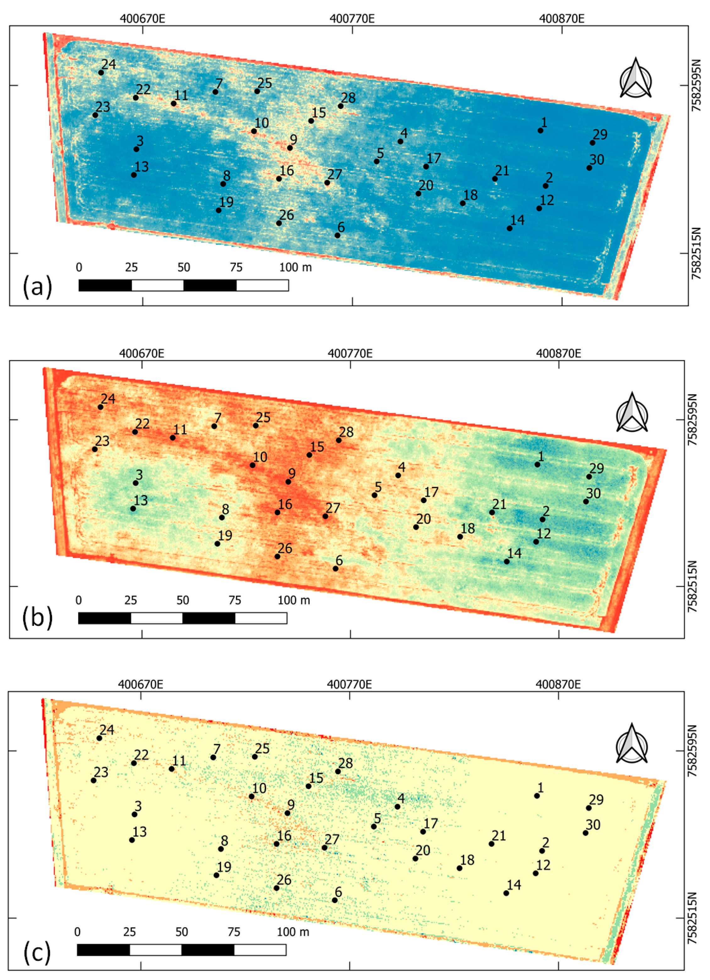
Figure 6 shows a coloured representation generated for NDVI, SR, and TCARI using uniform slicing of the data range to form classes. We hypothesise that these vegetative vigour classes have a relation with soybean yield. Based on these classes, a set of 30 sample plots was defined based on the variability identified in those spectral indices. A similar number of samples for each class will ensure representative and balanced data for all classes. As can be observed, NDVI (Figure 6a) indicates areas of higher and lower vegetative vigour, but its capacity to identify local variability is lower when compared to SR (Figure 6b). The latter makes it feasible to highlight the differences. Then, the sampling process can be better conducted to capture the heterogeneity of the area using the indices as a priori knowledge. The TCARI (Figure 6c) shows lower variability in the canopy of the soybean plantation, indicating that indices associated with vegetation vigour are more significant for selecting sample points.
The vegetation indices and absolute heights were derived from the orthomosaics and CHM, respectively. All 25 bands from the hyperspectral sensor (registered orthomosaics) were used to extract the digital number from the pixels. Sequentially, the hyperspectral data were used to compute the six vegetation indices (in Table 4). A polygon-shaped shapefile was used to delineate the area of interest in all image layers and guide the extraction of attributes in QGIS software (version 3.4 open-source, Raleigh, NC, USA) using a point sampling tool. The attributes were associated with each pixel in the layer stack to be used in the machine learning algorithms. The pixels referring to the sample plots were related to the data collected in the field to be used in the productivity prediction models. These data were used to train and test the algorithms.

2.2.4. Crop Sample Collection

Stratified random sampling [36] was used to conduct the selection of spatial sample plots relying on spectral reference. Since the spectral response is correlated with plant vigour, there is an expectation that the variability of biophysical parameters is associated with specific subareas. Therefore, stratified random sampling can contribute to biophysical parameterisation purposes, enabling a sampling strategy based on multiple subgroups (or strata) within the area. Randomness occurs within each stratum, which allows each subgroup to be represented by one or more samples. In areas with low variability (spectrally homogenous), the distribution of random points ensures the collection of representative samples. In contrast, variability is not guaranteed in heterogeneous areas by using only random samples unless very-high-density sampling is performed at a very high cost. Instead, using a priori information evidenced by spectral indices can contribute to selecting sample plots with higher confidence at a reasonable cost. Vegetation indices are usually adopted to evaluate vegetation vigour and health. Therefore, homogeneous regions of vegetation index values can be extracted, and samples are selected in each region randomly. This approach is a spatial application of the stratified random sampling process.
The image blocks were georeferenced by photogrammetric processing to obtain high-precision geodetic coordinates. Thus, from the points selected in the vegetation indices, each coordinate was located in the field using an RTK (Real Time Kinematic) GNSS receiver (Topcon Positioning System, Inc., Livermore, CA, USA) with 5 cm accuracy in kinematic mode. At harvest time, an area of 5 m2 (4 planting lines with a length of 2.5 m) around each point was considered to collect all plants within that area for counting, weighing, height measurement, and productivity estimation. The data collected in the sampling plots were proportionally converted to a 50 cm grid in the information layers. The purpose was to obtain the local variability from samples collected in situ. Then, the sample variability could be associated with image feature variations to estimate productivity based on predictive machine learning algorithms such as RF and multiple linear regression (MLR).
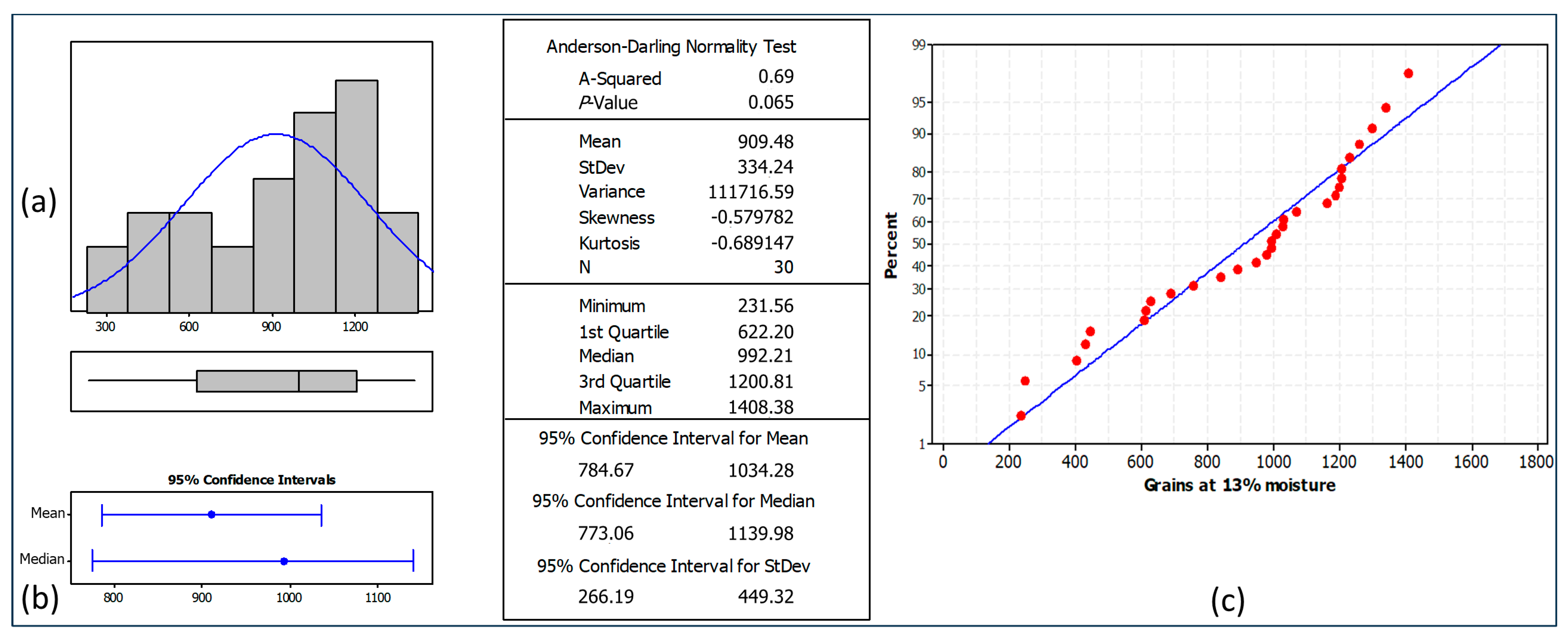
The soybean samples were weighted within each plot. The wet mass was weighed, and after the drying procedure, it was compared to the dry mass to obtain the net weight of grains with correction for the reference of 13% moisture. As 13% of the weight is water, the other 87% is dry mass. Figure 7a presents descriptive statistics of the sample results, calculated in Minitab statistical software version 17 (Minitab Statistical Software, State College, PA, USA), in which the histogram with data grouped in intervals can be observed, with the normal curve as reference. The resulting values are between 231.56 g and 1408.38 g, with an average of 909.48 g and a standard deviation of 334.24 g. The boxplot shows a slight asymmetry and indicates the median at 992.21 g. Considering the 95% confidence interval for the median (Figure 7b), the values appear between 773.06 g and 1139.98 g. No outlier was detected in the sample set. The Anderson–Darling normality test was applied to verify the fit of the data to the normal distribution at a significance level of 5%. As a result, the statistical test obtained a p-value (0.065) > 0.05, indicating no evidence to reject the assumption of normality. Therefore, we can consider the data to be close to the normal distribution (Figure 5a,c).
From the net weight of grains at 13% moisture, the local grain yield was calculated with respect to the sample plot area (kg/m2) and then converted to kg/ha. Figure 8 shows the result of local productivity in each one of the sample plots. Yield variability can be observed and considered when calculating soybean yield estimates for the entire area. The predictor models must capture this variability, and then a more accurate estimate can be produced with the remote sensing data.

2.2.5. Prediction Models

The estimation process used in the experiments is based on the RF and MLR algorithms. The RF technique was introduced by Breiman [37] and has been widely used as a predictive or regressive model for different remote sensing problems. Previous studies [38,39] have shown that RF is not influenced by irrelevant predictors, and variable reduction does not have a significant impact on technical performance. The RF algorithm implemented in Weka Software, version 3.8.1 (Campbell, New Zealand), was used in this approach for feature selection and validation, resulting in one of the prediction models. The number of decision trees was set to 100, and other parameters were used in their default mode: maximum number of features for each split = n u m b e r   o f   f e a t u r e s ; minimum number of samples for leaf nodes = 1; minimum number of samples for splitting internal nodes = 2; and number of randomly chosen attributes = int(log_2(number of predictors) + 1).
The MLR technique estimates model parameters using the relationship between two or more independent variables and a response variable by adjusting a linear equation to the observed data, usually calculated using the least-squares method. The implementation available in Weka (v. 3.8.1) was also used in this task. The selection of the characteristic model was based on the M5 method, which is a backward elimination method in which the feature with the lowest standardised coefficient is removed until no improvement is observed in the Akaike information criterion [40].
The performance of linear regression is usually poor when there are highly correlated input features. Thus, the MLR algorithm in the Weka software was configured to eliminate collinear features and select the most relevant uncorrelated features. The Akaike information criterion [40], used in the algorithm, tests how the inclusion and/or exclusion of variables improves the fit of the data in modelling. It also allows comparison between models since the criterion only depends on the sum of squares of the residuals rather than the sample size.
The grain yield measurement collected in situ was defined as the dependent variable of the predictive algorithms. The spectral reflectance of the 25 hyperspectral bands and the six vegetation indices were used as predictive variables. The average height was also tested as a predictive variable. In the images, it was considered a 3 × 3 pixel window around each sample plot, representing grain productivity proportional to its area. Thus, each plot was used to adjust the model with 9 observations (3 × 3 pixels), which generated a set of 30 × 9 = 270 observations to be tested in the machine learning algorithms. K-fold cross-validation was used to assess the estimates by predictive algorithms to ensure that the training and test data were independent between runs. This technique divides the dataset into a k number of folds and has been considered to be superior to split-sample techniques, mainly in small datasets, according to Drummond et al. [41]. In this study, the dataset was divided into 80% for training and 20% for testing.

2.3. Performance Assessment

The algorithmic performance of models based on different algorithms, trained with different datasets, was measured using Pearson’s correlation coefficient (r), mean absolute error (MAE), root mean square error (RMSE), relative absolute error (RAE), and root relative squared error (RRSE). Such measures were calculated on the randomised 10-fold cross-validation for both machine learning algorithms.
The best-adjusted prediction model was applied to images, and a productivity map was produced to show the spatial distribution of the grain yield. The sum of the pixel values provides an estimated mass of grains (kg) in the area (ha). For validation, the weight of the harvested soybean was used as a reference in the accuracy analysis of the estimates. The estimate based on remote sensing data was compared with the harvest’s net weight to assess the techniques’ accuracy. To assess the accuracy of the prediction models, the sum of the pixel values in the yield map provides the grain mass yield value at 13% moisture (net weight in kg).

3. Results

3.1. Machine Learning Estimators for Soybean Yield Productivity

Table 5 presents the results of the MLR algorithm produced with several sets of attributes using 270 instances. The purpose was to analyse the contribution of each attribute to estimate soybean grain productivity by considering productivity as a response variable. The “Most significant features” column presents, in descending order, the sequence of the features selected by the algorithm according to the input dataset. When all 25 hyperspectral bands were used, only 13 of them were significant, in which the three most important bands were 25 (829 nm), 22 (771 nm), and 23 (790 nm), located in the near-infrared region, while the three least important bands were 7 (591 nm), 5 (566 nm), and 4 (552 nm) located in the green region. The resulting correlation coefficient was r = 0.77 and did not change when the “height” feature was included, indicating that the vertical structure had a low contribution in improving the model’s fitting. However, the RAE and RRSE values showed a slight reduction. Using only the “six indices” as predictor variables caused an increase in the correlation coefficient to r = 0.79. The SAVI was the most significant in this case, while the NDVI was discarded. Adding “height” to the set of indices also did not add significant improvements since the previous results did not change, but a slight reduction in the RAE and RRSE was observed.
Another test was carried out by considering the attributes “25 bands + 6 indices” together and then adding the height (25 bands + 6 indices + height) to identify the most significant features. As a result, the features of the hyperspectral bands were more significant than the vegetation indices since they were prior to the indices in the sequence of the MLR adjustment. However, the value of r = 0.79 was similar to the result when only the six indices were used, demonstrating that the vegetation indices (derived from only four bands) may be sufficient to capture the main spectral information related to soybean productivity. The height feature was not relevant to the result. In all six sets analysed, the values of MAE and RMSE were similar.
The previous analysis showed that the adjusted MLR model achieved R2 = 0.62 in the best case, indicating that the features used can explain 62% of the response variable (productivity). The RF algorithm was applied for comparison purposes to produce a nonlinear regression model since it is based on binary trees and calculates the predictions using all tree data. The same five datasets used for MLR were tested with the RF algorithm to assess the correction coefficient and the resulting errors. Table 6 presents the results using randomised cross-validation with k = 10 folds and 10 repetitions. The lowest correlation coefficient (r = 0.83) was obtained when only the 25 bands were used as attributes. However, introducing the height feature to the RF model performance significantly increased the correlation coefficient to r = 0.89 and reduced the percentages of RAE and RRSE by more than 8%.
Considering only the six indices as features, r = 0.81 was obtained, and it was improved to r = 0.88 when the height feature was included in the dataset, reducing RAE and RRSE by more than 10%. The simultaneous use of the “25 bands + 6 indices” values generated an r = 0.84, which was increased to r = 0.88 by including the height feature. In all cases, the structural variable “height” contributed significantly to improving the fit of the RF regressive algorithm.
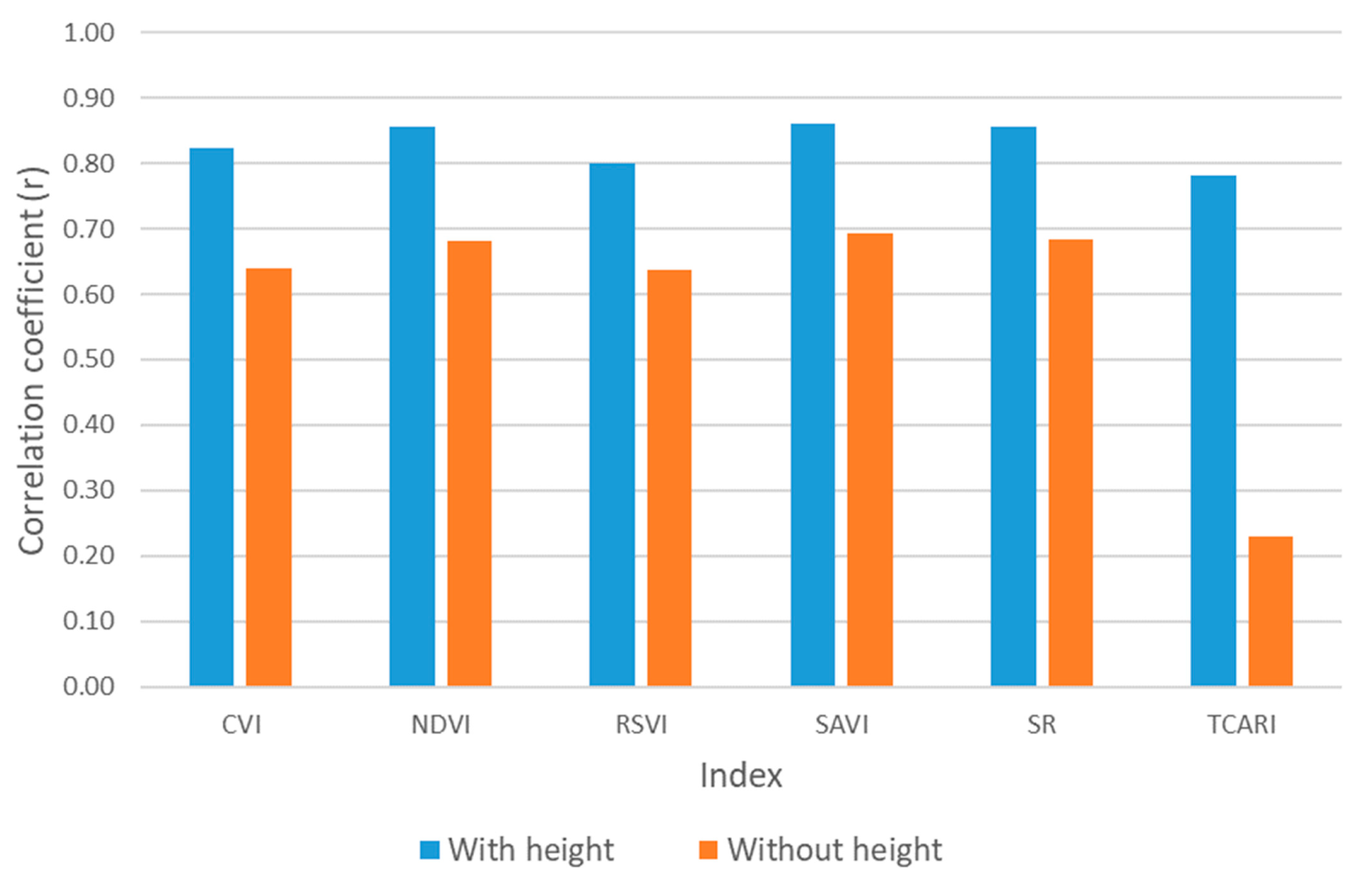
To analyse the potential of the six indices in the productivity estimation, each index was tested in the RF together. The height feature was also tested to assess its contribution to the prediction model. Figure 9 shows the correlation coefficient for the six vegetation indices. When the height feature was not used, the values of r were below r = 0.7. It should be noted that the TCARI (r = 0.23) showed the most discrepant value compared to the other indices.
On the other hand, the height inclusion as a feature in the model increased all r values to the range [0.78–0.86], with the highest value (r = 0.86) obtained with NDVI, SAVI, and SR. In all cases, MAE and RMSE were equal to 0.01. The results also demonstrate that the combined use of indices improves the estimates, which was also reported by Zhao et al. [9] in the prediction of field-scale wheat yield.
Since tests with the MLR model demonstrated that the contribution of the spectral bands was more significant than the contribution of the indices, additional experiments with RF were conducted using four spectral bands (see Section 2.2.3) used for sample selection along with the attributes of NDVI, SR, and height. Table 7 shows the results of the RF models fitted with different datasets by combining the four bands with the two indices and height. When only the four bands were used, r = 0.84 was obtained, and including the two indices produced a lower r = 0.83. The addition of height in the model significantly increased the correlation coefficient to r ≥ 0.90. The values of MAE and RMSE were similar in all tests. Comparing the results, the best model adjusted with RF was achieved using four bands with heights. This combination of attributes resulted in the highest value of r and lowest percentages of RAE (35.13%) and RRSE (40.96%). It is worth mentioning that the four bands selected are commonly found in orbital multispectral sensors.

3.2. Soybean Productivity Map and Validation

From the results presented in the previous sections, the combination of the features “4 bands + height” was selected to adjust the RF regression model to predict soybean yield. So, the adjusted model was applied to images to produce a productivity map, as shown in Figure 10a. A prediction map was also created with the best model adjusted by the MLR algorithm (Figure 10b), using the attributes “25 bands + 6 indices + height” evaluated in Table 5. The objective was to enable a spatial comparison between both estimates.
Both maps represent the soybean productivity in kg per pixel and are presented following a classification, considering equal intervals with five classes. As shown in Figure 10a, the RF model indicates the local productivity potential with greater emphasis, in which the blue colour represents higher productivity. In contrast, the MLR shows a smoother result (Figure 10b), concentrating the values from 0.064 to 0.021 kg/pixel. Both models are consistent with the characteristics surveyed in the field and reflect the local variability identified in the study area.
Table 8 compares the estimated results concerning the net weight of the harvested grains (reference data) and the productivity per hectare. The first comparison was carried out between the sample mean directly calculated on the plot data, which indicated a difference of 3.1% in relation to the reference weight. The productivity estimated with the MLR model achieved a difference of 2.8%, while the RF model produced the best result, presenting a difference of 1.5%.

4. Discussion

This study investigated soybean grain yield estimation using UAV-based hyperspectral imaging and photogrammetric 3D modelling. Two machine learning regression techniques (MLR and RF) were used to produce estimates from in situ data. The cross-validation was used with ten folds, resulting in an average bias of 1.20% for MLR and -0.47% for RF.
Significant accuracies were achieved due to the sampling procedure guided by evidence of spectral variability detected from image data and by applying a sample delineation technique, which allows the selection of random samples in a stratified dataset. This finding is essential to demonstrate that the spectral response of soybeans in the reproductive stage is related to productivity and can be captured by remote sensing techniques. There was an initial concern about whether the stratified random sampling could lead to biased results. However, the definition of the sample plot locations was determined by spectral evidence, in which three vegetation indices were adopted with slicing at class intervals, allowing the selection of representative elements of each class. Furthermore, the features derived from high-resolution imagery showed that spectral information combined with the vertical structure (height) significantly contributed to estimating the soybean productivity when the model was fitted using the RF algorithm. The model was also able to adjust to a condition of large dispersion of the effect of soil attributes on soybean yield due to the distribution of coefficients found by the multiple regression model applied.
The experiments demonstrated that adding height to the prediction model can produce better results, depending on the machine learning algorithm. For the MLR algorithm, the height attribute did not significantly improve the estimates, likely because the vertical structure is correlated with the spectral bands close to the R and IR bands (the estimate without height produced an r = 0.77, and with height, it was r = 0.79). In contrast, the nonlinear regression model, fitted by the RF algorithm, showed better performance when using the height features (the estimate without height produced an r = 0.83, and with the height, it was r = 0.89, considering 25 bands and height). Thus, as noted by other studies (e.g., [5,12,19,42]), regressive models based on trees are more suitable for estimating productivity. Furthermore, in this study, instead of using the information of only one pixel, the size of each sample area was composed of nine pixels with productivity values proportional to the spatial dimension. Thus, each set of sample pixels allowed an increase in the number of local features for the various information layers, representing the variation in plant productivity.
In general, the experiments showed that a set with many spectral bands was not necessary. In the MLR algorithm, indices with some bands can be used rather than considering multiple bands. On the other hand, the nonlinear RF algorithm performed better with spectral bands along with the height attribute and was significantly superior to the MLR algorithm in estimating productivity. The results showed that using four spectral bands (552 nm, 672 nm, 701 nm, 810 nm) together with the height attribute produced a better result (r = 0.91) in the RF prediction model, which indicated an R2 = 0.828. It is worth highlighting that two of these bands are in the red-edge region, which are not easily found in multispectral sensors. The results obtained in this study were higher than the R2 = 0.70 reached by Wei and Molin [3] to estimate soybean yield considering the number of grains and thousand-grain weight in a linear regression approach. The R2 found in this research was similar to the value R2 = 0.824 obtained by Maimaitijiang et al. [5] using a deep neural network with different types of images (multispectral, thermal, and RGB) in rainfed soybean. It is worth mentioning that machine learning approaches such as RF require a significantly lower sample number than deep learning algorithms. The experiments conducted by Eugenio et al. [14] with multispectral images and machine learning resulted in R2 = 0.84. However, soybean yield estimates were carried out on irrigated soybean crops, that is, in a controlled area, while the approach studied in this research was developed with a rainfed soybean crop. The RF model demonstrated a better ability to identify and estimate the production potential within the study area, compared to the MLR model. The estimated value was compared with the weight of grains harvested at 13% moisture to obtain an accuracy measure. The difference between the estimated and collected weights was 1.5% in this case study.
Another relevant issue for more accurate modelling is the representativity of the samples. Traditional methods of soybean yield determination use flow meters in harvesters. Although this approach is the most precise method, it is performed only at the end of the harvest. Our proposal for sampling design aims to minimise the bias and obtain statistically representative samples of the spatial variation in soybean yield. Due to the data augmentation technique applied, a significant number of samples were obtained, resulting in a satisfactory performance of the soybean prediction model. The plant growth stage also has an important role in model accuracy. The area of interest is located in a region where the rainfall regime is very irregular. In drier years, the soybean development and the process of ageing are accelerated, affecting the development of the pods and seed grain. In addition, heat waves also cause the abortion of flowers. Other factors also affecting the productivity are the type of soil, soil compactness, and nematodes. Therefore, adopting the R5 stage seems adequate because the vegetation has already undergone the stress caused by external factors, having more correlation with the final productivity.

5. Conclusions

We investigated the spatial and spectral variability in soybean canopy reflectance, aiming for grain yield estimation. High-resolution hyperspectral images were used within the 500–900 nm continuous spectrum (in 25 bands) to evaluate the spectral bands and derive vegetation spectral indices. RF and MLR machine learning algorithms were used following spectral evidence, which allowed for successful productivity estimation. Traditional methods of sampling design do not guarantee that the samples represent all the variability of the variables of interest and have samples balanced to each class. Hence, the method proposed sought to cover all the variability of the independent variable based on the spatial distribution of the spectral variability observed in vegetation spectral indices. Applying the methodology in a study area with local variability enabled an assessment of the sampling technique based on spectral evidence as a priori knowledge to collect samples for prediction models. The proposed technique of data augmentation allowed a significant increase in the number of instances for modelling.
In the multivariate regression models with RF and MLR, all independent variables were derived from remote sensing data, which showed that they could generate soybean productivity models. The height features extracted from the DSM contributed significantly to the RF prediction model but did not impact MLR estimates. The sampling procedure efficiently captured the variability in vegetation vigour in the R5 growth stage, which indicated a correlation with productivity. Thus, a more accurate productivity prediction was produced by considering this variability in the regression model. Once again, RF proved to be robust when there is redundant information among features, resulting in satisfactory performance using 25 spectral bands. This study aimed to analyse the continuous spectrum of the hyperspectral bands (narrow bands) and the selection of samples based on the spectral response (combination of soil and vegetation) to estimate soybean productivity. In future work, the productivity prediction model should be evaluated in places with other characteristics, larger-bandwidth multispectral sensors, and other spatial image resolutions. The adjusted models will also be applied to other study areas to assess the adherence of the models for the extrapolation of estimates and the workable number of samples to ensure efficiency for prediction.

Author Contributions

Conceptualization, methodology, writing: A.B. and N.N.I.; data curation, writing—original draft preparation: F.S.Y.W.; reviewing, original draft preparation: A.M.G.T.; writing, editing: G.M.P.E.; data curation, writing—original draft preparation: F.F.d.A.; data curation and validation: G.C.L.; writing–review and investigation: E.H. All authors have read and agreed to the published version of the manuscript.

Funding

This research was funded by the São Paulo Research Foundation FAPESP (2021/06029-7, 2021/10823-0), the National Council for Scientific and Technological Development CNPq (Grants: 303670/2018-5, 308747/2021-6) and the Coordenação de Aperfeiçoamento de Pessoal de Nível Superior (CAPES) (Code 88887.310313/2018-00 and 88881.310314/2018-01).

Data Availability Statement

Data will be made available on request.

Conflicts of Interest

The authors declare no conflicts of interest.

References

  1. USDA (United States Department of Agriculture) World Agricultural Production; Foreign Agricultural Service. Circular Series WAP 2-20: USA. 2020. Available online: https://apps.fas.usda.gov/PSDOnline/Circulars/2020/02/production.pdf (accessed on 2 September 2024).
  2. da Silva, E.E.; Baio, F.H.R.; Teodoro, L.P.R.; da Silva, C.A., Jr.; Borges, R.S.; Teodoro, P.E. UAV-Multispectral and Vegetation Indices in Soybean Grain Yield Prediction Based on in Situ Observation. Remote Sens. Appl. Soc. Environ. 2020, 18, 100318. [Google Scholar] [CrossRef]
  3. Wei, M.C.F.; Molin, J.P. Soybean Yield Estimation and Its Components: A Linear Regression Approach. Agriculture 2020, 10, 348. [Google Scholar] [CrossRef]
  4. Banerjee, B.P.; Spangenberg, G.; Kant, S. Fusion of Spectral and Structural Information from Aerial Images for Improved Biomass Estimation. Remote Sens. 2020, 12, 3164. [Google Scholar] [CrossRef]
  5. Maimaitijiang, M.; Sagan, V.; Sidike, P.; Hartling, S.; Esposito, F.; Fritschi, F.B. Soybean Yield Prediction from UAV Using Multimodal Data Fusion and Deep Learning. Remote Sens. Environ. 2020, 237, 111599. [Google Scholar] [CrossRef]
  6. Parmley, K.A.; Higgins, R.H.; Ganapathysubramanian, B.; Sarkar, S.; Singh, A.K. Machine Learning Approach for Prescriptive Plant Breeding. Sci. Rep. 2019, 9, 17132. [Google Scholar] [CrossRef]
  7. de Siqueira, D.A.B.; Vaz, C.M.P.; da Silva, F.S.; Ferreira, E.J.; Speranza, E.A.; Franchini, J.C.; Galbieri, R.; Belot, J.L.; de Souza, M.; Perina, F.J.; et al. Estimating Cotton Yield in the Brazilian Cerrado Using Linear Regression Models from MODIS Vegetation Index Time Series. AgriEngineering 2024, 6, 947–961. [Google Scholar] [CrossRef]
  8. Wang, Y.; Zhang, Z.; Feng, L.; Du, Q.; Runge, T. Combining Multi-Source Data and Machine Learning Approaches to Predict Winter Wheat Yield in the Conterminous United States. Remote Sens. 2020, 12, 1232. [Google Scholar] [CrossRef]
  9. Zhao, Y.; Potgieter, A.B.; Zhang, M.; Wu, B.; Hammer, G.L. Predicting Wheat Yield at the Field Scale by Combining High-Resolution Sentinel-2 Satellite Imagery and Crop Modelling. Remote Sens. 2020, 12, 1024. [Google Scholar] [CrossRef]
  10. Gumma, M.K.; Nukala, R.M.; Panjala, P.; Bellam, P.K.; Gajjala, S.; Dubey, S.K.; Sehgal, V.K.; Mohammed, I.; Deevi, K.C. Optimizing Crop Yield Estimation through Geospatial Technology: A Comparative Analysis of a Semi-Physical Model, Crop Simulation, and Machine Learning Algorithms. AgriEngineering 2024, 6, 786–802. [Google Scholar] [CrossRef]
  11. Gao, F.; Anderson, M.; Daughtry, C.; Karnieli, A.; Hively, D.; Kustas, W. A Within-Season Approach for Detecting Early Growth Stages in Corn and Soybean Using High Temporal and Spatial Resolution Imagery. Remote Sens. Environ. 2020, 242, 111752. [Google Scholar] [CrossRef]
  12. Ramos, A.P.M.; Osco, L.P.; Furuya, D.E.G.; Gonçalves, W.N.; Santana, D.C.; Teodoro, L.P.R.; da Silva, C.A., Jr.; Capristo-Silva, G.F.; Li, J.; Baio, F.H.R.; et al. A Random Forest Ranking Approach to Predict Yield in Maize with Uav-Based Vegetation Spectral Indices. Comput. Electron. Agric. 2020, 178, 105791. [Google Scholar] [CrossRef]
  13. dos Silva, F.D.S.; Peixoto, I.C.; Costa, R.L.; Gomes, H.B.; Gomes, H.B.; Cabral Júnior, J.B.; de Araújo, R.M.; Herdies, D.L. Predictive Potential of Maize Yield in the Mesoregions of Northeast Brazil. AgriEngineering 2024, 6, 881–907. [Google Scholar] [CrossRef]
  14. Eugenio, F.C.; Grohs, M.; Venancio, L.P.; Schuh, M.; Bottega, E.L.; Ruoso, R.; Schons, C.; Mallmann, C.L.; Badin, T.L.; Fernandes, P. Estimation of Soybean Yield from Machine Learning Techniques and Multispectral RPAS Imagery. Remote Sens. Appl. Soc. Environ. 2020, 20, 100397. [Google Scholar] [CrossRef]
  15. Zhang, X.; Zhao, J.; Yang, G.; Liu, J.; Cao, J.; Li, C.; Zhao, X.; Gai, J. Establishment of Plot-Yield Prediction Models in Soy-bean Breeding Programs Using UAV-Based Hyperspectral Remote Sensing. Remote Sens. 2019, 11, 2752. [Google Scholar] [CrossRef]
  16. de Queiroz Otone, J.D.; de Theodoro, G.F.; Santana, D.C.; Teodoro, L.P.R.; de Oliveira, J.T.; de Oliveira, I.C.; da Silva Junior, C.A.; Teodoro, P.E.; Baio, F.H.R. Hyperspectral Response of the Soybean Crop as a Function of Target Spot (Corynespora Cassi-icola) Using Machine Learning to Classify Severity Levels. AgriEngineering 2024, 6, 330–343. [Google Scholar] [CrossRef]
  17. Fehr, W.R.; Caviness, C.E. Stages of Soybean Development; Iowa State University of Science and Technology: Ames, IA, USA, 1977; Volume 87. [Google Scholar]
  18. Ma, B.L.; Dwyer, L.M.; Costa, C.; Cober, E.R.; Morrison, M.J. Early Prediction of Soybean Yield from Canopy Reflectance Measurements. Agron. J. 2001, 93, 1227–1234. [Google Scholar] [CrossRef]
  19. Luo, S.; Liu, W.; Zhang, Y.; Wang, C.; Xi, X.; Nie, S.; Ma, D.; Lin, Y.; Zhou, G. Maize and Soybean Heights Estimation from Unmanned Aerial Vehicle (UAV) LiDAR Data. Comput. Electron. Agric. 2021, 182, 106005. [Google Scholar] [CrossRef]
  20. Bendig, J.; Yu, K.; Aasen, H.; Bolten, A.; Bennertz, S.; Broscheit, J.; Gnyp, M.L.; Bareth, G. Combining UAV-Based Plant Height from Crop Surface Models, Visible, and near Infrared Vegetation Indices for Biomass Monitoring in Barley. Int. J. Appl. Earth Obs. Geoinf. 2015, 39, 79–87. [Google Scholar] [CrossRef]
  21. Geipel, J.; Link, J.; Claupein, W. Combined Spectral and Spatial Modeling of Corn Yield Based on Aerial Images and Crop Surface Models Acquired with an Unmanned Aircraft System. Remote Sens. 2014, 6, 10335–10355. [Google Scholar] [CrossRef]
  22. Yin, X.; McClure, M.A.; Jaja, N.; Tyler, D.D.; Hayes, R.M. In-Season Prediction of Corn Yield Using Plant Height under Major Production Systems. Agron. J. 2011, 103, 923–929. [Google Scholar] [CrossRef]
  23. Yu, N.; Li, L.; Schmitz, N.; Tian, L.F.; Greenberg, J.A.; Diers, B.W. Development of Methods to Improve Soybean Yield Estimation and Predict Plant Maturity with an Unmanned Aerial Vehicle Based Platform. Remote Sens. Environ. 2016, 187, 91–101. [Google Scholar] [CrossRef]
  24. Senop Ltd. Available online: http://senop.fi/en/optronics-hyperspectral (accessed on 20 October 2018).
  25. Oliveira, R.A.; Tommaselli, A.M.G.; Honkavaara, E. Geometric Calibration of a Hyperspectral Frame Camera. Photogramm. Rec. 2016, 31, 325–347. [Google Scholar] [CrossRef]
  26. Tommaselli, A.M.G.; Santos, L.D.; Oliveira, R.A.; Berveglieri, A.; Imai, N.N.; Honkavaara, E. Refining the Interior Orienta-tion of a Hyperspectral Frame Camera with Preliminary Bands Co-Registration. IEEE J. Sel. Top. Appl. Earth Obs. Remote Sens. 2019, 12, 2097–2106. [Google Scholar] [CrossRef]
  27. Berveglieri, A.; Tommaselli, A.M.G.; Santos, L.D.; Honkavaara, E. Bundle Adjustment of a Time-Sequential Spectral Cam-era Using Polynomial Models. IEEE Trans. Geosci. Remote Sens. 2019, 57, 9252–9263. [Google Scholar] [CrossRef]
  28. Rapidlasso GmbH. LAStools—Fast Tools to Catch Reality. Available online: http://rapidlasso.com/LAStools (accessed on 4 March 2020).
  29. Patrício, D.I.; Rieder, R. Computer Vision and Artificial Intelligence in Precision Agriculture for Grain Crops: A Systematic Review. Comput. Electron. Agric. 2018, 153, 69–81. [Google Scholar] [CrossRef]
  30. Rouse, J.W., Jr.; Haas, R.H.; Schell, J.A.; Deering, D.W. Monitoring Vegetation Systems in the Great Plains with Erts; NASA Special Publication: Washington, DC, USA, 1974; Volume 351, p. 309.
  31. Jordan, C.F. Derivation of Leaf-Area Index from Quality of Light on the Forest Floor. Ecology 1969, 50, 663–666. [Google Scholar] [CrossRef]
  32. Haboudane, D.; Miller, J.R.; Tremblay, N.; Zarco-Tejada, P.J.; Dextraze, L. Integrated Narrow-Band Vegetation Indices for Prediction of Crop Chlorophyll Content for Application to Precision Agriculture. Remote Sens. Environ. 2002, 81, 416–426. [Google Scholar] [CrossRef]
  33. Huete, A.R. A Soil-Adjusted Vegetation Index (SAVI). Remote Sens. Environ. 1988, 25, 295–309. [Google Scholar] [CrossRef]
  34. Merton, R. Monitoring Community Hysteresis Using Spectral Shift Analysis and the Red-Edge Vegetation Stress Index. In Proceedings of the Seventh Annual JPL Airborne Earth Science Workshop, Pasadena, CA, USA, 12–16 January 1998; JPL: Pasadena, CA, USA, 1998; pp. 12–16. [Google Scholar]
  35. Vincini, M.; Frazzi, E.; D’Alessio, P. A Broad-Band Leaf Chlorophyll Vegetation Index at the Canopy Scale. Precis. Agricult. 2008, 9, 303–319. [Google Scholar] [CrossRef]
  36. Larson, R.; Farber, B. Elementary Statistics: Picturing the World, 6th ed.; Pearson Education, Inc.: Boston, MA, USA, 2015. [Google Scholar]
  37. Breiman, L. Random Forests. Mach. Learn. 2001, 45, 5–32. [Google Scholar] [CrossRef]
  38. Heung, B.; Bulmer, C.E.; Schmidt, M.G. Predictive Soil Parent Material Mapping at a Regional-Scale: A Random Forest Approach. Geoderma 2014, 214–215, 141–154. [Google Scholar] [CrossRef]
  39. Li, Z.; Xin, X.; Tang, H.; Yang, F.; Chen, B.; Zhang, B. Estimating Grassland LAI Using the Random Forests Approach and Landsat Imagery in the Meadow Steppe of Hulunber, China. J. Integr. Agric. 2017, 16, 286–297. [Google Scholar] [CrossRef]
  40. Akaike, H. A New Look at the Statistical Model Identification. IEEE Trans. Autom. Control 1974, 19, 716–723. [Google Scholar] [CrossRef]
  41. Drummond, S.T.; Sudduth, K.A.; Joshi, A.; Birrell, S.J.; Kitchen, N.R. Statistical and Neural Methods for Site–Specific Yield Prediction. Trans. ASAE 2003, 46, 5. [Google Scholar] [CrossRef]
  42. Lee, H.; Wang, J.; Leblon, B. Using Linear Regression, Random Forests, and Support Vector Machine with Unmanned Aeri-al Vehicle Multispectral Images to Predict Canopy Nitrogen Weight in Corn. Remote Sens. 2020, 12, 2071. [Google Scholar] [CrossRef]
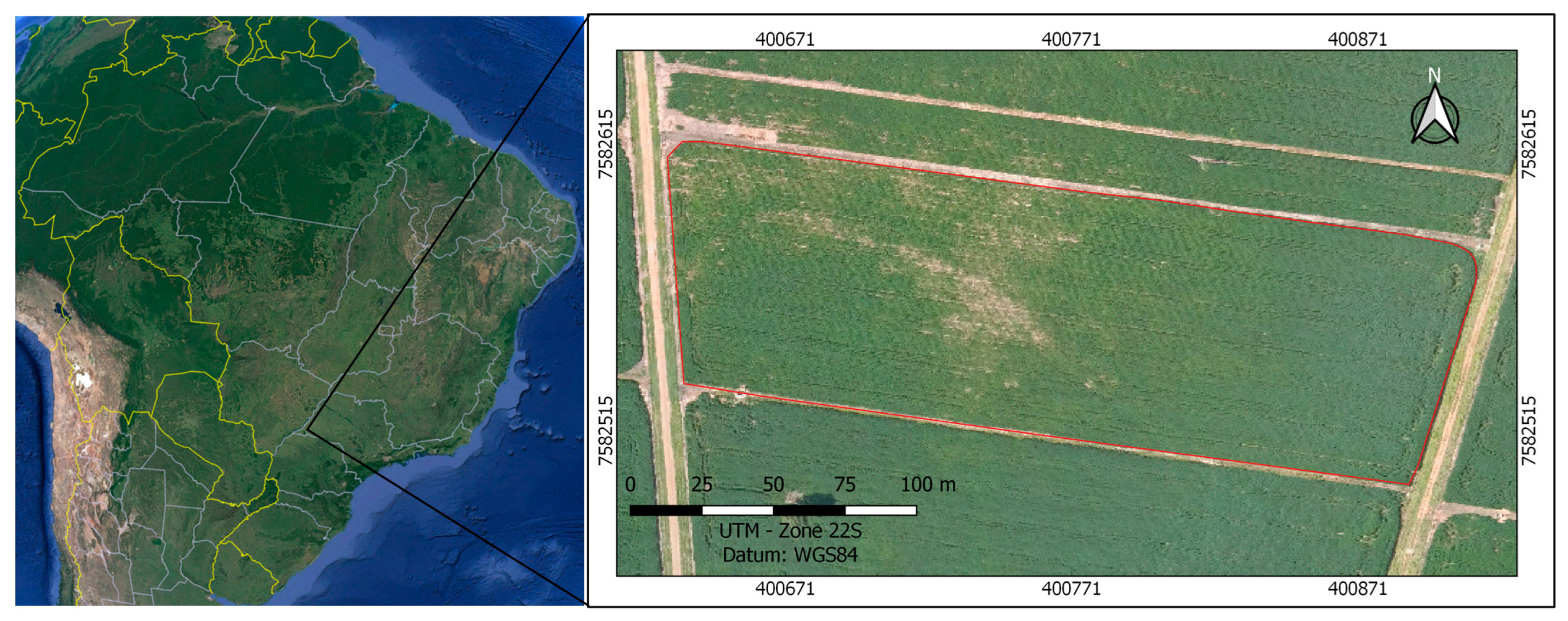
Figure 1. Study area with soybean planting delimited by the red line—located in the western region of the state of São Paulo, Brazil. Image sources: Google Earth (on the left) and RGB image collected on 25 January 2020, with a UAV Phantom 3—DJI (on the right).
Agriengineering 06 00185 g001
Figure 2. Timeline presenting the progress of data collection in the study area.
Agriengineering 06 00185 g002
Figure 3. (a) FPI camera; (b) UAV in operation to acquire hyperspectral images.
Agriengineering 06 00185 g003
Figure 4. Image block adjustment of a hyperspectral band, showing two flying strips and six GCPs.
Agriengineering 06 00185 g004
Figure 5. (a) DTM. (b) Example of a cross-section in the CHM.
Agriengineering 06 00185 g005
Figure 6. Positions selected for 30 sample plots following the variability evidenced by the spectral indices: (a) NDVI; (b) SR; and (c) TCARI.
Agriengineering 06 00185 g006
Figure 7. (a) Descriptive statistics; (b) confidence interval; (c) normality test chart (red dots are the observed values).
Agriengineering 06 00185 g007
Figure 8. Grain yield production in kg/ha estimated from each sample plot, following the spatial distribution of Figure 6.
Agriengineering 06 00185 g008
Figure 9. Comparison of results with the RF model when the height attribute is used with each vegetation index.
Agriengineering 06 00185 g009
Figure 10. Maps of grain productivity generated by the predictor models: (a) RF and (b) MLR.
Agriengineering 06 00185 g010
Table 1. Technical details of the hyperspectral camera (Senop Ltd., Finland) [24].
DescriptionSpecification
Camera modelRikola FPI2015
Nominal focal length9 mm
Pixel size5.5 μm
Image size1017 × 648 pixels
Sensors2 CMOS
Spectral range500–900 nm (spectral step 1 nm)
Spectral resolution10 nm—FWHM (full width at half maximum)
Weight<700 g
Table 2. Spectral band configuration of Rikola FPI2015 camera.
1st Sensor2nd Sensor
Band Positionλ (nm)Band Positionλ (nm)
1509.3511654.21
2522.4712663.02
3538.1213672.61
4552.9114684.10
5566.2915691.90
6581.3316701.27
7591.9017712.06
8606.3618723.16
9620.2219731.22
10633.4120741.37
21751.06
22771.87
23790.30
24810.46
25829.39
Table 3. Aerial survey configuration with the FPI camera.
ParameterFPI Camera
Flying height160 m
Forward and side overlap80% and 60%
Number of flying strips2
Flying speed4 m/s
Integration time5 ms
Table 4. Vegetation indices derived from the hyperspectral image cube and used as attributes for the machine learning model, according to the ranges green (G), red (R), red-edge (RE) and near-infrared (NIR).
Vegetation IndexFull FormFormulation with the Adopted BandsReference
NDVINormalised difference vegetation index(NIR810 − R672)/(NIR810 + R672)[30]
SRSimple ratio indexNIR810/R672[31]
TCARITransformed chlorophyll absorption in the reflectance index3 × [(RE701−R672) − 0.2(RE701−G552) × (RE701/R672)][32]
SAVISoil-adjusted vegetation index(NIR810 − R672)/(NIR810 + R672 + 0.5) × (1 + 0.5)[33]
RSVIRed-edge stress vegetation index[(RE723 + RE751)/2] − RE731[34]
CVIChlorophyll vegetation indexNIR829 × [R663/(G566)2][35]
Table 5. Results with the MLR algorithm using six datasets of attributes as predictor variables.
Predictor VariablesMost Significant Attributes
(in Descending Order) *
rMAERMSERAE (%)RRSE (%)
25 bands25 22 23 17 15 14 12 11 9 8 7 5 40.770.010.0157.5663.57
25 bands + height25 22 23 17 15 14 12 11 9 8 7 5 40.770.010.0156.0760.89
6 indicesSAVI RSVI CVI TCARI SR0.790.010.0157.5663.57
6 indices + heightSAVI RSVI CVI TCARI SR0.790.010.0156.0760.89
25 bands + 6 indices25 24 22 23 21 20 16 15 14 10 9 8 5 4 3 1 SAVI TCARI SR NDVI0.790.010.0155.6562.14
25 bands + 6 indices + height25 24 22 23 21 20 16 15 14 10 9 8 5 4 3 1 SAVI TCARI SR NDVI0.790.010.0155.6562.14
* The hyperspectral band number follows the configuration shown in Table 2.
Table 6. Results with the RF algorithm using six datasets of attributes as predictor variables.
Predictor VariablesrMAERMSERAE (%)RRSE (%)
25 bands0.830.010.0148.8956.27
25 bands + height0.890.010.0140.1145.73
6 indices0.810.010.0152.8759.30
6 indices + height0.880.010.0142.4447.60
25 bands + 6 indices0.840.010.0147.4154.93
25 bands + 6 indices + height0.880.010.0140.9546.74
Table 7. Results obtained with the RF algorithm using the four bands * selected to survey sample plots.
Predictor VariablesrMAERMSERAE (%)RRSE (%)
4 bands0.840.010.0147.3653.91
4 bands + NDVI + SR0.830.010.0147.9055.27
4 bands + height0.910.010.0135.1340.96
4 bands + SR + height0.900.010.0137.1142.99
4 bands + NDVI + height0.910.010.0136.3241.83
4 bands + SR + NDVI + height0.900.010.0137.6743.54
* Band position and (λ nm): 4 (552 nm); 13 (672 nm); 16 (701 nm); 24 (810 nm).
Table 8. Comparison of soybean productivity estimated by different techniques related to harvest data.
Prediction TechniqueNet Weight (kg) in the Total AreaProductivity (kg/ha)Difference (kg)
[Estimated − Collected]
Grains harvested and weighted (reference)49822085
Sample mean48302021−152 (3.1%)
MLR model48472027−135 (2.8%)
RF model5058211676 (1.5%)
Disclaimer/Publisher’s Note: The statements, opinions and data contained in all publications are solely those of the individual author(s) and contributor(s) and not of MDPI and/or the editor(s). MDPI and/or the editor(s) disclaim responsibility for any injury to people or property resulting from any ideas, methods, instructions or products referred to in the content.