Abstract
The impact of average delivered feedstock cost on the overall financial viability of biorefineries is the focus of this study, and it is explored by modeling the efficient delivery of round bales of herbaceous biomass to a hypothetical biorefinery in the Piedmont, a physiographic region across five states in the Southeastern USA. The complete database (nominal 150,000 Mg/y biorefinery capacity) had 199 satellite storage locations (SSLs) within a 50-km radius of Gretna, a town in South Central Virginia USA, chosen as the biorefinery location. Two additional databases, nominal 50,000 Mg/y (29.1-km radius, 71 SSLs) and nominal 100,000 Mg/y (40-km radius, 133 SSLs) were created, and delivery was simulated for a 24/7 operation, 48 wk/y. The biorefinery capacities were 15.5, 31.1, and 47.3 bales/h for the 50,000, 100,000, and 150,000 Mg/y databases, respectively. Three load-outs operated simultaneously to supply the 15.5 bale/h biorefinery, six for the 31.1 bale/h biorefinery, and nine for the 47.3 bale/h biorefinery. The required truck fleet was three, six, and nine trucks, respectively. The cost for load-out and delivery was 11.63 USD/Mg for the 50,000 Mg/y biorefinery. It increased to 12.46 and 12.99 USD/Mg as the biorefinery capacity doubled to 100,000 Mg/y and tripled to 150,000 Mg/y. Most of the cost increase was due to an increase in truck cost as haul distance increased with the radius of the feedstock supply area. There was a small increase in load-out cost due to an increased cost for travel to support the load-out operations. The less-than-expected increase in average hauling cost for the increase in feedstock production area highlights the influence of efficient scheduling achieved with central control of the truck fleet.
1. Introduction
It is well-known that increasing the radius of the production area increases the average haul distance, and thus reduces the trucking productivity (Mg hauled per day per truck). Once defined, the increase in trucking cost can then be balanced against the “economy-of-scale” benefit achieved by increasing plant annual capacity. Here “plant” refers to a biorefinery where some finished product is produced, or a depot where an intermediate is produced for subsequent shipment to a biorefinery.
Definitions describing the scope of the U.S. bioeconomy are still lacking [1,2]. However, estimates of the sector’s overall economic contribution to the U.S. economy, from 2016 to 2017, range from $470 to $959 billion [1,2,3,4]. The Farm Security and Rural Investment Act of 2002 created the USDA Biopreferred Program to expand economic market opportunities for farm commodities and preferential sourcing of federally procured bio-based materials, with bio-based content determined by ASTM D6866 [5,6]. The program includes more than 3 k companies, with 20 k products in 16 different functional areas, including food services, fleet, asphalt/concrete maintenance, housing/household, groundskeeping/agricultural, construction/renovation, office supplies, personal care, animal care, janitorial, metalworking, greases and lubricants, operations and maintenance, shipping, intermediates/feedstocks, and miscellaneous [7]. The Biopreferred Program does not include human food, animal feed, or bio-based fuels or electricity within its scope [5]. The actual number and nature of biorefineries in the U.S. is likely much larger, when accounting for the broad range of established and nascent biorefinery facilities (e.g., biochar, feed, chemicals, bioenergy, etc.). In their analysis of refinery experiences of the petroleum and corn wet milling industries, Lynd et al. [8] identified that refineries tend to become more diversified, operationally flexible, and sensitive to raw material costs.
The biomass feedstock for a biorefinery is a distributed resource, thus its collection and delivery for annual operation is a key cost consideration. The goal of this study is to document the influence of a production region’s size on the logistics system used to deliver the feedstock. A secondary goal is to document the influence of the central control of trucking on the average delivered cost of feedstock, as the production region’s size increases.
Design of Biorefinery Industry
The universal impact of delivered feedstock costs on the overall financial viability of biorefineries is foundational for this study. The specific industry design used here envisions that feedstock contractors will grow switchgrass (Panicum virgatum L.), harvest in round bales, and place these bales in single-layer ambient storage in satellite storage locations (SSLs) owned by the feedstock contractors. The SSL must have a gravel surface that provides for year-round load-out operations, and it must have access to a state-maintained road. The feedstock contractor must provide the SSL to get a contract; thus, the envisioned feedstock contract must include a storage payment to cover the cost to own and maintain the SSL.
A key feature of the proposed industry design follows. All load-out and hauling to supply the biorefinery for year-round operation is performed by the biorefinery, and the biorefinery owns, or contracts for, all the required load-out equipment and hauling equipment. This plan provides for central control of the hauling operation. Resop et al. [9] showed that central control, meaning that the Feedstock Manger at the biorefinery can dispatch a truck to any SSL where a load will be ready when the truck arrives, provides the best opportunity to maximize both load-out and truck productivity over the entire annual operation.
2. Methodology
2.1. Definition of Production Area Databases
Aerial photograph data was used to identify a distribution of potential production fields that might be attracted into production within a 50-km radius of Gretna, Virginia, USA. This database was initially developed for the study by Resop et al. [10] and later used for the study by Resop et al. [9] to document the need for central control to optimize hauling productivity. The database identifies 199 SSLs where different quantities of herbaceous feedstock (switchgrass) are stored. It also contains the road travel distance from each SSL to the biorefinery.
The three databases defined for this study were selected to supply plants with nominal annual capacities of 50,000, 100,000, and 150,000 Mg/y. The Gretna database defines SSLs with a total storage of 152,526 Mg (Figure 1), and this database is used for the nominal 150,000 Mg database, identified as the “150 k database”. A 29.1-km radius was drawn on the map to define 71 SSLs required for the nominal 50,000 Mg database (Figure 2). This database, identified as the “50 k database”, identifies 49,856 Mg of total stored feedstock. The 40.0-km radius shown in Figure 3 defines the 133 SSLs selected for the nominal 100,000 Mg database. The total storage for this database, identified as the “100 k database”, is 100,398 Mg. Each database map shows “pie-shaped” subareas assigned to individual load-out operations which operate simultaneously to deliver the feedstock needed for annual operation.
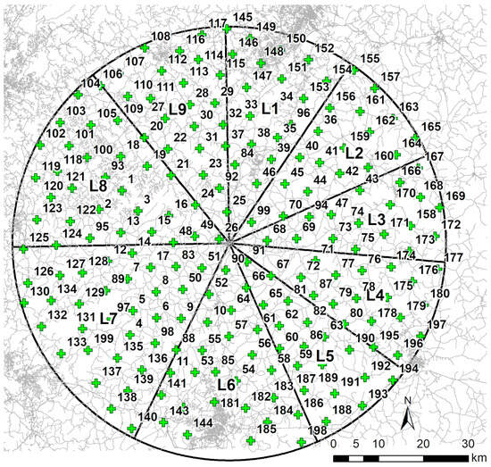
Figure 1.
Gretna database map (50-km radius) defining satellite storage locations (SSLs) for 150 k database. Subareas for nine load-outs shown, each with approximately the same total feedstock storage. Total of 199 SSLs (shown as crosses with the SSL number) in database. Figure first appeared in Resop et al. [9].
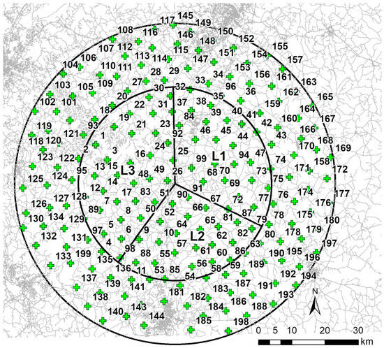
Figure 2.
Radius (29.1-km) on Gretna database map defining storage locations (SSLs) for 50 k database. Subareas for three load-outs shown, each with approximately the same total feedstock storage. Total of 71 SSLs (shown as crosses with the SSL number) in database.
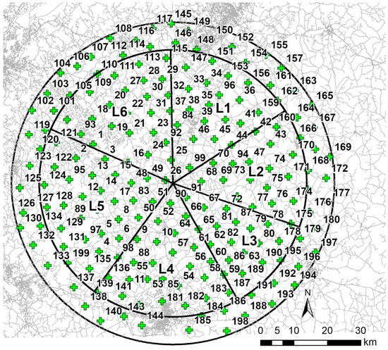
Figure 3.
Radius (40-km) on Gretna database map defining satellite storage locations (SSLs) for 100 k database. Subareas for six load-outs shown, each with approximately the same total feedstock storage. Total of 133 SSLs (shown as crosses with the SSL number) in database.
2.2. Definition of Load-Out Operations
For this study, hauling is conducted with a multi-bale handling system identified as the “rack system”. The rack is a 20-bale handling unit originally described by Grisso et al. [11]. Two racks, one each on two tandem trailers, gives a 40-bale truckload. The logistics plan calls for an empty tandem trailer set to be left at the SSL for loading while a loaded set is towed to the biorefinery, thus uncoupling the loading and hauling operations [12]. At the biorefinery, the loaded racks are lifted off and replaced with empty racks for return to any SSL where the load-out operation will have the next 40-bale load ready when the truck arrives.
The “ideal” load-out productivity defined for this study is 6 loads per 10 h day for each load-out operation. With uninterrupted operation, it is expected to take 1 h for an experienced operator to load 40 bales into the two racks [13]. Two pieces of equipment, a telehandler and a bale loader, are used. A bale loader, described by Grisso et al. [12], is moved into place and locked to the rear trailer. The operator then operates the telehandler to pick up bales individually, and load 10 bales into the bale loader, which pushes these bales into the bottom tier of the rear rack. The operator then moves the bale loader into position to load the front trailer, and proceeds to load 10 bales into the bottom tier of this rack. Then, the operator uses the telehandler to load the 20 bales into the top tier of the two racks, thus completing the full load of 40 bales.
The justification for 6 loads in an ideal 10 h haul day is as follows.
- The load-out crew will typically not start loading until the empty trailer set is unhooked, and the loaded trailer set is hauled away. This exchange time is the “load time” in the truck cycle time computation, and it is assigned to be 15 min for each load.
- The most impactful issue is the fact that the load-out operator will probably not always call the Feedstock Manager with a timely estimate of when they will have the load ready for pickup. Even if this is performed expeditiously, there is a low probability that the Feedstock Manager can dispatch a truck and have it arrive at the moment the last bale is loaded; there will always be delays.
Most commercial operations use a 70% estimate of ideal productivity as the achieved productivity in a commercial setting. The average achieved productivity used for the simulation performed here is then
Some days during a haul week, the productivity will be greater than 4.2 loads/d and some will be less. Over the 48 weeks of the hauling season, this analysis presumes that the average achieved productivity is 403.2 Mg/week for each week of operation across all load-outs. With 4.2 loads in a 10 h workday, the average “load-out cycle” is 2.38 h/load, as compared to 1 h/load to actually retrieve and load the 40 bales. Actual bale loading is, then, 42% of the workday. For some SSL layouts, time between loads might be used to stage bales so they can be retrieved and loaded faster when the truck arrives.
The time allowed in the simulation for moves between SSLs is 0.5 day for each move. The achieved productivity for a week where a single move occurs is
If two moves are required during a week (unloading of a small SSL is completed during the week and then there is a second move to the next SSL), then the achieved productivity for that week is
The analysis is performed for continuous operation of the load-outs. There are no holidays considered, no allowance for major equipment breakdowns (routine maintenance is already accounted for in the productivity estimate), and no delays due to weather (heavy rain, ice and snow on roads). These events are handled with “contingency days”, as discussed later. The 48-week hauling season for this study presumes that the biorefinery will shut down for maintenance and equipment upgrades for the final 3 weeks of August and will shut down 1 week at Christmas.
2.3. Definition of Load-Out Subareas
One load-out operation is assigned to each of the individual “pie-shaped” subareas shown in Figure 1, Figure 2 and Figure 3. Previous studies of load-out operations have shown that the average achieved load-out productivity, after considering the time to move between SSLs, will average about 60 Mg/d, as compared to the 67.2 Mg/d estimate for “continuous” operations. The following assumptions were used to estimate the number of load-outs required.
- Achieved average load-out productivity: 60 Mg/d
- Number of weeks for continuous operation: 45 (This gives 3 weeks × 6 d/week = 18 contingency days over a 48-week haul season, or about 0.4 days per week.)
Using these rules, the estimated number of subareas required for the 50 k database is 3 and the estimated number for the 100 k database is 6.
The estimated number of load-outs required for the 150,000 database is
An interesting question is now posed: do we design the logistics system for 9 load-outs or 10 load-outs? (Obviously, there can only be an integer number.) Suppose the achieved average productivity over 48 weeks (including contingency days) is 58 Mg/week, and we consider the total feedstock actually stored in the 199 SSLs (Gretna database). This computation says that 9.13 load-outs are required, and the decision is made to design for 9 load-outs.
2.4. Load-Out Sequencing within Subareas
The operation of the load-outs needs to be scheduled so that approximately the same number of truck operating hours are required to haul all loads loaded out each week. This provides the best opportunity to operate the truck fleet at maximum average productivity (Mg hauled per truck per week). For the 50 k database (Figure 2), the scheduling for load-out 1 (subarea L1) begins with SSLs closest to the plant (center of circle) and moves outward, a procedure identified as “in-to-out”. The load-out sequence chosen for load-out 2 is “out-to-in”, and that chosen for load-out 3 is “in-to-out”. The resulting load-out schedule is shown in Table 1; the numbers are the SSL numbers shown within the 29–1 km radius in Figure 2. Also given in Table 1 are the estimated days required to load-out each SSL. (Actual days will be higher than the estimate shown in Table 1 due to move time and contingency days.) The estimated load-out days ranged from 3 to 19.

Table 1.
Schedule of SSL load-out for 50 k database.
2.5. Procedure for Scheduling Movement between SSLs for each Load-Out Operation
Key constraint: no move between SSLs occurs until all full loads stored at a given SSL are shipped. Explanation of the load-out scheduling for the individual load-out operations is best performed with an example. This example uses SSLs 86, 60, and 56 from the load-out 2 schedule (shown in bold, Table 1) and begins with operations in week 7. At the beginning of this week, the load-out operation has completed the load-out of SSL 82 at the end on week 6 and has just moved to SSL 86. The operation loads out 369.6 Mg in week 7 because a move occurs during this week. The total stored in SSL 86 is 536.3 Mg, thus the operation loads out 166.7 Mg in week 8 to complete the load-out of SSL 86.
536.3 − 369.6 = 166.7 Mg
At SSL 60, the load-out operation loads out
to complete week 8 operations. It then loads out 403.2 Mg in week 9. (The amount loaded is 403.2, not 369.6, because the full week is available—no move occurs.) The amount stored in SSL 60 is 737.5, thus, the amount shipped from this SSL in week 10 is
369.6 − 166.7 = 202.9 Mg
737.5 (total stored) − 202.9 (shipped week 8) − 403.2 (shipped week 9) = 131.4 Mg
The operation then moves to SSL 56 where 811.5 Mg is stored. The amount shipped from SSL 56 to complete week 10 is
369.6 − 131.4 = 238.2 Mg
The amount shipped in week 11 is 403.2 Mg. The amount shipped in week 12 is
811.5 (total stored) − 238.2 (week 10) − 403.2 (week 11) = 170.1 Mg
The calculations proceed in this manner until all 22 SSLs in the load-out 2 schedule are shipped.
2.6. Number of Loads in Each SSL
The number of loads hauled from each SSL is calculated by dividing the total stored feedstock by the average load size, 16 Mg. This number is rounded down to eliminate partial loads. The operating plan calls for a “cleanup operation” to haul any remaining bales after the load-out operation has moved out. Cost of this cleanup operation, USD/Mg, is expected to be considerably higher; however, it is a necessary expense because any feedstock contract holder will want to sell all the biomass they produce and store.
2.7. Service Truck Scheduling
The load-out plan calls for a service truck to visit each active SSL load-out operation once each workday. The truck supplies fuel and routine maintenance needs, and the service technician provides assistance to the load-out worker, if needed. For this study, the service truck travel each day is calculated by summing the distance traveled when the service truck visits all load-outs in numerical order, for example, load-out 1, load-out 2, and load-out 3 for the 50 k database. In a mature industry, the route will be optimized, and the order the SSLs are visited will be chosen to minimize the total service truck travel each day.
To simplify the analysis, the service truck route for each week is defined for the SSLs being loaded out on Monday of that week. The travel on Monday is then multiplied by six to get the total travel estimate for a 6-d week. An example of service truck travel (km) is given below for week 7. Loadout 1 is loading out SSL 70, load-out 2 is loading out SSL 86, and load-out 3 is loading out SSL 49. The truck leaves from the biorefinery, visits all three load-outs, and returns to the biorefinery at the end of the day.
Travel to SSL 70 + from SSL 70 to SSL 86 + from SSL 86 to SSL 49 + return = total
17.1 + 59.5 + 72.1 + 9.7 = 158.4
17.1 + 59.5 + 72.1 + 9.7 = 158.4
Total travel for week 7 is then 6 × 158.4 = 950.4 km. If the average speed on rural roads is 70 km/h, the travel time is about 2.3 h/d, and if the technician spends a maximum of one hour at each of the three SSLs, the total time required is 5.3 h/d, or about half of the 10 h workday.
For the 100 k database, the six SSLs being loaded out on week 7 are 46, 171, 81, 183, 48, and 118, and the total travel is 384.1 km/d, or 2305 km/wk. Travel time is about 5.5 h/d, and, if the time at each SSL averages 1 h/d, then the total time required is 11.5 h/d. One service truck cannot complete the service in a 10 h workday and two service trucks will not be fully utilized. For this study, one service truck is specified, which means that each SSL being loaded out will average 45 min of service time, not 1 h.
For the 150 k database, the nine SSLs being loaded out on week 7 are 39, 165, 94, 197, 65, 64, 133, 15, and 110, and the total travel is 602 km/d, or 3612 km/wk. Travel time is about 8.6 h/d, and, if the time at each SSL averages 1 h/d, then the total time required is 17.6 h/d. Two service trucks operating 10 h/d can complete the required service, thus two are specified for this study.
2.8. Equipment Hauler Scheduling
An equipment hauler is dispatched from the biorefinery, travels to the SSL where load-out has been completed, moves the equipment to the next SSL in the load-out sequence, and then returns to the biorefinery. For example, the load-out sequence for load-out 1 in the 50 k database is SSLs 99, 68, 69, …, and 32 (Table 1). The equipment hauler hauls the equipment to SSL 99 to begin the haul season, and then returns to the biorefinery. When unloading of SSL 99 is complete, it travels to SSL 99, moves the equipment to SSL 68, and returns to the biorefinery. When SSL 68 unloading is complete, it travels to SSL 68 and moves the equipment to SSL 69 and returns to the biorefinery. This scheduling is complete until all moves are completed for the 48-week season. At the end of the haul season the equipment hauler travels to SSL 32 and hauls the equipment back to the biorefinery.
Total equipment hauler travel for the haul season is calculated by summing the total for all load-outs. This procedure is expected to give an upper bound for equipment hauler travel. Total hauls for load-out 1 (50 k database), including the initial and final hauls, is 20, and the totals for load-outs 2 and 3 are 23 and 31, respectively. If each haul takes 1 day, then the total use of the equipment hauler is 74 days, or about 26% of a 288-day haul season.
2.9. Definition of Truck Productivity
Truck ideal cycle time (Ti) is calculated using the following assumptions.
- Load time is defined as the total time to unhook a trailer set with empty racks and hook a trailer set with full racks at the SSL. For this study, the “load time” averages 15 min.
- Unload time is defined as the time to weigh in a truck at the receiving facility, sample for quality, lift off full racks from the trailer set and replace them with empty racks, and then weigh out. For this study, the “unload time” averages 20 min.
- Travel speed over rural roads averages 70 km/h.
For this study, a 1.4 multiplier is used to obtain truck achieved cycle time (Ta), thus
This increase is carried out in order to account for delays in loading (waiting at SSL) and unloading (waiting at receiving facility), plus delays due to traffic, particularly for travel through towns. The authors acknowledge that this is an ambitious achieved cycle time; however, it does provide a “baseline” estimate for the required truck fleet size.
3. Methodology for Cost Computation
3.1. Load-Out Cost
The plan presented here envisions that one worker will work four 10 h days, say Mon–Thu, then a second operator will work Fri–Sat and Mon–Tue of the next week, and this rotation will continue in order to provide a 60 h workweek over the 48-week season.
The same equipment operation at the SSL (telehandler and bale loader) used for the Resop et al. [9] study was used for this study. The telehandler is estimated to operate 1852 h/y of the total 10 h/d × 6 d/wk × 48 wk/y = 2880 h/y of load-out operation. This means the equipment operates, on average, 64.3% of each operating day. Telehandler cost (21.19 USD/h) and bale loader cost (10.34 USD/h) was calculated as shown in Resop et al. [9]. For this study, labor cost for the load-out worker is 25 USD/h with 25% benefits, thus the labor cost is 25 (1 + 0.25) = 31.25 USD/h. The load-out cost per operating day is then
where Ctheq = telehandler equipment cost (USD/h)
Cbleq = bale loader equipment cost (USD/h)
Llo = labor cost for load-out worker (USD/h)
Clo = total cost for load-out operations at SSL (USD/d)
3.2. Load-Out Worker Travel Reimbursement
It is expected that the load-out worker will provide their own transportation and report for work to the SSL being unloaded that day. (This is the procedure generally used for construction workers who report to a construction site to begin work.) Reimbursement for the worker’s transportation is calculated for a round trip each day to the SSL being unloaded that day (jth SSL). The distance is measured from the base (biorefinery at Gretna) to the SSL, thus it equals the haul distance. A column matrix is defined for the sequence of SSLs unloaded by each load-out. The number of rows in this matrix is n1, the number of SSLs unloaded. In the case of load-out 1, n1 = 19 (this column matrix, jlo1(i), is given in Table 1). For example, i = 1, j = 99 and i = n1, j = 32. The total annual travel payment (USD) for load-out 1 is
where ndayj = number of unload days for jth SSL (Table 1)
hdj = haul distance (km) for jth SSL
Tf = travel payment parameter = 0.364 USD/km.
In like manner, the total travel payment for the load-out 2 worker is
The total travel payment for the load-out 3 worker is
Dividing the total travel payment by the mass of all loads hauled by the individual load-out gives the load-out worker travel cost per Mg hauled.
3.3. Service Truck Cost
The ownership and operating cost (labor not included) for a service truck is 1.85 USD/km based on a typical cost for a truck servicing equipment on construction sites. This cost multiplied by the total annual travel gives the annual ownership and operating cost. The labor cost for this truck is
The number of technicians used for the computation was n = 0.5, 1, and 2 for the 50 k, 100 k, and 150 k databases, respectively.
3.4. Equipment Hauler Cost
The ownership plus operating cost (labor included) for the equipment hauler was estimated by Resop et al. [9] to be 3.10 USD/km, and this estimate is used here.
3.5. Computation of Truck Cost
The truck cost calculated for this study includes three main cost categories: truck tractor rental, driver (labor), and fuel. Recapping the business plan, the truck fleet is operated by the biorefinery, and its productivity is the responsibility of the Feedstock Manager. All maintenance for the truck tractors is covered by the rental contract. No cost is included for insurance, or for a fueling station at the biorefinery. Also, this comparison does not include the cost of the racks and rack trailers required for the rack system.
The current rental cost for a single-drive-axle, pintle-hitch truck tractor is 845 USD/week, thus the annual rental cost for a 48-week season is:
The labor cost for an operator, including benefits, is 31.25 USD/h. (A shift-work plan must be used to operate a 12 h haul day, 6 d/wk.) The annual labor cost for a 48-week season with six 12 h workdays each week is 108,000 USD per truck per year.
In this study, the only cost that varies with annual use is the fuel cost. Total fuel cost (based on 1.7 km/L consumption, at 1.31 USD/L) was calculated
where FC = fuel cost (USD/y)
Thd = total haul distance for annual operation of truck fleet (km/y)
3.6. Analysis
A separate GNU Octave [14] program was written to analyze each of the three databases. (These programs, with documentation, are available from the authors.) The output of each simulation was the achieved load-out productivity calculated for each load-out, each week of the 48-week season. Also, the total truck operating hours required to haul all loads each week (all load-outs as scheduled, no optimization) was calculated.
4. Results
4.1. Productivity of Load-Out Operations for all Three Databases
The calculated productivity for all load-outs in the 150 k database is given in Table 2. The entry in the “All” position is the average achieved productivity across all nine load-outs.
Table 2.
Load-out productivity for 150 k database.
A summary of the overall achieved productivity for all three databases is given in Table 3. As might be expected, the productivity is approximately the same across all three databases. Load-out operations are influenced by the average size of the SSLs, not by their location within the feedstock production region. Contingency ranged 0.4 to 0.6 days/load-out/week, which the authors judge to be a reasonable operating plan given the number of delays that might be expected for a short-haul operation over rural roads.
Table 3.
Summary of load-out productivity results.
The average SSL size in Table 2 was plotted to visualize the influence of this variable (Figure 4). The discontinuity at about 940 Mg average SSL size is caused by unexplained factors other than average SSL size in load-out subareas 1, 4, and 5.
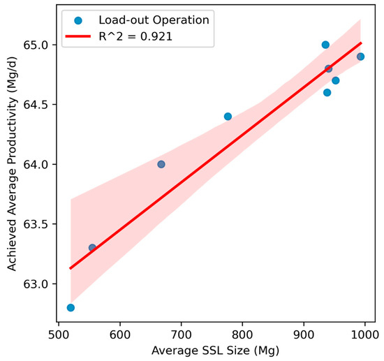
Figure 4.
Correlation between average SSL size and achieved average load-out productivity with continuous operation.
4.2. Hauling Results—50 k Database
The total loads shipped by the three load-outs were 3042, giving a total shipment of 48,672 Mg.
The total feedstock in storage in the SSLs, 19 (load-out 1) + 22 (load-out 2) + 30 (load-out 3) = 71 SSLs (total), was 49,865 Mg, thus the amount left for a clean-up crew was 2.4% of the total stored feedstock.
Total haul distance for all 3042 loads was 154,408 km, and the average haul distance for these loads was 25.4 km. The total truck operating time to haul all loads, using the 1.4 × ideal cycle time, was 5578 h. One truck hauling 12 h/d × 6 d/wk × 48 wk/y has 3456 h/y of available operating time. The minimum number of trucks required to haul all feedstock in a 48-wk season is
Is it practical for two trucks to haul all the feedstock? This means each truck will haul 3042/2 = 1521 loads/y = 31.6~32 loads/wk over a 48-week season. For a 6 d work week, each truck will average 5.3 load/d. To achieve this, the cycle time over a 12 h haul day must average 12/5.3 = 2.26 h/load.
The maximum ideal cycle time to haul from SSL 1 was 2.32 h. Average cycle time (ideal) across the 71 SSLs was 1.31 h. Using the 1.4 multiplier, if the achieved average cycle time is 1.31 × 1.4 = 1.83 h, thus, it is possible that a truck could achieve an average cycle time equal to the required 2.26 h; however, this is not realistic given the number of variables in a short-haul operation over rural roads.
The truck operating time required each week is given in Figure 5 for the 50 k database. Maximum truck productivity is achieved when the required truck operating hours is approximately the same each week. The varability shown in Figure 5 suggests that a better schedule for SSL unloading is needed.
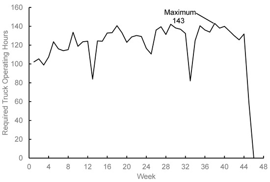
Figure 5.
Required truck operating hours each week for 50 k database.
This study provides no plan to optimize the hauling schedule for each week. If the Feedstock Manager knows, on Saturday of a given week, the harvesting schedule (from the feedstock contractors) and the hauling schedule, and thus knows where all full SSLs are located, then they can make adjustments to the load-out schedule for the upcoming week. This point will be re-emphsized in the conclusions.
Average required truck operating hours over the 48-week haul season is 5578/48 = 116.2~117 h/wk. With a two-truck fleet, the total available hauling hours is 144 h/wk. This means that the productivity factor over the 48-week season must average 117/144 = 0.81 for the truck fleet. This is quite optimistic—perhaps it could be achieved in a mature logistics system with a skilled crew.
Suppose a truck fleet of three trucks is specified. The available truck operating hours is now 216 h, and the productivity factor is 0.54. If three trucks haul 3042 loads in a 48-week haul season, the achieved average productivity must be
Truck productivity is then 21.1 loads/wk × 16 Mg/load = 338 Mg/wk/truck. The three load-outs loaded 3042 loads in a 48-week season, thus their average achieved productivity is 338 Mg/wk/load-out, the same as the truck fleet. Note, the load-out day is 10 h and the haul day is 12 h, thus the labor productivity of the load-out operator is greater than the truck driver productivity (Mg/h).
4.3. Summary of Hauling Results
The hauling parameters for the truck fleet are given in Table 4 for all three databases. The clean-up percentage ranges from 2.2 to 2.4%, which is judged to be an acceptable operating plan; hauling partial loads with the rack system is not a practical option.
Table 4.
Hauling parameters for three databases.
Required truck productivity is given in Table 5. The “productivity factor” is interpreted as follows. Using three trucks for the 50 k database means that 54% of the total operating hours must be productive hours for each truck. For the 100 k database, the productive hours for each of the six trucks must average 65% of the total available operating hours, and for the 150 k database the percentage is 74% for the nine-truck fleet.
Table 5.
Summary of truck productivity.
For three trucks to deliver the 50 k database loads over a 48-week season (12 h haul day, 6 d/week), the receiving facility must average a load every 200 min, which means the facility is not operating close to design capactity and per-Mg cost will be high. The six trucks delivering the loads for the 100 k database must average a load every 106 min, which is well within the 20 min average unload time used for the simulation. However, a receiving facility unloading the nine trucks delivering the loads for the 150 k database must average a load every 22 min, which is quite close to the 20 min unload time. These observations are made to highlight the importance of receiving facility design in the overall logistics system design.
The required truck operating hours for each week was plotted for the 100 k and 150 k databases. The variability was greater than that shown in Figure 5 for the 100 k database, but it was less for the 150 k database. Low variability in required truck operating each week is important because the most cost-effective operation is achieved when each truck operates approximately the same number of hours each week. A scenario where some of the trucks do not operate a full week should be avoided.
5. Discussion of Simulation Results
The load-out scheduling was performed using the assumption that each load-out would average 4.2 loads/d, giving a capacity of 25.2 loads for a full 6-d workweek. In actual practice, a load-out might ship 5, 4, 4, 3, 6, or 3 loads for days 1–6, respectively, for a total of 25 loads in that week. The next week, the load-out might ship 26 loads, thus the average for the two weeks is 25.5 loads/week. For the simulation results reported here, a load-out operation will average 4.2 loads/d × 6 day/week = 25.2 loads/week over an entire 48-week hauling season. The authors believe this average productivity can be achieved with a mature industry, but probably not during start-up.
The achieved average loads per day for the three load-outs in the 50 k database simulation was 3.8 loads/d (continuous load-out). The achieved loads/d is then 90.5% of the “ideal” 4.2 loads/d. This means that moves between SSLs reduces the productivity by 9.5%. Across the total season days, including the contingency days, the achieved loads/d is 3.5, or 83.3% of the 4.2 loads/d ideal.
The simulation results for the 100 k database show a reduction in productivity due to moves between SSLs of 7.1% and 16.7% when both moves and contingency days are included. The reduction in productivity for the 150 k database was 7.1% due to moves, and 14.3% when both contingency days and moves are included.
5.1. Load-Out Costs at SSLs
The load-out costs for the three databases are given in Table 6 as USD-per-Mg hauled over the 48-week season. Total worker travel increases as the production area increases, thus this payment increases. Small differences in load-out cost are due to the small differences in contingency days and the resulting modest differences in average achieved productivity. In this study, the total load-out cost is almost independent of the size of the feedstock production area.
Table 6.
Load-out cost for three databases.
5.2. Service Truck and Equipment Hauler Cost
The service truck and equipment hauler travel distances calculated for the three databases are given in Table 7, and the resulting costs are included in the total load-out cost (Table 8). There is about a 5.6% increase in total load-out operations cost as the feedstock production area triples in size. This increase is primarily due to the increase in travel cost for the worker, service truck, and equipment hauler. The operations cost at the SSL is not a function of location. The SSL can be located 5 km from the biorefinery, or 35 km, and the cost for loading bales into the racks will be approximately the same.
Table 7.
Total service truck and equipment hauler travel for the three databases.
Table 8.
Total cost for load-out operations for the three databases.
5.3. Truck Cost
Total truck cost (rental, operator, fuel) for the 50 k database is presented as an example. Cost for the rental and driver for the three trucks is
The fuel cost is
A cost per-Mg annual feedstock hauled (no clean-up included) is calculated
Cost of the two other databases is calculated using the same procedure and the results are summarized in Table 9. The truck cost increases only about 12% as the feedstock production area triples in size, which is less than might be expected given that average haul distance increased from 25.4 to 40.8 km, or 60%. Fuel cost increases about 63%, but this increase is somewhat “over shadowed” by the rental and labor costs.
Table 9.
Comparison of truck costs.
5.4. Comparison of Labor Cost for Load-Out and Truck Operations
The results for the 150 k database are used here. In considering this result, it is important to remember that the labor total for the nine load-out operations is 9 × 10 h/d = 90 h/d = 540 h/week, and the labor total for the nine-truck fleet is 9 × 12 h/d = 108 h/d = 648 h/week. If the labor cost is 31.25 USD/h (including benefits), then the labor cost for the load-out operation is
The labor cost for the truck operation is
The cost for hauling labor, on a per-Mg hauled basis, is about 20% higher than load-out labor. This suggests that the load-out operations should “wait for a truck” rather than a truck “wait at the SSL to be loaded”. It appears that the logistics system should be managed by the Feedstock Manager to minimize truck delays, and let the load-out operations wait, if that is required.
5.5. Future Considerations
Future simulations using the procedures developed for this study might include greenhouse gas (GHG) estimates and development of life cycle assessments (LCA) for certain bioproducts produced by the biorefinery. In addition, a stochastic analysis to determine the impact of a range of values for the key variables would add strength to the cost computations.
6. Conclusions
- When biorefinery capacity increases, and the feedstock production area triples in land area, the increase in truck cost (USD/Mg) is only about 12%. This is lower than might be expected, and it is explained by the selection of truck fleet size, and judicious scheduling of these trucks to maximize truck productivity (Mg/wk/truck) over the entire annual operation of the fleet. This result supports an industry design with central control of hauling.
- Approximately 0.5 contingency days per week is allowed for load-out operations over a 48-week season. Further study is needed to determine if this is a realistic logistics system design parameter.
- A key issue impacting load-out productivity is the wait time for a truck to arrive after a load is ready. This fact further reinforces the argument for central control of truck fleet scheduling to minimize this wait time.
- This study indicates (not proves) that it is more cost effective to have extra load-out capacity in order to minimize the average wait time for a truck to be loaded, rather than have an extra truck (larger fleet), and thus have a higher average wait time across all the trucks in the fleet. There is significant analysis technology for a logistics study to address this question. It is hoped this study will encourage a more robust study using these technologies.
- Variability in the required total truck operating hours each week shows an obvious need for optimization of SSL load-out scheduling to equalize required truck operating hours across the 48 weeks of fleet operation. The authors hope this study makes a strong enough case for central control of hauling that others will take on the challenge to apply the “tools and techniques” developed for analysis of other logistics systems to implement central control for their biorefinery location and surrounding feedstock production area.
Author Contributions
Conceptualization, J.S.C., R.D.G. and J.P.R.; methodology, J.S.C., R.D.G. and J.P.R.; software, J.S.C. and J.P.R.; validation, J.S.C., R.D.G., J.P.R. and J.I.; formal analysis, J.S.C.; investigation, J.S.C. and J.P.R.; resources, J.P.R. and J.I.; data curation, J.S.C. and J.P.R.; writing-original draft, J.S.C.; writing -review and editing, R.D.G., J.I. and J.P.R.; visualization, J.P.R.; supervision, J.S.C. project supervision, J.S.C. and J.I.; funding acquisition, none. All authors have read and agreed to the published version of the manuscript.
Funding
This research received no external funding.
Data Availability Statement
The datasets used for this study are available on request from J.S.C. jcundiff@vt.edu.
Conflicts of Interest
The authors declare no conflict of interest.
References
- National Academies of Sciences, Engineering, and Medicine. Safeguarding the Bioeconomy; The National Academies Press: Washington, DC, USA, 2020. [Google Scholar]
- Highfill, T.; Chambers, M. Developing a National Measure of the Economic Contributions of the Bioeconomy; U.S. Department of Commerce: Washington, DC, USA, 2023.
- Daystar, J.; Handfield, R.; Golden, J.S.; McConnell, E.; Pascual-Gonzalez, J. An Economic Impact Analysis of the US Biobased Products Industry. Ind. Biotechnol. 2021, 17, 259–270. [Google Scholar] [CrossRef]
- Golden, J.S.; Handfield, R.; Pascual-Gonzalez, J.; Agsten, B.; Brennan, T.; Khan, L.; True, E. Indicators of the US Biobased Economy; USDA: Washington, DC, USA, 2018.
- CFR. 7 § 3201 Guidelines for Designating Biobased Products for Federal Procurement; Code of Federal Regulations; CFR: Washington, DC, USA, 2005. [Google Scholar]
- 6866-11; Standard Test Methods for Determining the Biobased Content of Solid, Liquid, and Gaseous Samples Using Radiocarbon Analysis. ASTM International: West Conshohocken, PA, USA, 2011.
- USDA BioPreferred Product Categories. Available online: https://www.biopreferred.gov/BioPreferred/faces/pages/ProductCategories.xhtml (accessed on 27 June 2023).
- Lynd, L.R.; Wyman, C.; Laser, M.; Johnson, D.; Landucci, R. Strategic Biorefinery Analysis: Analysis of Biorefineries; National Renewable Energy Lab: Golden, CO, USA, 2005. [Google Scholar]
- Resop, J.P.; Cundiff, J.S.; Grisso, R.D. Central Control for Optimized Herbaceous Feedstock Delivery to a Biorefinery from Satellite Storage Locations. AgriEngineering 2022, 4, 544–565. [Google Scholar] [CrossRef]
- Resop, J.P.; Cundiff, J.S.; Heatwole, C.D. Spatial analysis to site satellite storage locations for herbaceous biomass in the piedmont of the Southeast. Appl. Eng. Agric. 2011, 27, 25–32. [Google Scholar] [CrossRef]
- Grisso, R.D.; Cundiff, J.S.; Comer, K. Multi-bale handling unit for efficient logistics. AgriEngineering 2020, 2, 336–349. [Google Scholar] [CrossRef]
- Grisso, R.D.; Cundiff, J.S.; Sarin, S.C. Rapid truck loading for efficient feedstock logistics. AgriEngineering 2021, 3, 158–167. [Google Scholar] [CrossRef]
- Hess, J.R.; Kenney, K.L.; Ovard, L.; Searcy, E.M.; Wright, C.T. Uniform-Format Solid Feedstock Supply System: A Commodity-Scale Design to Produce an Infrastructure-Compatible Bulk Solid from Lignocellulosic Biomass; Idaho National Lab: Idaho Falls, ID, USA, 2009. [Google Scholar]
- Eaton, J.W.; Bateman, D.; Hauberg, S.; Wehbring, R. GNU Octave Version 8.2.0 Manual: A High-Level Interactive Language for Numerical Computations; (No Location). 2023. Available online: https://www.academia.edu/15210344/GNU_Octave_A_high_level_interactive_language_for_numerical_computations (accessed on 12 July 2023).
Disclaimer/Publisher’s Note: The statements, opinions and data contained in all publications are solely those of the individual author(s) and contributor(s) and not of MDPI and/or the editor(s). MDPI and/or the editor(s) disclaim responsibility for any injury to people or property resulting from any ideas, methods, instructions or products referred to in the content. |
© 2023 by the authors. Licensee MDPI, Basel, Switzerland. This article is an open access article distributed under the terms and conditions of the Creative Commons Attribution (CC BY) license (https://creativecommons.org/licenses/by/4.0/).