1. Introduction
Agricultural territories, especially fertile expanses of arable land, stand recognized as invaluable assets pivotal to food production, necessitating meticulous stewardship [
1]. The emphasis on the precise delineation of these lands is underscored by their significant bearing on numerous operational facets. For instance, meticulous mapping is indispensable for orchestrating effective land use planning and management, fostering an environment in which lands are exclusively earmarked for agricultural undertakings, thereby averting soil degradation and environmental detriment [
2].
By crafting clear agricultural boundaries, planners can orchestrate optimized land usage, safeguarding vital resources from non-agricultural encroachment. This approach is fundamental to sustaining the health and productivity of farmlands, enabling farmers and land managers to exert finer control over natural resources such as water and soil. Recognizing the exact contours of croplands, for instance, facilitates the targeted application of irrigation, averting water wastage and thereby conserving precious water resources [
3].
Moreover, this precision plays a vital role in soil management, a critical element in sustaining soil fertility and optimizing crop yields [
4]. The legal ramifications are equally significant, with the clear delineation of property and tenure rights being central to fostering sustainable land utilization. A clear demarcation prevents disputes and encroachment, averting potential conflicts and legal complications, thus fostering a conducive environment for the effective conservation and management of agricultural lands.
Furthermore, it is noteworthy that adept agricultural management often hinges on the precise knowledge of the land’s extent and crop types cultivated therein. This knowledge empowers policymakers to devise comprehensive strategies addressing critical concerns, such as food security, land utilization, and environmental safeguarding. For instance, well-defined land boundaries can catalyze the formulation of policies that bolster food crop production while thwarting the conversion of agricultural lands for non-agricultural purposes [
5].
Monitoring agricultural efficacy demands the procurement of precise and dependable data pertaining to the extent of agricultural lands [
6,
7,
8,
9]. The exact demarcation of these lands facilitates data acquisition, which can critically influence the assessment of agricultural performance metrics, such as yield, soil quality, and environmental impacts. This data repository becomes a cornerstone in guiding resource distribution decisions and shaping agricultural policies.
Accurate field boundary acquisition can be achieved through various techniques, including traditional survey methods and contemporary remote sensing technologies. Established methods, such as total station surveying [
10], GPS/GNSS surveying, and unmanned aerial photography [
11,
12], offer reliable, albeit sometimes time-consuming, solutions for acquiring precise field boundaries. While tachymetric surveying promises high accuracy, it demands a considerable time investment and specialized personnel. Conversely, GPS surveying offers a more economical and swifter alternative, despite being potentially prone to environmental disruptions.
Aerial photography has emerged as a proficient tool, capable of capturing extensive agricultural expanses with commendable accuracy. Additionally, remote sensing avenues such as satellite imagery and LiDAR [
13] employ aerial or satellite photography to secure precise field boundaries. While satellite imagery offers extensive coverage capabilities, its efficacy is somewhat contingent on the resolution of the images captured. LiDAR, on the other hand, guarantees high precision, albeit at a higher cost and requiring skilled personnel for its operation.
The methodology chosen for detecting field boundaries is contingent upon a myriad of factors, including the scale of the field, the resources at one’s disposal, and the requisite degree of accuracy. Although survey techniques promise precision, they are often marred by their time-intensive nature. Conversely, remote sensing methodologies, though efficient and capable of encompassing vast agricultural areas, are not devoid of challenges. A critical aspect of these methods is the role of operators in delineating land boundaries, a task that necessitates specialized skills and software applications, predominantly geographic information systems. These methodologies, though exact, often entail diminished productivity, with a notable issue being the subjectivity inherent to interpreting the features demarcating agricultural land boundaries. Thus, enhancing the objectivity and bolstering the productivity of these interpretations, without sacrificing the quality of boundary recognition, emerge as paramount objectives for the advancement of remote sensing methodologies. In light of these challenges, we propose the integration of convolutional neural networks (CNNs) as a progressive solution.
In recent years, CNNs have experienced a surge in popularity in the domain of object boundary mapping. Their ascent can be attributed to their ability to discern and delineate object boundaries within images with acute accuracy, thereby positing them as ideal candidates for initiatives such as agricultural boundary delineation [
14,
15,
16,
17].
A significant advantage of utilizing CNNs for object boundary mapping is their intrinsic ability to assimilate and adapt to the distinctive features and nuances of the objects under scrutiny. Through the training phase on an image dataset characterized by known object boundaries, the network acquires the capability to discern the patterns and attributes unique to those objects. This, in turn, facilitates the accurate mapping of boundaries for analogous objects in subsequent images [
18]. Additionally, CNNs are proficient at managing images of high complexity and variability. In the context of agricultural mapping, imagery often encapsulates diverse elements such as crops, soil variants, and water bodies, which present considerable challenges in terms of accurate differentiation and mapping. Nevertheless, CNNs demonstrate the capacity to analyze these multifaceted images and identify object boundaries with remarkable precision, despite their inherent complexity and variability [
19].
Furthermore, CNNs are adept at delineating object boundaries with a high degree of accuracy and efficiency, establishing them as potent instruments for mapping extensive land parcels. This attribute is particularly salient in the sphere of agricultural land mapping, wherein the rapid and accurate mapping of large swathes of land is pivotal to fostering effective land use planning and management strategies.
Embarking on this study, our primary objective was to conceptualize an automated mechanism for detecting the boundaries of agricultural lands, leveraging the capabilities of deep neural networks alongside Sentinel 2 multispectral imagery. To attain this objective, the following tasks were outlined and completed:
Acquire and preprocess Sentinel 2 imagery for use in training and testing deep neural networks.
Select an appropriate deep neural network architecture for the boundary detection task.
Train and validate a deep neural network using labeled crop boundaries on Sentinel 2 imagery.
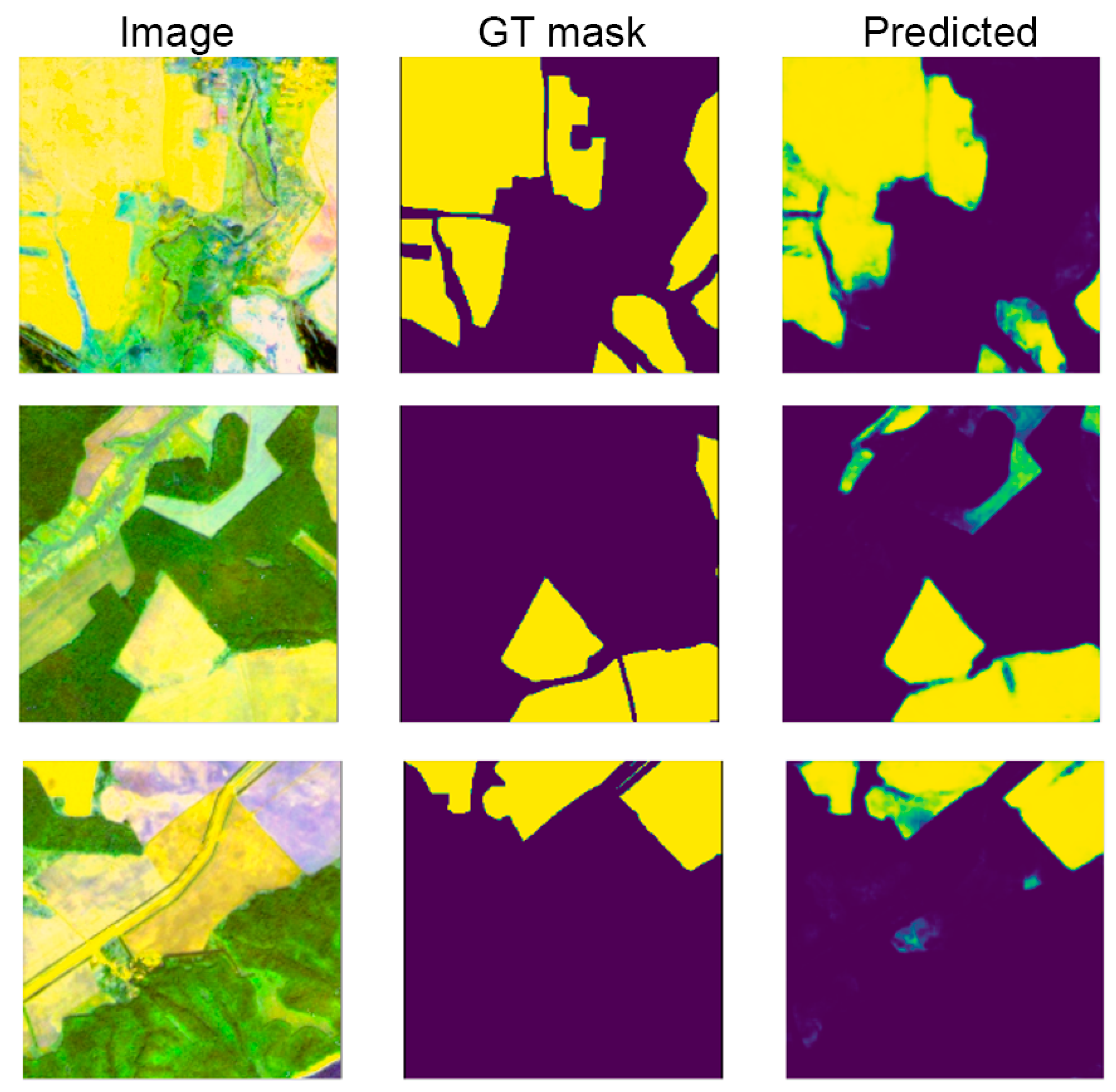
Evaluate the performance of the trained network on validation images by comparing the predicted boundaries to the ground truth data.
Analyze the results of the experiment and conclude the effectiveness of using deep neural networks and multispectral Sentinel 2 imagery for automatic cropland boundary detection.
2. Materials and Methods
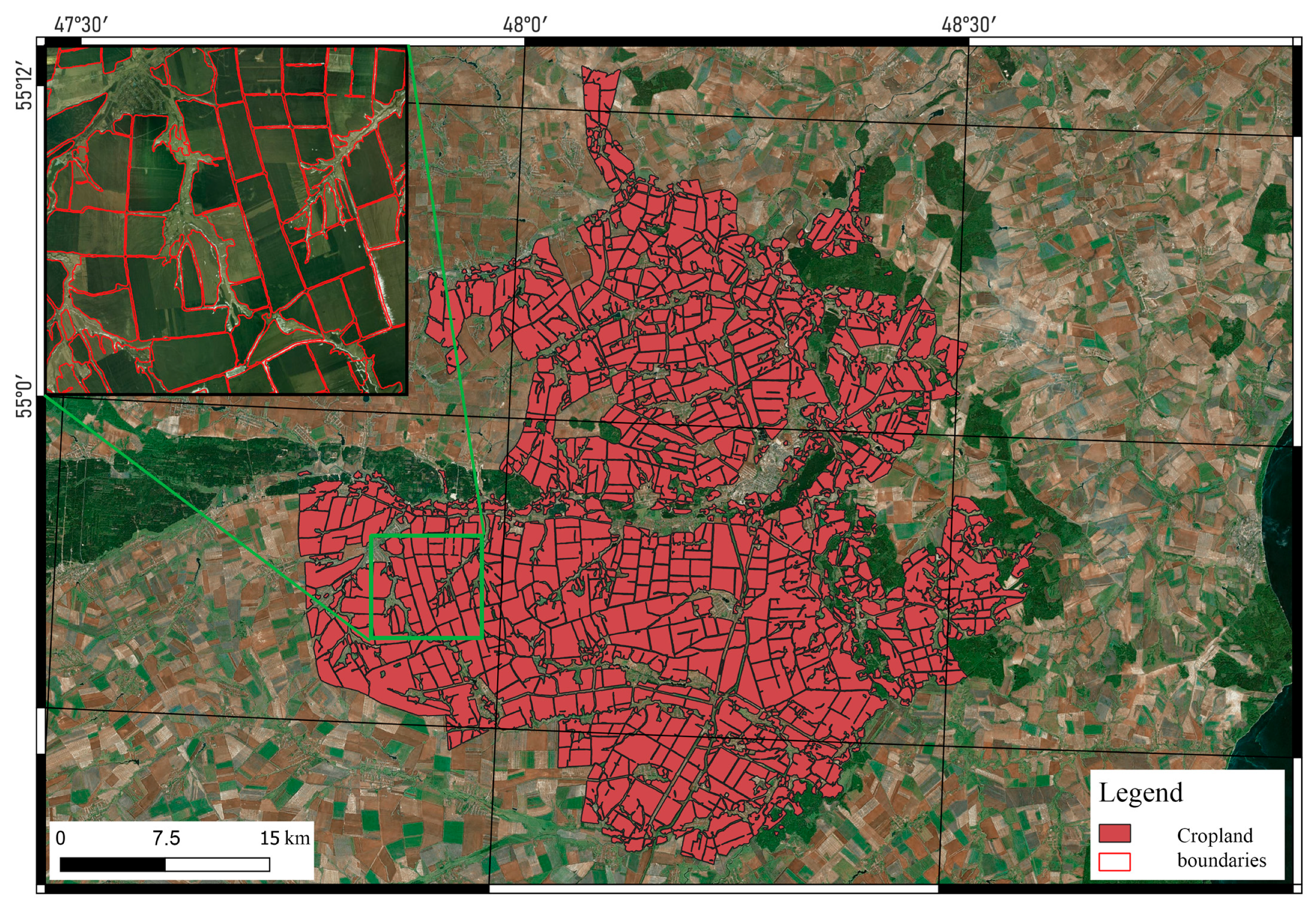
Buinsky municipal district was chosen as the study area. Buinsky district is a district of the Republic of Tatarstan, which is a federal subject of Russia. The district is located in the western part of Tatarstan and covers an area of about 1500 square kilometers. It borders the Apastovsky district to the north, the Tetyushsky district to the east, the Drozhzhanovsky district to the south, and the Yalchiksky district of the Chuvash Republic to the west [
20].
The landscape of Buinsky district is characterized by hills and forests, with many rivers and streams flowing through the area. The largest river in the district is the Sviyaga River, which flows through the entire district from north to south. Other important rivers are Cherka and Karla.
The climate of the Buinsky district is moderately continental, with cold winters and warm summers. The average temperature in January, the coldest month, is about −11 degrees Celsius, and the average temperature in July, the warmest month, is about 19 degrees Celsius. The area receives an average of 500–600 mm of precipitation per year, with most of it falling in the summer months.
The population of Buinsky district is about 44,000 people, with most of the population living in rural areas. The largest settlement area is the town of Buinsk, which is located in the central part of the district and serves as its administrative center.
The economy of the Buinsky district is mainly based on agriculture, with crops such as wheat, barley, and potatoes. Animal husbandry is also an important industry in the district, and cattle, pigs, and poultry are raised. In addition to agriculture, the district also has several small businesses, including manufacturing and retail trade.
The choice of the area was determined by its agricultural focus and the importance of being able to correctly and accurately determine the boundaries of its arable land.
To solve the problem of semantic segmentation, i.e., delineation of agricultural land boundaries, the Linknet architecture was used, which is a deep neural network architecture widely used for image segmentation tasks [
18]. It is based on a fully convolutional network (FCN) and has an encoder–decoder structure with skips between the encoder and decoder. The skip links help preserve spatial information during the oversampling process and allow the decoder to learn from the high-resolution characteristics of the encoder. This makes Linknet well suited for tasks such as object detection and segmentation [
21].
Linknet consists of several layers of convolution and merging operations in the encoder, followed by a corresponding number of layers of transpose convolution and upsampling operations in the decoder. Pass-through links are added between the corresponding layers in the encoder and decoder. To speed up convergence during training, Linknet also uses batch normalization and corrected linear units (ReLU).
To further improve Linknet’s performance, transfer learning using pre-trained models has been applied. A commonly used pre-trained model is DenseNet [
22], which is a deep neural network architecture that uses dense connections between layers to improve information flow and gradient propagation.
To use DenseNet for transfer learning, the pre-trained model is first tuned on a large dataset such as ImageNet to learn common features such as edges, corners, and textures. The weights of the pre-trained model are then fixed, and the Linknet decoder network is attached to the last few layers of the DenseNet model. The entire network is then trained on the target dataset to learn specific features to solve the segmentation problem.
Another popular pre-trained model for transfer learning that has been used is EfficientNet [
23], which is a family of deep neural network architectures that scale in size and complexity to improve performance on a variety of tasks. EfficientNetB3 is one of the most commonly used versions and has shown superior performance compared to that of other pre-trained models, such as ResNet and Inception.
To use EfficientNetB3 for transfer learning, the same approach can be used as with DenseNet. The pre-trained model is trained on a large dataset such as ImageNet, and then the Linknet decoder network is attached to the last few layers of the EfficientNetB3 model. The entire network is then trained on the target dataset to learn specific features for the segmentation task.
In the preliminary phase of our research, we embarked on a comprehensive scrutiny of credible data repositories, encompassing high-resolution satellite imagery, up-to-date land use maps, and widespread field investigations. This multifaceted analysis paved the way for the discernment and categorization of diverse land cover segments prevalent within the focal area of our study.
The successful categorization of these segments stemmed from an in-depth acquaintance with the regional agricultural landscape, a knowledge base that was significantly augmented through meticulous field surveys. These surveys stood as an invaluable resource, channeling firsthand observations and expert insights, thereby facilitating the precise demarcation of various land cover classifications.
To fortify the reliability and accuracy of these user-generated class values, we instituted a process of cross-verification. This approach involved aligning the identified class values with scholarly sources and established databases, thereby enhancing their legitimacy and relevance within the context of the study region.
Upon the affirmation of these class values, they were integrated as benchmarks in the validation phase, serving as a trusted reference point for scrutinizing the predictive prowess of the model. This approach fostered a detailed assessment of the model’s output, spotlighting its strengths and pinpointing potential avenues for refinement.
This strategy not only allowed for nuanced insight into the model’s efficacy but also charted a pathway for prospective advancements, aimed at perpetually honing its accuracy in delineating cropland boundaries. Through a methodical and objective selection and justification of user-defined class values, we have underscored their pivotal role in the validation paradigm. Consequently, this has elevated the trustworthiness and precision of the model’s predictions in mapping cropland boundaries, paving the way for a promising progression of continual improvement and refinement in the subsequent stages of this research endeavor.
The training, verification, and implementation of the model were performed using Sentinel 2 satellite imagery [
24]. Sentinel 2 imagery is widely recognized as one of the best data sources for agricultural field delineation. Using Sentinel 2 imagery for this purpose has several advantages.
First, Sentinel 2 imagery provides high-resolution data with a spatial resolution of up to 10 m, which is suitable for detecting small-scale objects such as agricultural field boundaries. These high-resolution data allow you to accurately define and delineate field boundaries, making it easier to map and manage agricultural land.
Second, Sentinel 2 imagery provides data in 13 spectral bands, including visible, near-infrared, and shortwave infrared. Different types of land cover, including vegetation, soil, and water bodies, can be identified using this spectral information. This is particularly important for agricultural mapping. It is necessary to distinguish between crops, bare soil, and other features, such as irrigation systems and water bodies.
Third, Sentinel 2 imagery has a high temporal resolution: images are acquired every 5 days. This frequent data collection allows farmland to be monitored throughout the growing season, providing information on crop growth, health, and productivity. This information is critical for effective land use planning and management, allowing farmers and land managers to make informed decisions about crop management, irrigation, and fertilization.
Another benefit of Sentinel 2 imagery is its free availability through the European Space Agency’s Copernicus program. This makes it an affordable and accessible option for mapping agricultural field boundaries, especially for small farmers and land managers who do not have access to expensive commercial imagery.
Finally, Sentinel 2 imagery is supported by a range of image processing and analysis software and tools. These include open-source tools, such as QGIS and the Sentinel Application Platform (SNAP), which provide various functions for processing and analyzing Sentinel 2 imagery for agricultural land mapping.
The analysis used a three-channel composite Sentinel 2 image for the 2021 growing season, with the Normalized Difference Vegetation Index (NDVI) standard deviation as channel 1, the infrared spectral band (833–835.1 nm) as channel 2, and the red channel (664.5–665 nm) as channel 3. This combination makes it possible to better distinguish the ground line, which theoretically should correspond to unpaved roads separating cropland, as well as cut-off forest areas and pastures, which have less variability in the vegetation curve than plowed land.
Our methodology hinges on utilizing the robust capabilities of Google Earth Engine (GEE) [
25], a cloud-based platform for planetary-scale geospatial analysis. Python libraries such as earthengine-api, the Python client for GEE, eemont [
26], an extension of earthengine-api for advanced preprocessing, and geemap [
27,
28], an interactive mapping tool, are utilized.
For our study, we prepare data from the Sentinel 2 surface reflectance (COPERNICUS/S2_SR) [
29] dataset that intersects our region of interest. Images captured between April and July 2021 are preprocessed (non-vegetation period), and the Normalized Difference Vegetation Index (NDVI), a crucial indicator of vegetation health, is calculated for each.
The standard deviation of the NDVI is computed across the image collection, providing insights into the temporal variability of vegetation health. Median reflectance values are also calculated for the near-infrared (B8) and red (B4) bands of the Sentinel 2 dataset. These images are multiplied by a factor of 10,000 to convert them from floating-point numbers to short integers, optimizing storage space.
The processed layers are combined into a single composite image, and this composite is then added to the interactive map, providing a visual representation of the calculated indices (source code available in Google Colab via
https://clck.ru/35Zmrj, accessed on 1 January 2023).
Finally, we initiate an export task that sends the composite image to Google Drive in the form of a GeoTIFF file. The image is exported at a scale of 10 m using the EPSG:32639 coordinate reference system, ensuring spatial consistency with other geospatial datasets.
The resulting composite is converted to uint8 format with a 5% percentile cutoff to minimize the effect of noise and to maintain an 8-bit color scale in each channel, which is required for pattern recognition using convolutional neural networks.
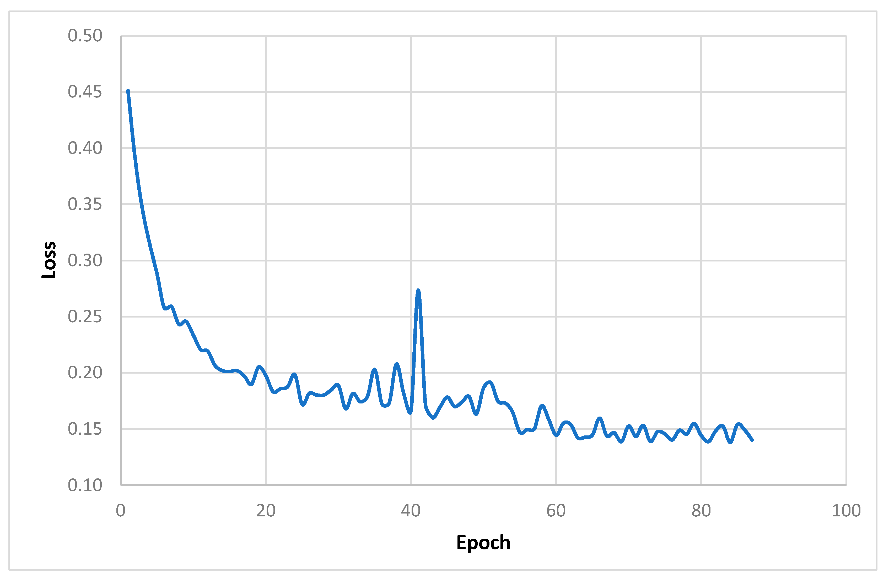
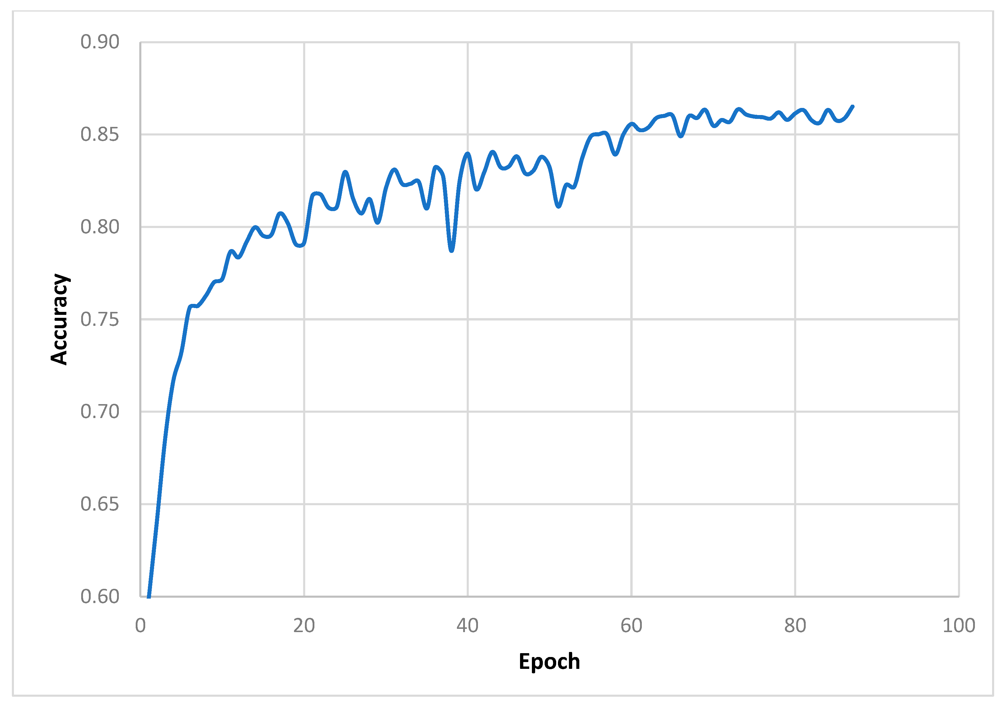
From the obtained image, an area of ~45,000 ha is selected for training and testing the neural network. For this purpose, continuous manual extraction of all cultivated areas is performed using WorldView-3 imagery with 0.5 m resolution, and the resulting vector layer is rasterized using a satellite image raster grid with 10 m resolution. The resulting image–mask pair is sliced by a floating window into 256 × 256 pixel squares called patches, with 50% of the previous patch’s neighbor captured. The process begins with parameter initialization, which defines key inputs such as input files, labeled files, window size, stride, label type, and output format. This initialization phase allows for flexibility and customization to meet different geospatial needs. Once the parameters are set, the methodology proceeds with data verification to ensure the consistency and integrity of the input files. This step validates that the input files are single-band rasters with matching attributes such as rows, columns, projections, and transformations. By verifying the input data, subsequent analysis can rely on reliable and consistent geospatial information. After data verification, the methodology focuses on feature and label generation. Input files are processed to construct feature and label arrays, in which labels are classified based on user-defined class values. This step enables the extraction of relevant information from the geospatial data and prepares it for subsequent machine learning tasks. In addition, a coordinate mesh is created to accurately position the geospatial data. This mesh consists of top-left coordinates that ensure proper alignment and geospatial reference throughout the generated image patches. These image patches, or “chips”, are then generated based on the specified step and window size, allowing for efficient data organization and analysis. This results in a dataset in which 80% of the data are used to train the neural network and 20% are used for validation and testing. The training is performed in Python 3.8 environments using the TensorFlow machine learning framework. To artificially increase the volume of the training sample, the filters compression-stretching, mirroring, cropping with rotation, etc., are applied to the images, which allows us to increase the volume of the training sample up to more than 30,000 pairs of the image mask. To minimize the risk of overfitting and underfitting, iterative learning monitoring functions are used, which reduces the learning rate when it reaches a “learning plateau”, but stops learning if the loss function does not decrease over 5 learning epochs. The Jaccard coefficient, a measure of the consistency of the predicted image with the true image, is used as the loss function.
The trained neural network model is applied to the satellite image of the entire Buinsky district.


