Novel Route Planning System for Machinery Selection. Case: Slurry Application


Abstract
1. Introduction
- Decompose the fertilizing operation, by considering the operations elements (such as performing the main task) and unproductive elements (such as turnings in the headland part and idle transportation), to determine the operational performance of the machinery. Farmers’ current practices are used for validating and benchmarking the proposed algorithm and model.
- Develop an algorithm and tool to solve this specific field coverage problem with optimized application rates and minimized driving distances for all individual tracks in the field.
- Develop an approach and tool to help farm managers to select the proper tank volume for the machinery system given specific constraints.
2. Materials and Methods
2.1. Characteristics of the Slurry Application
2.2. Mathematical Formulation
2.3. Solution Representation
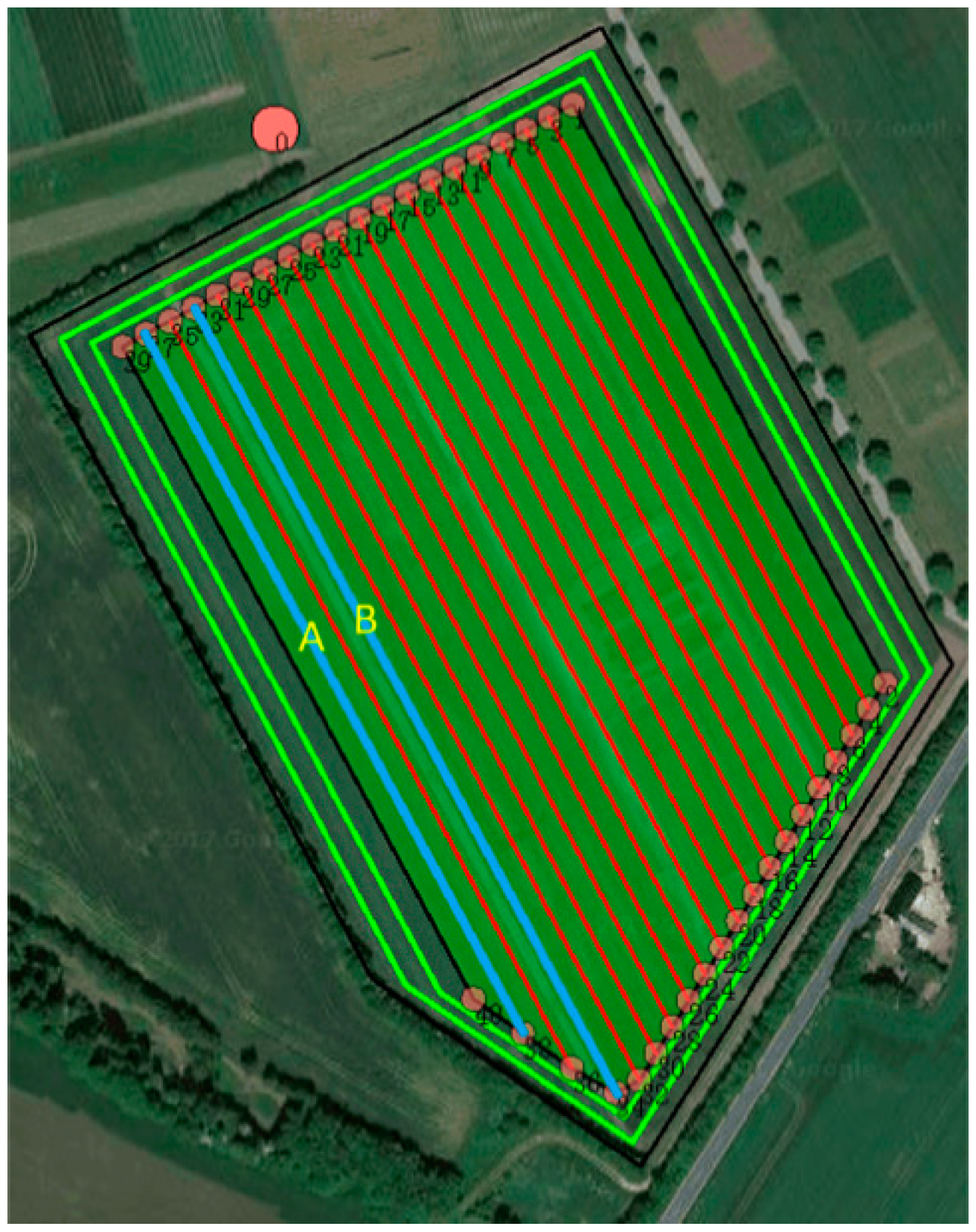
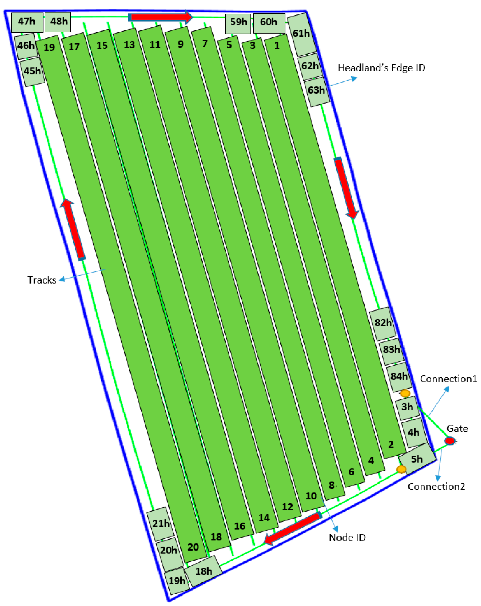
2.3.1. Field Representation
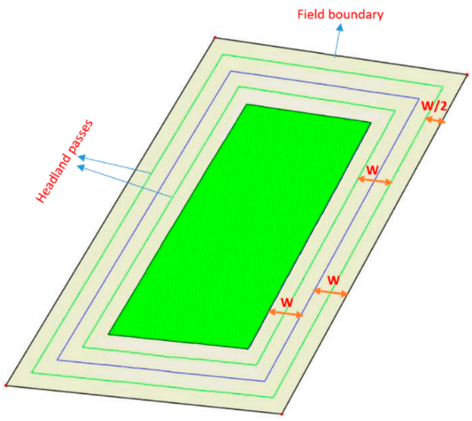
Headland Area Generation
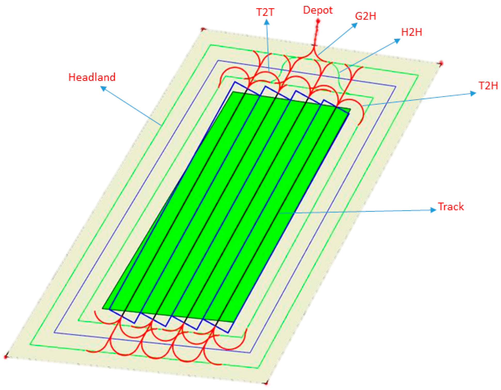
Track Generation and Edge Type
- Gate to Headland (G2H): two edges connect the gate to the headland path
- Headland: the connection between two subsequent vertices in headland path
- Track: the connection between two pairs of nodes (two ends of a fieldwork area). Once a vehicle selects one end as the track entry, it has to finish the operation in the current track and exits at the opposite end of the current track before moving to another track.
- Track to Headland (T2H): the connection between track nodes and vertices in the headland path
- Track to track (T2T): the connection between the end nodes of two adjacent tracks
- Headland to headland (H2H): the connection between two headland paths
2.4. Optimization Algorithm
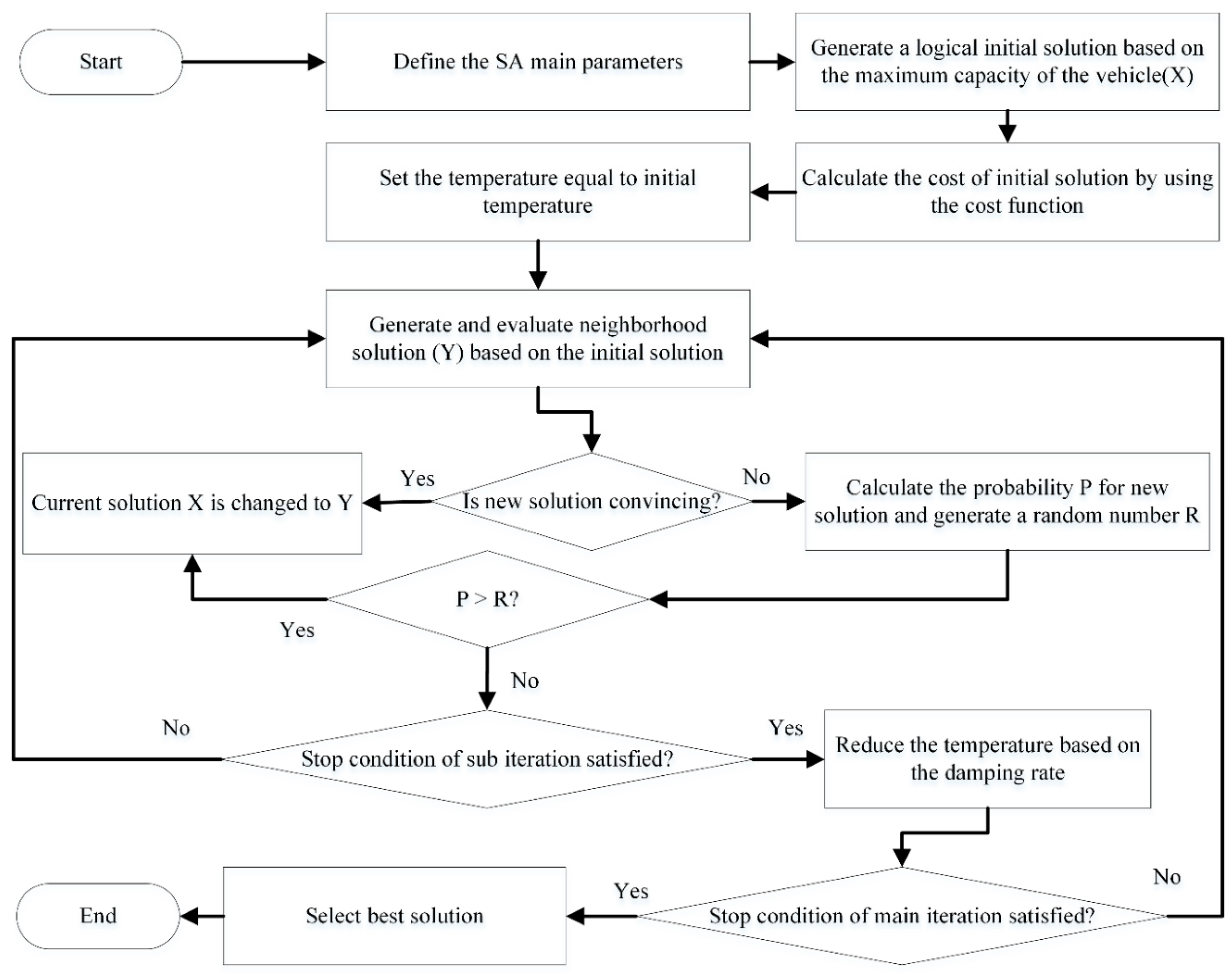
2.4.1. SA Algorithm
Neighborhood Operators
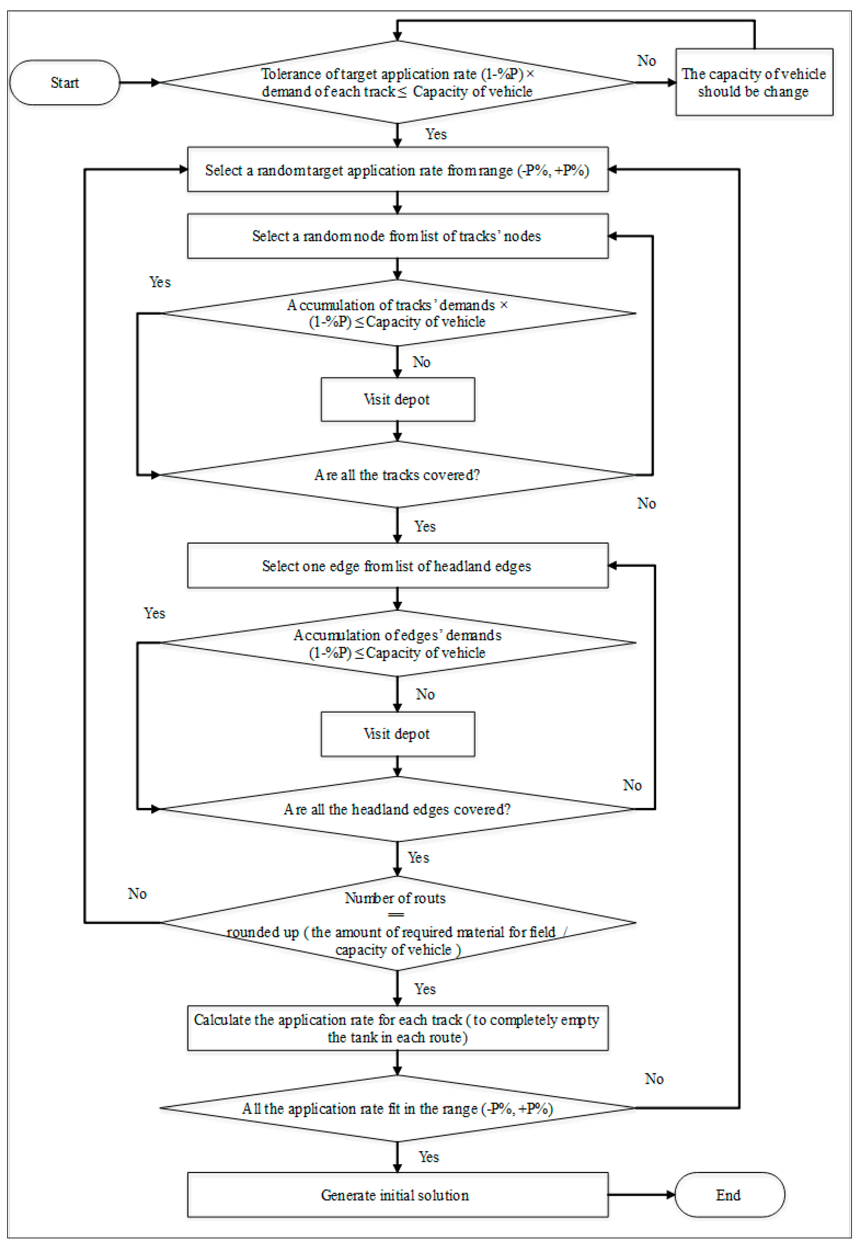
Initial Solution
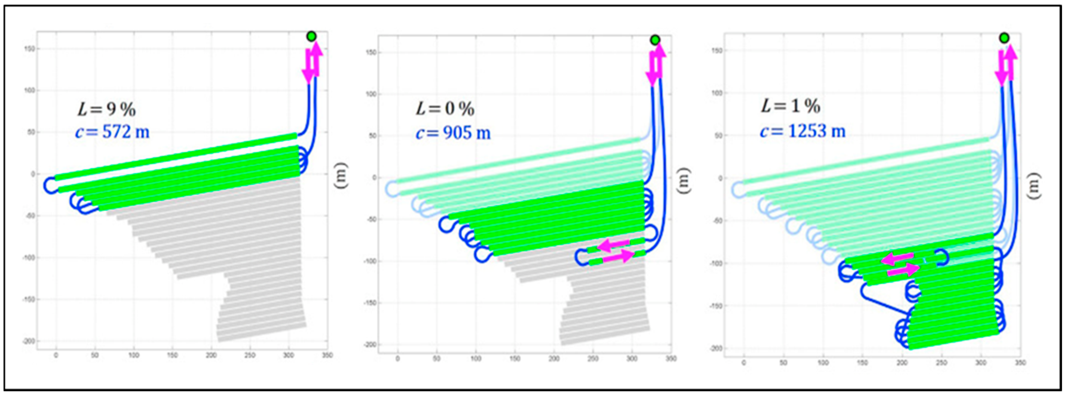
2.4.2. Application Rates
2.4.3. Cost Matrix Generation
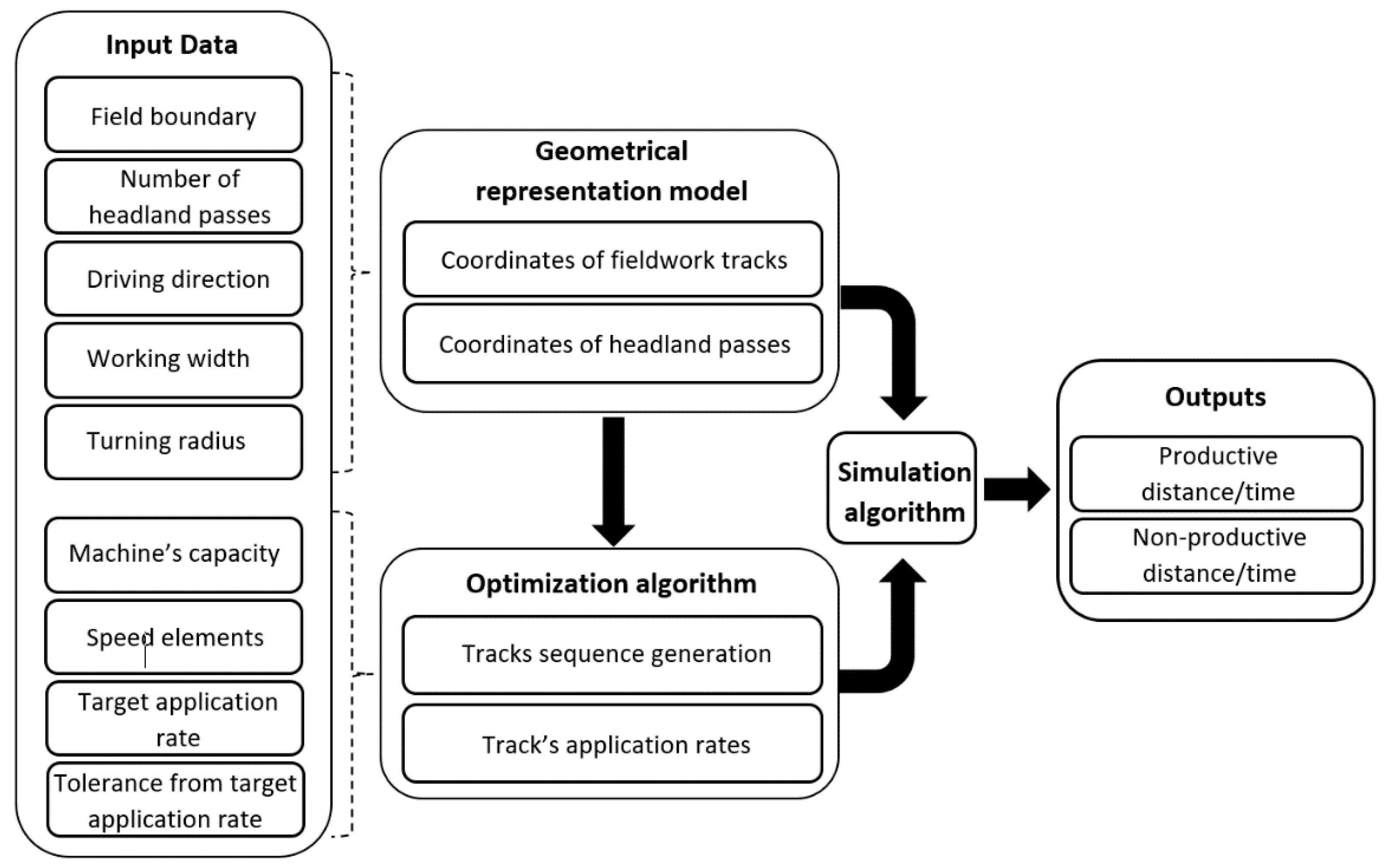
2.5. Simulation Algorithm
3. Results
The Strategic Decision for Machinery Selection
4. Discussion
5. Conclusions
Author Contributions
Funding
Conflicts of Interest
Appendix A

| Node/Edge ID | Application Rate (L/m2) | Node/Edge ID | Application Rate (L/m2) |
|---|---|---|---|
| 1 | 3.114799011967676 | 48 h | 3.114774926773009 |
| 4 | 3.1147990119676754 | 47 h | 3.114774926773009 |
| 5 | 4.6061000129481195 | 46 h | 3.1147806166643486 |
| 8 | 4.6061000129481195 | 45 h | 3.1147736783248767 |
| 9 | 4.60610001294812 | 44 h | 3.114774926773009 |
| 12 | 4.36275440399874 | 43 h | 3.114774926773009 |
| 13 | 4.36275440399874 | 42 h | 3.1147762950571463 |
| 16 | 4.36275440399874 | 41 h | 3.114800113322044 |
| 17 | 4.36275440399874 | 40 h | 3.114774926773009 |
| 20 | 4.60610001294812 | 39 h | 3.114774926773009 |
| 84 h | 3.114833305549154 | 38 h | 3.1147938549403227 |
| 83 h | 3.114774926773009 | 37 h | 3.1148003337060293 |
| 82 h | 3.114774926773009 | 36 h | 3.114774926773009 |
| 81 h | 3.1148054910798435 | 35 h | 3.114774926773009 |
| 80 h | 3.114782546605226 | 34 h | 3.1147341965638637 |
| 79 h | 3.114793927303264 | 33 h | 3.1148008560895373 |
| 78 h | 3.114801606808676 | 32 h | 3.114774926773009 |
| 77 h | 3.114779348093042 | 31 h | 3.114821230419206 |
| 76 h | 3.1148156792952406 | 30 h | 3.114896876687335 |
| 75 h | 3.1147597405964764 | 29 h | 3.1148156792952406 |
| 74 h | 3.1147849713320523 | 28 h | 3.114802898522297 |
| 73 h | 3.114774926773009 | 27 h | 3.1147901062639725 |
| 72 h | 3.114781948008852 | 26 h | 3.114774926773009 |
| 71 h | 3.114763778934655 | 25 h | 3.1148240581428697 |
| 70 h | 3.114774926773009 | 24 h | 3.1147950430878066 |
| 69 h | 3.114740814750495 | 23 h | 3.1148096816331345 |
| 68 h | 3.114821963757087 | 22 h | 3.1147722039444474 |
| 67 h | 3.114812326616211 | 21 h | 3.1147917310714286 |
| 66 h | 3.1147999933614714 | 20 h | 3.114803983493116 |
| 65 h | 3.1148040212860635 | 19 h | 3.1147879046797193 |
| 64 h | 3.1148080403016585 | 18 h | 3.1147997877656945 |
| 63 h | 3.1147985147811466 | 17 h | 3.114812020602183 |
| 62 h | 3.1147991732911824 | 16 h | 3.114800423314475 |
| 61 h | 3.114795397917765 | 15 h | 3.114815641025888 |
| 60 h | 3.1148079782211164 | 14 h | 3.1148101314088783 |
| 59 h | 3.1147993692355422 | 13 h | 3.114817787296218 |
| 58 h | 3.1148014774813753 | 12 h | 3.11480164195349 |
| 57 h | 3.114786930335023 | 11 h | 3.114785606390021 |
| 56 h | 3.1148056420388746 | 10 h | 3.1148133771671582 |
| 55 h | 3.1147944605105216 | 9 h | 3.1148151959511368 |
| 54 h | 3.114808623307024 | 8 h | 3.114785915868141 |
| 53 h | 3.114810686533339 | 7 h | 3.11478570426507 |
| 52 h | 3.114793847126731 | 6 h | 3.1148212190007927 |
| 51 h | 3.1148053372155053 | 5 h | 3.1147885124251764 |
| 50 h | 3.1147978635235076 | 4 h | 3.1148045618969324 |
| 49 h | 3.114732898915732 | 3 h | 3.114806305217886 |
| Node/Edge ID | Application Rate (L/m2) | Node/Edge ID | Application Rate (L/m2) |
|---|---|---|---|
| 1 | 1.439959 | 86 h | 1.43994 |
| 4 | 1.439959 | 87 h | 1.439942 |
| 6 | 1.439959 | 88 h | 1.439989 |
| 8 | 1.599644 | 89 h | 1.439958 |
| 9 | 1.599644 | 90 h | 1.439965 |
| 12 | 1.599644 | 91 h | 1.439978 |
| 13 | 1.599644 | 92 h | 1.440023 |
| 16 | 1.599644 | 93 h | 1.439989 |
| 17 | 1.599644 | 94 h | 1.439952 |
| 20 | 1.599644 | 95 h | 1.439937 |
| 21 | 1.599644 | 96 h | 1.439989 |
| 24 | 1.599644 | 97 h | 1.439981 |
| 25 | 1.439959 | 98 h | 1.44 |
| 27 | 1.721439 | 99 h | 1.439989 |
| 30 | 1.721439 | 100 h | 1.439959 |
| 31 | 1.721439 | 101 h | 1.439927 |
| 34 | 1.721439 | 102 h | 1.439989 |
| 36 | 1.721439 | 103 h | 1.439955 |
| 37 | 1.721439 | 104 h | 1.439967 |
| 40 | 1.721439 | 105 h | 1.439963 |
| 41 | 1.721439 | 106 h | 1.43996 |
| 44 | 1.721439 | 107 h | 1.439985 |
| 45 | 1.721439 | 108 h | 1.439963 |
| 47 | 1.721439 | 109 h | 1.439968 |
| 50 | 1.721439 | 110 h | 1.43997 |
| 51 | 1.721439 | 111 h | 1.439975 |
| 54 | 1.721439 | 112 h | 1.439972 |
| 55 | 1.721439 | 113 h | 1.439939 |
| 58 | 1.721439 | 114 h | 1.439967 |
| 59 | 1.721439 | 115 h | 1.439931 |
| 3 h | 1.440067 | 116 h | 1.439964 |
| 4 h | 1.439989 | 117 h | 1.439948 |
| 5 h | 1.439989 | 118 h | 1.439949 |
| 6 h | 1.439951 | 119 h | 1.439972 |
| 7 h | 1.439945 | 120 h | 1.439955 |
| 8 h | 1.439989 | 121 h | 1.439954 |
| 9 h | 1.43996 | 122 h | 1.439951 |
| 10 h | 1.439894 | 123 h | 1.439888 |
| 11 h | 1.439948 | 124 h | 1.439945 |
| 12 h | 1.439989 | 125 h | 1.439949 |
| 13 h | 1.439961 | 126 h | 1.439974 |
| 14 h | 1.439948 | 127 h | 1.439974 |
| 15 h | 1.439941 | 128 h | 1.439942 |
| 16 h | 1.439973 | 129 h | 1.439959 |
| 17 h | 1.439989 | 130 h | 1.439966 |
| 18 h | 1.439948 | 131 h | 1.439989 |
| 19 h | 1.439976 | 132 h | 1.43996 |
| 20 h | 1.439952 | 133 h | 1.439964 |
| 21 h | 1.439948 | 134 h | 1.439966 |
| 22 h | 1.439908 | 135 h | 1.439959 |
| 23 h | 1.439969 | 136 h | 1.439958 |
| 24 h | 1.439989 | 137 h | 1.439964 |
| 25 h | 1.439967 | 138 h | 1.439955 |
| 26 h | 1.439935 | 139 h | 1.439967 |
| 27 h | 1.439948 | 140 h | 1.439967 |
| 28 h | 1.439978 | 141 h | 1.439958 |
| 29 h | 1.439959 | 142 h | 1.439989 |
| 30 h | 1.439948 | 143 h | 1.43996 |
| 31 h | 1.439941 | 144 h | 1.439966 |
| 32 h | 1.439972 | 145 h | 1.439973 |
| 33 h | 1.439989 | 146 h | 1.439964 |
| 34 h | 1.439948 | 147 h | 1.439976 |
| 35 h | 1.43999 | 148 h | 1.439989 |
| 36 h | 1.439987 | 149 h | 1.439993 |
| 37 h | 1.439989 | 150 h | 1.439949 |
| 38 h | 1.439948 | 151 h | 1.439926 |
| 39 h | 1.439996 | 152 h | 1.439957 |
| 40 h | 1.439942 | 153 h | 1.439959 |
| 41 h | 1.439989 | 154 h | 1.440004 |
| 42 h | 1.439944 | 155 h | 1.439945 |
| 43 h | 1.439958 | 156 h | 1.439952 |
| 44 h | 1.439948 | 157 h | 1.440043 |
| 45 h | 1.439989 | 158 h | 1.439968 |
| 46 h | 1.439968 | 159 h | 1.439962 |
| 47 h | 1.439964 | 160 h | 1.439934 |
| 48 h | 1.439948 | 161 h | 1.439948 |
| 49 h | 1.439948 | 162 h | 1.439947 |
| 50 h | 1.43995 | 163 h | 1.439969 |
| 51 h | 1.439948 | 164 h | 1.439989 |
| 52 h | 1.439941 | 165 h | 1.439996 |
| 53 h | 1.439952 | 166 h | 1.439955 |
| 54 h | 1.439989 | 167 h | 1.439953 |
| 55 h | 1.439965 | 168 h | 1.439963 |
| 56 h | 1.439915 | 169 h | 1.439955 |
| 57 h | 1.439948 | 170 h | 1.439964 |
| 58 h | 1.440012 | 171 h | 1.439957 |
| 59 h | 1.439963 | 172 h | 1.439961 |
| 60 h | 1.439948 | 173 h | 1.439958 |
| 61 h | 1.439946 | 174 h | 1.43997 |
| 62 h | 1.439957 | 175 h | 1.43996 |
| 63 h | 1.439948 | 176 h | 1.439964 |
| 64 h | 1.439986 | 177 h | 1.439964 |
| 65 h | 1.439933 | 178 h | 1.439966 |
| 66 h | 1.43994 | 179 h | 1.439963 |
| 67 h | 1.43996 | 180 h | 1.439954 |
| 68 h | 1.439961 | 181 h | 1.439963 |
| 69 h | 1.439946 | 182 h | 1.439967 |
| 70 h | 1.439949 | 183 h | 1.439963 |
| 71 h | 1.43997 | 184 h | 1.439961 |
| 72 h | 1.439944 | 185 h | 1.43996 |
| 73 h | 1.439958 | 186 h | 1.439957 |
| 74 h | 1.439943 | 187 h | 1.439964 |
| 75 h | 1.439949 | 188 h | 1.439965 |
| 76 h | 1.439968 | 189 h | 1.439966 |
| 77 h | 1.439969 | 190 h | 1.439953 |
| 78 h | 1.439972 | 191 h | 1.43996 |
| 79 h | 1.43996 | 192 h | 1.43996 |
| 80 h | 1.439948 | 193 h | 1.439955 |
| 81 h | 1.439985 | 194 h | 1.439953 |
| 82 h | 1.43994 | 195 h | 1.439946 |
| 83 h | 1.439953 | 196 h | 1.439989 |
| 84 h | 1.439938 | 197 h | 1.439948 |
| 85 h | 1.439989 | 198 h | 1.439942 |
References
- Sørensen, C.; Jacobsen, B.; Sommer, S. An Assessment Tool applied to Manure Management Systems using Innovative Technologies. Biosyst. Eng. 2003, 86, 315–325. [Google Scholar] [CrossRef]
- Sørensen, C. Technologies and logistics for handling, transport and distribution of animal manures. In Animal Manure Recycling: Treatment And Management, 1st ed.; Sommer, S.G., Christensen, M.L., Schmidt, T., Stoumann Jensen, L., Eds.; John Wiley & Sons Ltd.: Chichester, West Sussex, UK, 2013; pp. 211–236. [Google Scholar]
- Huijsmans, J. Effect of application method, manure characteristics, weather and field conditions on ammonia volatilization from manure applied to arable land. Atmos. Environ. 2003, 37, 3669–3680. [Google Scholar] [CrossRef]
- Jensen, M.; Nørremark, M.; Busato, P.; Sørensen, C.; Bochtis, D. Coverage planning for capacitated field operations, Part I: Task decomposition. Biosyst. Eng. 2015, 139, 136–148. [Google Scholar] [CrossRef]
- Edwards, G.; Jensen, M.; Bochtis, D. Coverage planning for capacitated field operations under spatial variability. Int. J. Sustain. Agric. Manag. Inform. 2015, 1, 120. [Google Scholar] [CrossRef]
- Hameed, I.; la Cour-Harbo, A.; Osen, O. Side-to-side 3D coverage path planning approach for agricultural robots to minimize skip/overlap areas between swaths. Robot. Auton. Syst. 2016, 76, 36–45. [Google Scholar] [CrossRef]
- Bochtis, D.; Vougioukas, S. Minimising the non-working distance travelled by machines operating in a headland field pattern. Biosyst. Eng. 2008, 101, 1–12. [Google Scholar] [CrossRef]
- Bochtis, D.; Sørensen, C. The vehicle routing problem in field logistics part I. Biosyst Eng. 2009, 104, 447–457. [Google Scholar] [CrossRef]
- Rodias, E.; Berruto, R.; Busato, P.; Bochtis, D.; Sørensen, C.; Zhou, K. Energy Savings from Optimised In-Field Route Planning for Agricultural Machinery. Sustainability 2017, 9, 1956. [Google Scholar] [CrossRef]
- Bochtis, D.; Sørensen, C.; Busato, P.; Berruto, R. Benefits from optimal route planning based on B-patterns. Biosyst Eng. 2013, 115, 389–395. [Google Scholar] [CrossRef]
- Ho, W.; Ho, G.; Ji, P.; Lau, H. A hybrid genetic algorithm for the multi-depot vehicle routing problem. Eng. Appl. Artif. Intell. 2008, 21, 548–557. [Google Scholar] [CrossRef]
- Toth, P.; Vigo, D. The Vehicle Routing Problem; Society for Industrial and Applied Mathematics: Philadelphia, PA, USA, 2002. [Google Scholar]
- Shen, J.; Shigeoka, K.; Ino, F.; Hagihara, K. GPU-based branch-and-bound method to solve large 0-1 knapsack problems with data-centric strategies. Concurr. Comput. Pract. Exp. 2018, 31. [Google Scholar] [CrossRef]
- Cao, C.; Li, C.; Yang, Q.; Zhang, F. Multi-Objective Optimization Model of Emergency Organization Allocation for Sustainable Disaster Supply Chain. Sustainability 2017, 9, 2103. [Google Scholar] [CrossRef]
- Yuliza, E.; Puspita, F. The Branch and Cut Method for Solving Capacitated Vehicle Routing Problem (CVRP) Model of LPG Gas Distribution Routes. Sci. Technol. Indones. 2019, 4, 105. [Google Scholar] [CrossRef]
- Pamosoaji, A.; Dewa, P.; Krisnanta, J. Proposed Modified Clarke-Wright Saving Algorithm for Capacitated Vehicle Routing Problem. Int. J. Ind. Eng. Eng. Manag. 2019, 1, 9. [Google Scholar] [CrossRef]
- Simultaneous Multi-Start Simulated Annealing for Capacitated Vehicle Routing Problem. WSEAS Trans. Comput. Res. 2020, 8. [CrossRef]
- Chokanat, P.; Pitakaso, R.; Sethanan, K. Methodology to Solve a Special Case of the Vehicle Routing Problem: A Case Study in the Raw Milk Transportation System. AgriEngineering 2019, 1, 75–93. [Google Scholar] [CrossRef]
- Sbai, I.; Limam, O.; Krichen, S. An effective genetic algorithm for solving the capacitated vehicle routing problem with two-dimensional loading constraint. Int. J. Comput. Intell. Stud. 2020, 9, 85. [Google Scholar] [CrossRef]
- Akbar, M.; Aurachmana, R. Hybrid genetic–tabu search algorithm to optimize the route for capacitated vehicle routing problem with time window. Int. J. Ind. Optim. 2020, 1, 15. [Google Scholar] [CrossRef]
- Kanso, B. Hybrid ANT Colony Algorithm for the Multi-depot Periodic Open Capacitated Arc Routing Problem. Int. J. Artif. Intell. Appl. 2020, 11. [Google Scholar] [CrossRef]
- Bochtis, D.; Sørensen, C.; Green, O. A DSS for planning of soil-sensitive field operations. Decis. Support Syst. 2012, 53, 66–75. [Google Scholar] [CrossRef]
- Oksanen, T.; Visala, A. Coverage path planning algorithms for agricultural field machines. J. Field Robot. 2009, 26, 651–668. [Google Scholar] [CrossRef]
- Spekken, M.; de Bruin, S. Optimized routing on agricultural fields by minimizing maneuvering and servicing time. Precis. Agric. 2012, 14, 224–244. [Google Scholar] [CrossRef]
- Ali, O.; Verlinden, B.; Van Oudheusden, D. Infield logistics planning for crop-harvesting operations. Eng. Optim. 2009, 41, 183–197. [Google Scholar] [CrossRef]
- Jensen, M.; Bochtis, D.; Sørensen, C. Coverage planning for capacitated field operations, part II: Optimisation. Biosyst. Eng. 2015, 139, 149–164. [Google Scholar] [CrossRef]
- Overview of the Danish Regulation of Nutrients in Agriculture; Ministry of Agriculture and Food in Denmark: Copenhagen, Denmark, 2017.
- Python Programming Language. Python Software Foundation. Available online: https://www.python.org (accessed on 1 April 2020).
- Conesa-Muñoz, J.; Bengochea-Guevara, J.; Andujar, D.; Ribeiro, A. Route planning for agricultural tasks: A general approach for fleets of autonomous vehicles in site-specific herbicide applications. Comput. Electron. Agric. 2016, 127, 204–220. [Google Scholar] [CrossRef]
- MATLAB® Technical Programming Language; The MathWorks, Inc.: Natick, MA, USA, 1994–2020.
- Gasso, V.; Sørensen, C.; Oudshoorn, F.; Green, O. Controlled traffic farming: A review of the environmental impacts. Eur. J. Agron. 2013, 48, 66–73. [Google Scholar] [CrossRef]
- Keller, T.; Sandin, M.; Colombi, T.; Horn, R.; Or, D. Historical increase in agricultural machinery weights enhanced soil stress levels and adversely affected soil functioning. Soil Tillage Res. 2019, 194, 104293. [Google Scholar] [CrossRef]
- Raper, R. Agricultural traffic impacts on soil. J. Terramech. 2005, 42, 259–280. [Google Scholar] [CrossRef]
- Budiharjo, A.; Muhammad, A. Comparison of Weighted Sum Model and Multi Attribute Decision Making Weighted Product Methods in Selecting the Best Elementary School in Indonesia. Int. J. Softw. Eng. Its Appl. 2017, 11, 69–90. [Google Scholar] [CrossRef]
- Bochtis, D.; Sørensen, C.; Green, O.; Moshou, D.; Olesen, J. Effect of controlled traffic on field efficiency. Biosyst. Eng. 2010, 106, 14–25. [Google Scholar] [CrossRef]


| Symbol | Definition |
|---|---|
| Decision variable | |
| Non-negative transit cost | |
| Corresponding demand for edge | |
| Application rate for edge | |
| The vehicle capacity | |
| Target application rate |
| Main Iterations | Internal Iterations | Initial Temperature | Cooling Rate |
|---|---|---|---|
| 2000 | 60 | 2000 | 0.9 |
| Random swaps | |||||||||||||
| B* | 0 | 9 | 4 | 7 | 2 | 5 | 12 | 0 | 13 | 18 | 19 | 16 | 0 |
| A* | 0 | 9 | 4 | 7 | 2 | 5 | 12 | 0 | 18 | 13 | 19 | 16 | 0 |
| Random insertions | |||||||||||||
| B | 0 | 9 | 4 | 7 | 2 | 5 | 12 | 0 | 13 | 18 | 19 | 16 | 0 |
| A | 0 | 9 | 4 | 5 | 7 | 2 | 12 | 0 | 13 | 18 | 19 | 16 | 0 |
| Reversing a subsequence | |||||||||||||
| B | 0 | 9 | 4 | 7 | 2 | 5 | 12 | 0 | 13 | 18 | 19 | 16 | 0 |
| A | 0 | 9 | 12 | 5 | 2 | 7 | 4 | 0 | 13 | 18 | 19 | 16 | 0 |
| Random swaps of subsequences | |||||||||||||
| B* | 0 | 9 | 4 | 7 | 2 | 5 | 12 | 0 | 13 | 18 | 19 | 16 | 0 |
| A* | 0 | 5 | 12 | 2 | 9 | 4 | 7 | 0 | 13 | 18 | 19 | 16 | 0 |
| Random insertions of subsequences | |||||||||||||
| B | 0 | 9 | 4 | 7 | 2 | 5 | 12 | 0 | 13 | 18 | 19 | 16 | 0 |
| A | 0 | 9 | 2 | 5 | 12 | 4 | 7 | 0 | 13 | 18 | 19 | 16 | 0 |
| Random swaps of reversed subsequences | |||||||||||||
| B | 0 | 9 | 4 | 7 | 2 | 5 | 12 | 0 | 13 | 18 | 19 | 16 | 0 |
| A | 0 | 12 | 5 | 2 | 7 | 4 | 9 | 0 | 13 | 18 | 19 | 16 | 0 |
| Symbol | Definition |
|---|---|
| The total demand of all the tracks in one route with a maximum extension | |
| Vehicle capacity | |
| Working width of the machine | |
| The demand for the track | |
| Length of the track | |
| Percentage (between 0-30) | |
| The remaining amount of material inside the tank | |
| Distribution of through the route | |
| The amount that should be added to the track | |
| Adjusted demand for the track | |
| Application rate for the track |
| Field’s location Depot’s location Working width (m) | Latitude: 55°34’50.63” N, Longitude: 8°59’3.76” E Latitude: 55°34’47.4366” N, Longitude:8°59’07.0432” E 7 |
| Turning radius (m) | 12 |
| Capacity (L) | 33,000 |
| Working speed (m/s) | 1.6 |
| Non-Working speed (m/s) | 3.82 |
| Target application rate (L/m2) | 4 |
| Tolerance from target application rate (%) Number of headlands passes | 30 1 |
| Track ID | 1 | 2 | 3 | 4 | 5 | 6 | 7 | 8 | 9 | 10 |
|---|---|---|---|---|---|---|---|---|---|---|
| Nodes | (1,2) | (3,4) | (5,6) | (7,8) | (9,10) | (11,12) | (13,14) | (15,16) | (17,18) | (19,20) |
| Demands (L) | 7888 | 8155 | 8390 | 8613 | 8838 | 9061 | 9277 | 9485 | 9693 | 9694 |
| Length (m) | 227.2 | 234.9 | 241.7 | 248.1 | 254.6 | 261 | 267.2 | 273.2 | 279.2 | 279.2 |
| Conventional Method | |||
|---|---|---|---|
| Non-Working Time (minutes) | Non-Working Distance (meter) | Working Time (minutes) | Working Distance (meter) |
| 87.87 | 26,400 | 25.77 | 3406 |
| Optimized Solution | <0, 12, 13, 16, 17, 0, 20, 9, 8, 5, 0, 4, 1, 3 h, 4 h, 5 h, 6 h, 7 h, 8 h, 9 h, 10 h, 11 h, 12 h, 13 h, 14 h, 15 h, 16 h, 17 h, 18 h, 19 h, 20 h, 21 h, 22 h, 23 h, 24 h, 25 h, 26 h, 27 h, 28 h, 29 h, 30 h, 31 h, 32 h, 33 h, 34 h, 35 h, 36 h, 37 h, 38 h, 39 h, 40 h, 41 h, 42 h, 43 h, 44 h, 45 h, 46 h, 47 h, 48 h, 49 h, 50 h, 51 h, 52 h, 53 h, 54 h, 55 h, 56 h, 57 h, 58 h, 59 h, 60 h, 61 h, 62 h, 63 h, 64 h, 65 h, 66 h, 67 h, 68 h, 69 h, 70 h, 71 h, 72 h, 73 h, 74 h, 75 h, 76 h, 77 h, 78 h, 79 h, 80 h, 81 h, 82 h, 83 h, 84 h, 0> | |||
| Non-Working Time (minutes) | Non-Working Distance (meter) | Working Time (minutes) | Working Distance (meter) | |
| 63.15 | 21489 | 22.25 | 3248 | |
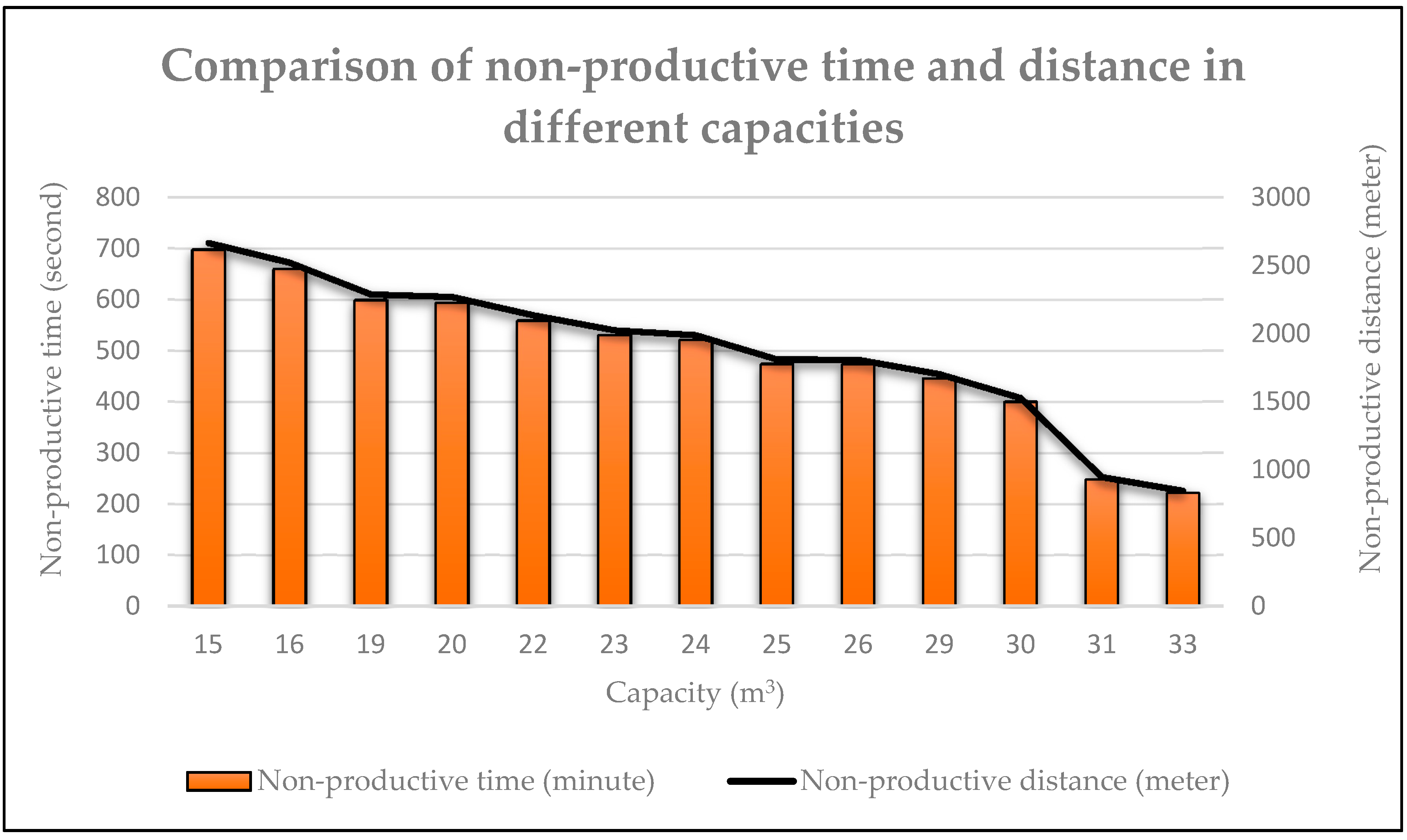
| Capacity of Slurry Tank (L) | Weight (tons) | Non-Productive Time (min) | Non-Productive Distance (m) | Required Tractor’s Power Take Off (PTO) (hp) |
|---|---|---|---|---|
| 15,000 | 18 | 11.6344 | 2667 | 180 |
| 16,000 | 19.2 | 11.002 | 2522 | 200 |
| 19,000 | 22.8 | 9.9852 | 2289 | 240 |
| 20,000 | 24 | 9.9066 | 2271 | 260 |
| 22,000 | 26.4 | 9.3193 | 2136 | 280 |
| 23,000 | 27.6 | 8.841 | 2026 | 300 |
| 24,000 | 28.8 | 8.6836 | 1990 | 300 |
| 25,000 | 30 | 7.9044 | 1812 | 320 |
| 26,000 | 31.2 | 7.8946 | 1809 | 340 |
| 29,000 | 34.8 | 7.433 | 1704 | 380 |
| 30,000 | 36 | 6.6692 | 1529 | 380 |
| 31,000 | 37.2 | 4.1349 | 948 | 400 |
| 33,000 | 39.6 | 3.6942 | 847 | 420 |
| Weight (tons) | Non-Productive Time (min) | Non-Productive Distance (m) | Required Tractor PTO (hp) |
|---|---|---|---|
| 2 | 3 | 4 | 1 |
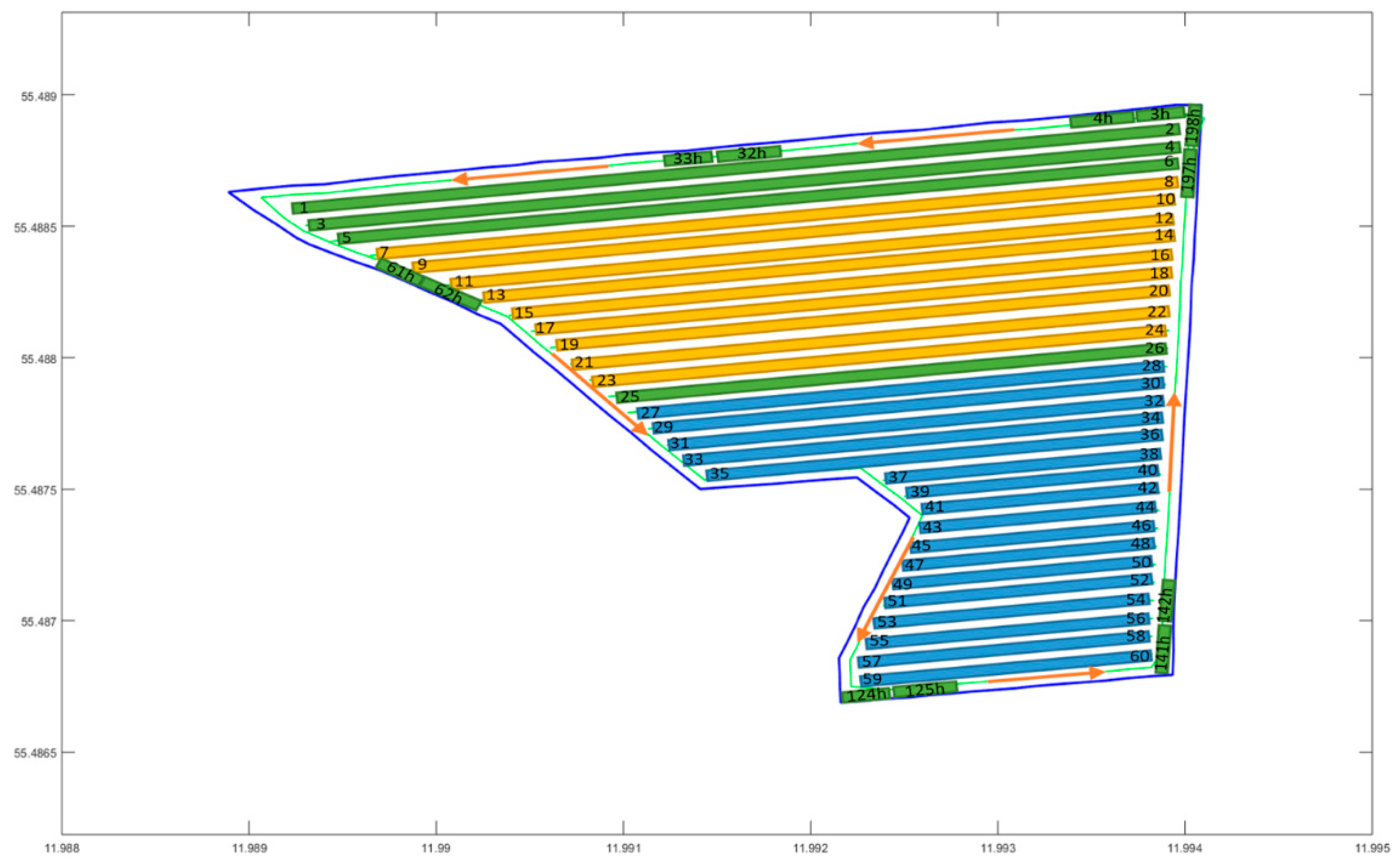
| Location | Working Width (m) | Dosage (t/ha) | Number of Tracks | Turning Radius (m) | |
|---|---|---|---|---|---|
| Latitude: 55°29’19” N Longitude: 11°59’32” E | 25 | 7.5 | 17 | 30 | 9 |
| Optimized Solution | <0, 12, 9, 8, 13, 20, 21, 24, 17, 16, 0, 30, 31, 54, 55, 58, 59, 51, 50, 47, 44, 41, 40, 45, 36, 37, 34, 27, 0, 4, 1, 6, 25, 3 h, 4 h, 5 h, 6 h, 7 h, 8 h, 9 h, 10 h, 11 h, 12 h, 13 h, 14 h, 15 h, …, 198 h, 199 h, 0> |
| Non-Working Distance (m) | 2788 |
© 2020 by the authors. Licensee MDPI, Basel, Switzerland. This article is an open access article distributed under the terms and conditions of the Creative Commons Attribution (CC BY) license (http://creativecommons.org/licenses/by/4.0/).
Share and Cite
Vahdanjoo, M.; Madsen, C.T.; Sørensen, C.G. Novel Route Planning System for Machinery Selection. Case: Slurry Application. AgriEngineering 2020, 2, 408-429. https://doi.org/10.3390/agriengineering2030028
Vahdanjoo M, Madsen CT, Sørensen CG. Novel Route Planning System for Machinery Selection. Case: Slurry Application. AgriEngineering. 2020; 2(3):408-429. https://doi.org/10.3390/agriengineering2030028
Chicago/Turabian StyleVahdanjoo, Mahdi, Christian Toft Madsen, and Claus Grøn Sørensen. 2020. "Novel Route Planning System for Machinery Selection. Case: Slurry Application" AgriEngineering 2, no. 3: 408-429. https://doi.org/10.3390/agriengineering2030028
APA StyleVahdanjoo, M., Madsen, C. T., & Sørensen, C. G. (2020). Novel Route Planning System for Machinery Selection. Case: Slurry Application. AgriEngineering, 2(3), 408-429. https://doi.org/10.3390/agriengineering2030028