3.1. Hardware
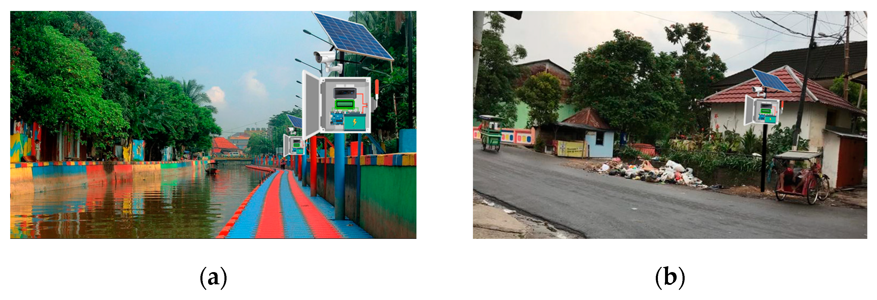
The mechanical design of the monitoring device in this research can be seen in
Figure 3a. It consists of two main parts, namely (1) the solar cell, which includes a solar cell components’ box and a pole; and (2) the electronic monitoring components box. The solar cell component box as shown in
Figure 3b is filled with components, such as: (1) a battery that functions as the power source and the storage of the electric power that has been obtained from the solar cell. This battery has two electrodes that interact with sulfuric acid so that they change into lead sulfate. This produces current flow when the lead electrode lets some electrons free; (2) the SCC or Solar Charger Controller that is used to optimize and to guarantee that the lifetime of the battery can be upgraded. The SCC has 2 important modes, namely charging and operating. In charging mode, the SCC has a responsibility to charge and to maintain the battery so that it is not overcharged, while in the operating mode, the SCC is used to maintain the supply to the load. When the battery is almost empty, the SCC stops the supply; (3) the battery MCB (Miniature Circuit Breaker), which ensures that there is no short circuiting of the battery; (4) the MCB panel that functions as protection and as the guard against the current overload; (5) the MCB inverter that functions as the breaker for the solar panel in order to avoid short circuit and overload; (6) the inverter that converts DC to AC; (7) the LVD (Low Voltage Disconnect) that functions as the battery protection from the over-discharge. It stops the battery load when the battery is low and it automatically connects the battery load when the battery has been charged.
In the electronic monitoring components box (
Figure 3c), the components are placed in two parts, namely the cover and the internal part. In the cover, there are 6 components, including (1) the MQ7 that detects the occurrence of dangerous gases; (2) the DHT22 sensor used to detect the surrounding humidity; (3) the webcam that captures the video; (4) the JSN-SR04 ultrasonic sensor that detects the Sekanak River water level; (5) the speaker that notifies people who litter; (6) the LCD that displays the data regarding the temperature, humidity, air quality, and water level. Meanwhile, in the internal part, there are components, including (1) the PC fan that ensures the mini PC remains at its normal temperature; (2) the Arduino Uno microcontroller that functions as the controller of the environmental sensors used in this research; (3) the mini breadboard that functions as the connector of the connecting cables; (4) the mini PC that functions as the signal processor. It has responsibility to send the obtained data to the router; (5) the router-modem that functions as the channel that sends and receives the data; (6) the volume controller that controls the produced voices.
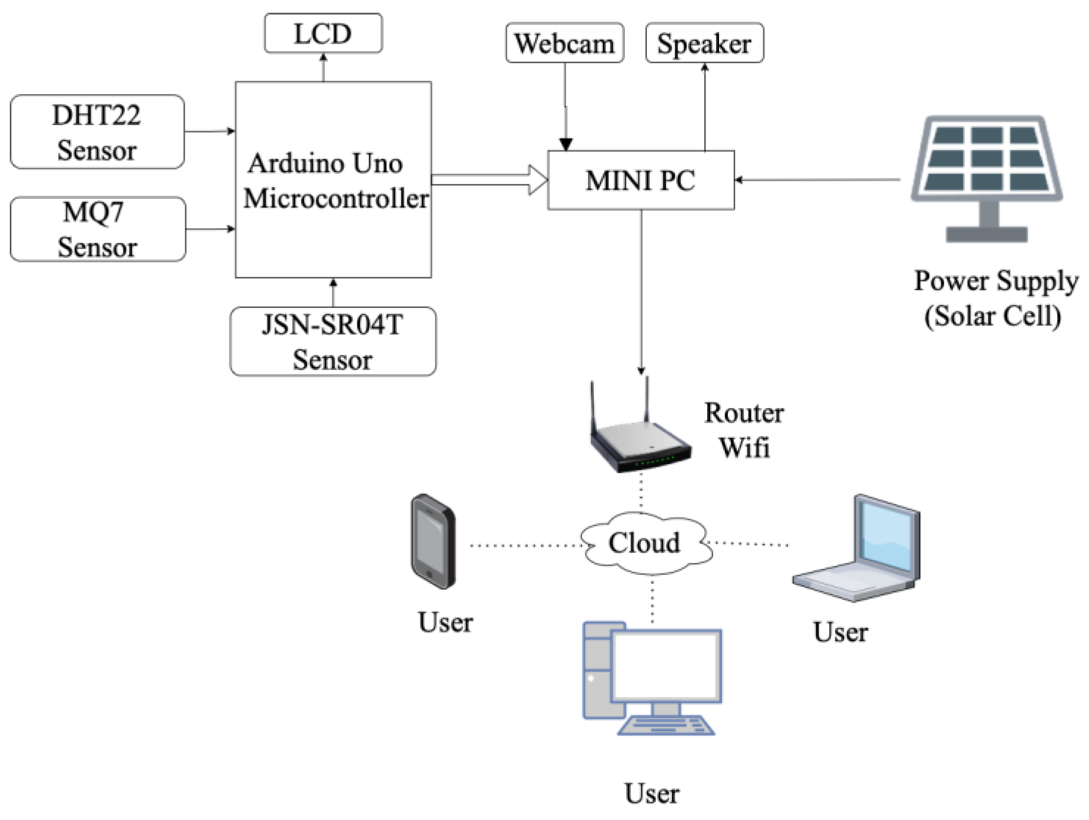
The block diagrams of the monitoring systems can be seen in
Figure 4. Overall, the systems applied in the Sekanak River and mini garden consist of the same connection, as shown in
Figure 4. However, the monitoring system in the mini garden has no waterproof ultrasonic sensor, as applied in the Sekanak River monitoring system. The power supply obtained from the solar cell is input into the Mini PC that connects to the Arduino and the webcam, which become the input for the Mini PC. The Arduino is the processor of the inputted sensors’ data, i.e., from the Ultrasonic sensor, DHT 22, and MQ7. The data that have been processed by the Arduino is displayed on the LCD and sent to the Mini PC. On the other side, the webcam that captures the human activity near it is also has a connection to the mini-PC. The video captured by the webcam is processed by the mini-PC and then is sent to the cloud server through the Wi-Fi router which, then sends the final data to the users. The users can use their mobile phone, PC, or laptop to monitor the littering activity.
3.2. Software
In this research, there were two methods used, i.e., the first using CNN only and the second using CNN-LSTM. The architecture of the CNN can be seen in
Figure 5, while the CNN LSTM is presented in
Figure 6.
The architecture of the CNN shown in
Figure 5 consists of 3 main parts, i.e., (1) preparation, (2) feature learning, and (3) classification. The preparation includes inputting the video, conducting the data pre-processing, transferring the video into images, dividing the datasets, and preparing the CNN model. The process is continued to the feature learning, where the pooling is conducted between convolution 1 and convolution 2. After that the classification takes place. In this stage, the data obtained from the pre-processing process are flattened, dropped out, densified, and passed through the fully connected layer so that they can decide what activity is being performed.
In this research, videos that have been collected from two places, i.e., Sekanak River and the mini garden are processed in the data pre-processing. In this process, all video data enter the video extraction stage in which the video is extracted into several images. Videos that have durations up to 5 min are split into 173 jpg images with jpeg format RGB size 427 × 240, 22.3 kb. Then, the video extraction results are placed in 2 prepared folders, namely the littering and normal folders. The system adds up all the images results that can be solved by the system. After the image is obtained from the video extractor, the image is separated. After that, the data enter the CNN model process, during which they enter the learning features process. In this process, the input that is ready to become a CNN model performs a convolution stage for 1 layer with a 3 × 3 kernel and 64 filter. This network activates the sigmoid at each layer. After that, the data are pooled 2 × 2 and continued to the second convolution using the kernel or filter sigmoid of size 128, 3 × 3. Then, they enter the classification process, starting from the flattening process.
When a flat layer is formed, the vector value of 128 channels, size 3 × 3 is converted into a single vector form. After the multiplication of 3 × 3 × 128 is calculated, there will be 1152 values that will enter the neural network. After the process has finished, it is continued to create a solid layer that is set to be 256 units. The resulting vector of 1152 values is entered one by one into 256 units. Thus, it will give (1152 × 256) + 256 bias = 295,168 parameters. After that, the process is continued to the dropout process. It aims to prevent overfitting and to speed up the learning process. The system then temporarily removes the hidden neurons that have probability value between 0 and 1. The dropout for the previous 256 units is redecorated for the solid layer. Thus, the parameters to be generated are (256 × 2) + 2 bias = 514 parameters. Thus, the total parameters performed by Machine Learning are 295,168. After the calculation is completed, it continues to a dense stage, in which, it is provided by adding a fully connected layer so that the data can be classified. The output is the information regarding normal or littering activity.
For the second method, a hybrid of a Convolutional Neural Network (CNN) and Long Short-Term Memory (LSTM) was used as the intelligence for detecting the littering activity. In
Figure 6, data preparation is carried out. Then, the process is continued with inputting the video. After that, it enters the process of the transferring video into images. Each video produces 173 RGB 427 × 240 jpeg images, 22.3 kb. Then, the video extraction results are saved into the provided folders, namely littering and normal folders. After that, the system prepares the Resnet, which is a classical neural network. Then, the data enter the feature learning stage process to determine the characteristics of each image that has been solved by the system. The convolution was conducted 5 times to obtain the best results. In this convolution process, every time the system convolutes the data, max-pooling is carried out to retrieve the largest image data. Then, the convolution is carried out again with different sizes. At the end of the convolution, average pooling is carried out, i.e., by calculating the average value of the feature patch obtained. Then, the data can be fully connected so that they become the input of the LSTM (long short-term memory) process. In this process the data are sorted by following the old context on the LSTM with the new context. Then, the data are divided into 2, namely training data and testing data. After that, the system prepares an optimization process and the data are assessed by the class system classifier.
Using CNN-LSTM, the researchers can obtain information from the entire scale of objects so that they can classify objects more accurately. The steps that should be conducted in this research can be described as follows:
Dataset preparations were obtained by collecting videos of littering activity and non-littering activity. There were 400 videos that consisted of 200 videos for littering and 200 videos for non-littering activities. The non-littering activities in this research were categorized as normal activities.
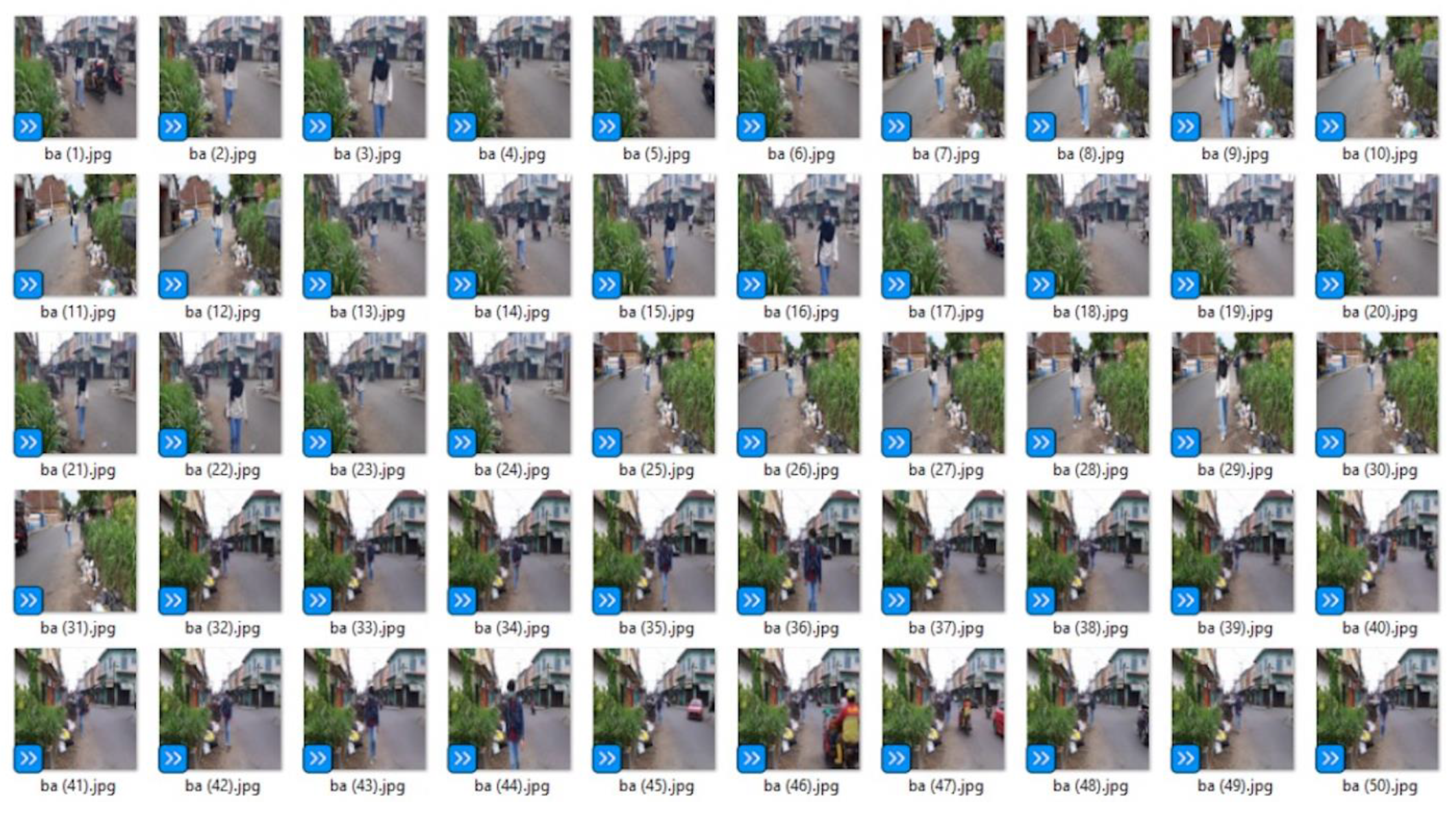
Transferring the videos into images.
The next step was to transfer the video into images. Each video obtained in the data preparation was then converted into about 100–300 images as shown in
Figure 7.
The datasets were then divided into the testing data and training data. In this research, the tests data size was 0.2 and the training data size was 0.8.
The model used was Restnet 101 [
33], in which the model used was the Residual CNN for classifying the images obtained before. In Restnet 101, there are 101 layers that are divided into 3-layer blocks. The specification of the architecture layer can be seen in
Table 2. ResNet works by inserting the shortcut connection so that the network becomes the version of the counterpart residue. When the input and the output of the networks are in the same dimension, then the identity shortcut,
, can be directly used. However, when the shortcut is different, the system makes the system become identical by increasing the dimension using extra zero entries or the projection shortcut in
is used in order to match dimensions using 1 × 1 convolution.
In this research, one fully connected layer was set up, in which this layer has 1000 neurons. This fully connected layer has predicted the next image.
The LSTM was designed using 300 inputs, 256 hidden sizes, and 3 layers blocks.
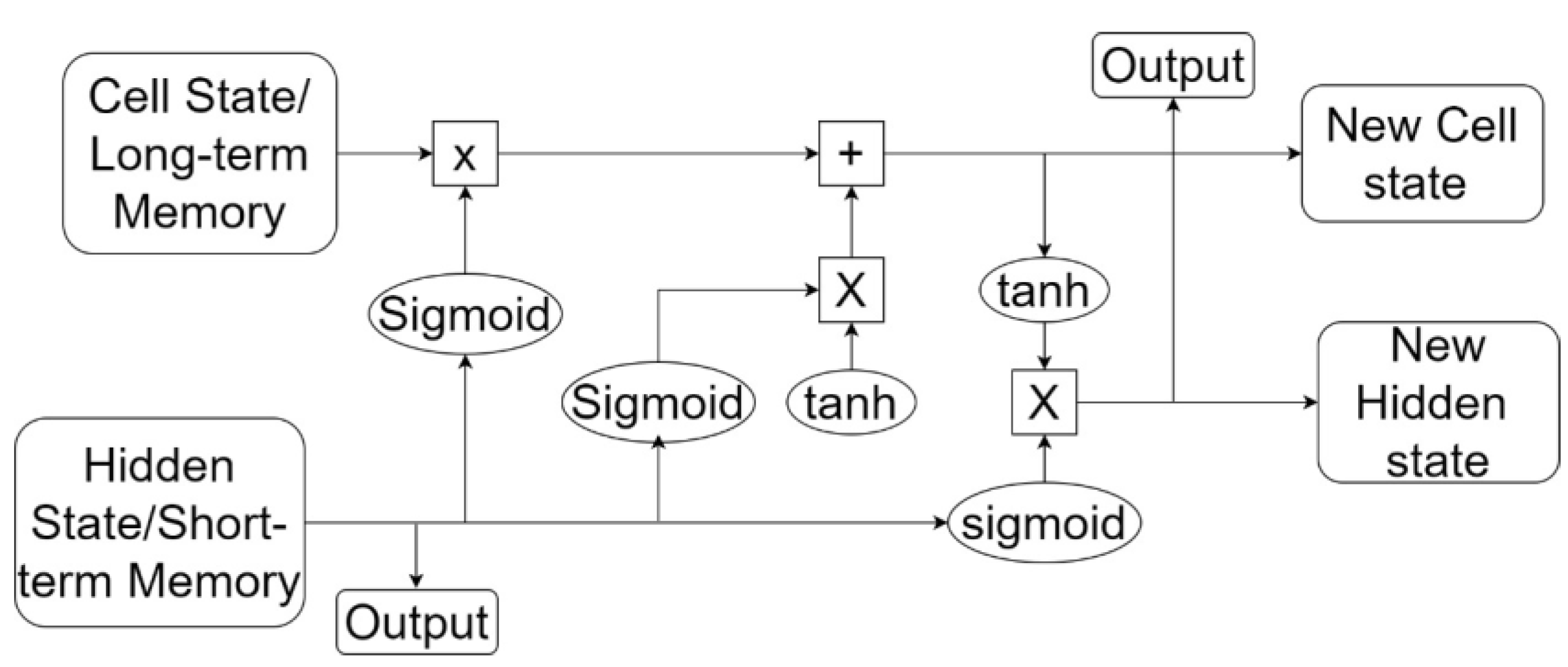
The LSTM architecture used in this research can be seen in
Figure 8. The equations used for each element in the sequence are as follows:
where:
is the hidden state at the time ;
is the cell state at the time ;
is the input at the time ;
is the hidden state at the time ;
are the input, forget, cell, and output gate;
is the sigmoid function;
is the Hadamard product.
The loader used was a data loader from pytorch and is intended for preparation of the data so that they are ready to be trained and tested. The most important thing in this set-up is the dataset that will be processed. In this research, the video that is converted to the pictures becomes the dataset. This dataset is then processed using an iterable-style dataset.
The optimizer used in this research is torch.optim. It accelerates the training and testing process so that they can achieve the effective value quickly. The optimizer object used holds the current state and updates parameters.
This criterion determination is useful in balancing the training set that is used. The input for this step is the raw data and the target of the criterion is in the class indices of the range , where is the number of the class.
Figure 8 below shows the architecture of the LSTM. In
Figure 8, the data that have been prepared and have passed through the CNN process are input into the LSTM process. The data are connected to the cell state/long-term memory at the top of the LSTM module. The system performs multiplication and addition operations so that the data become a new cell state. This initial process is assisted by the existence of a sigmoid gate which regulates how much information can pass. Then, the system decides which information can pass after obtaining a new cell state. At this stage, there are 2 parts, namely the sigmoid gate which first decides which value to be updated. Then, the tanh layer generates a new context vector candidate, or a new cell state vector candidate. After that, it combine the two and update the context again. The next step is to update the old context or long-term memory to the new cell state by multiplying the new cell state by sigmoid to determine how many candidates the system will include in the new context. Then, the system adds up the long-term memory with the new cell state. The output value obtained at this stage is based on the context value that has been passed to a filter. The first thing is that the system runs a sigmoid gate to determine which parts of the context the system generates. Then, the system passes through the tanh layer to make the values −1 and 1. At the end, the system is multiplied by the sigmoid gate output so that the system determines the part that can be disconnected.


 ,
, 


