Article

A Markov Switching Autoregressive Model with Time-Varying Parameters

1
Department of Statistics, Faculty of Science and Data Analytics, Institut Teknologi Sepuluh Nopember, Surabaya 60111, Indonesia
2
Department of Statistics, Faculty of Mathematics and Natural Sciences, Universitas Negeri Yogyakarta, Yogyakarta 55281, Indonesia
*
Author to whom correspondence should be addressed.
Forecasting 2024, 6(3), 568-590; https://doi.org/10.3390/forecast6030031
Submission received: 23 May 2024 / Revised: 22 July 2024 / Accepted: 26 July 2024 / Published: 29 July 2024

Abstract

:
This study showcased the Markov switching autoregressive model with time-varying parameters (MSAR-TVP) for modeling nonlinear time series with structural changes. This model enhances the MSAR framework by allowing dynamic parameter adjustments over time. Parameter estimation uses maximum likelihood estimation (MLE) enhanced by the Kim filter, which integrates the Kalman filter, Hamilton filter, and Kim collapsing, further refined by the Nelder–Mead optimization technique. The model was evaluated using U.S. real gross national product (GNP) data in both in-sample and out-of-sample contexts, as well as an extended dataset to demonstrate its forecasting effectiveness. The results show that the MSAR-TVP model improves forecasting accuracy, outperforming the traditional MSAR model for real GNP. It consistently excels in forecasting error metrics, achieving lower mean absolute percentage error (MAPE) and mean absolute error (MAE) values, indicating superior predictive precision. The model demonstrated robustness and accuracy in predicting future economic trends, confirming its utility in various forecasting applications. These findings have significant implications for sustainable economic growth, highlighting the importance of advanced forecasting models for informed economic policy and strategic planning.

1. Introduction

Various approaches have been proposed to model the time series of real GNP, aiming to characterize long-term trends and their relationships with business cycles. Our focus is on modeling nonlinear time series that undergo structural changes, as well as addressing the issue of non-stationarity, which is common in economic data. Nonlinear time series data are types of data that do not follow linear patterns or functions, meaning the relationships between variables are unstable and can change over time. Structural changes refer to shifts in patterns that occur within the time series data. Linear time series models, such as the autoregressive integrated moving average (ARIMA), typically cannot capture the nonlinear patterns in data [1,2]. Consequently, time series models have been continuously developed to handle nonlinearity and accommodate structural changes.
One well-known approach is the Markov switching (MS) model, developed by Hamilton [3], and its combination with the autoregressive (AR) model is referred to as the Markov switching autoregressive (MSAR) model. This model is designed to address structural changes resulting from data shifts over certain periods, a significant advancement from the traditional linear AR model described in [4,5]. MSAR divides data into several regimes, each of which follows its own AR model. The fundamental idea of this model is to dynamically adapt to changes in data patterns. These changes are influenced by a discrete, unobserved random variable referred to as a state or regime. By considering these unobserved regimes, the model facilitates transitions between those with predetermined probabilities. This approach effectively captures the non-stationarity of the distribution by introducing switches that reflect changes in not only hidden but also observed data.
The MSAR model has attracted considerable attention for its ability to analyze complex dynamics, including asymmetry and conditional heteroskedasticity, which can be readily estimated and interpreted [6]. Extensive studies have fostered the development of this model across various extensions, and its application extends to a wide range of disciplines, especially within economics and finance [3,7,8,9,10,11]. Among the developments of the MSAR model is the MS model with autoregressive conditional heteroskedasticity (ARCH), which excels in handling long-term regime changes and short-term variability in time series data [12,13]. Some researchers have, furthermore, developed time series models incorporating flexible parameter movements, such as the MS model with time-varying transition probabilities (MS-TVTP) [14], which has proven effective in explaining data movements. Another development is an MS model with a mixture distribution that does not require Gaussian white noise residuals [15].
In addition, another approach used to address non-stationarity is the time-varying parameter (TVP) model. The TVP model is a time series model with parameters that vary over time [16]. It can be considered a special case of the state-space model. This model handles structural changes that evolve over time. In its implementation, the TVP model allows parameters within the model to change over time, making it more flexible in modeling complex non-stationary time series data compared to the MSAR model [17]. Based on the state-space framework initially introduced by Kalman [18], the TVP model employs the Kalman filter algorithm for parameter estimation. Studies on the Kalman filter and TVP models show that state-space models can represent unobserved variables and forecast multiple interconnected time series with dynamic interactions [19,20,21]. In the TVP model, the time-varying parameters are unobserved random variables that must be estimated using the observed data.
Considering the flexibility of state-space models and the capability of MS models to capture structural changes, several researchers have developed state-space models with Markov switching [22,23]. These models effectively handle dynamic changes in time series data structures by accommodating transitions between different regimes. This approach is highly flexible and allows for the estimation of various model classes that were previously difficult to perform. It has been further extended to include Markov switching heteroskedasticity [24]. The principle of these models is to consider unobserved state vectors that include not only switching variables but also other variables in the model.
Apart from these advancements, several studies have explored the use of triplet Markov models (TMMs) to address similar issues in time series data. Meanwhile, other studies [25] have developed deep parameterizations for pairwise and TMMs relevant to the unsupervised classification of sequential data, highlighting advancements in handling non-stationary parameters similar to the state-space with Markov switching models. Other research [26] introduced a non-stationary normalized difference vegetation index (NDVI) time series modeling using triplet Markov chains, demonstrating the effectiveness of TMMs in capturing time-varying dynamics. Further studies [27] discussed optimal recursive filtering and smoothing in non-Gaussian MS models, providing insights into the complexity of parameter estimation in similar models. Additionally, other work [28] presented an application of TMMs for modeling consumer loan repayment behavior across business cycles, illustrating the practical relevance of TMMs in financial contexts. Nonetheless, it is crucial to recognize that these studies, along with previously mentioned MSAR and state-space models, have mainly concentrated on monitoring and analyzing current data rather than extending their application to forecasting. This reveals a notable gap in the literature that our research seeks to fill by utilizing such models for economic forecasting.
Considering the greater flexibility of the TVP model in modeling complex time series data, and the MSAR model’s strength in depicting nonlinear time series data by dividing it into multiple regimes, we developed a novel approach in this study. This new approach termed the Markov switching autoregressive model with time-varying parameters (MSAR-TVP) enhances the existing MSAR framework by integrating parameters that vary over time within each regime. Our model accounts for switching in the mean, AR coefficients, and error variance, with parameters assumed to follow an AR process that changes depending on the regime.
The main goal of this study was to develop and validate the effectiveness of the MSAR-TVP, an advanced method for analyzing and forecasting nonlinear time series data that underwent structural changes. This model was designed to enhance prediction accuracy by dynamically adjusting to new information and structural changes in economic data. Its specifications, suitable for nonlinear time series data that underwent stochastic structural changes, could handle complex data, which are typically difficult to explain with linear or nonlinear models with fixed parameters.
The MSAR-TVP model integrates the robustness of the MS framework with the flexibility of time-varying parameters, enhancing the accuracy of data behavior predictions. By leveraging the dynamics of regime changes, this model can estimate parameters associated with each regime and identify changes in the transition probability matrix. This approach provides more precise predictions of the behavior of nonlinear time series undergoing structural changes.
To validate the proposed MSAR-TVP model, we developed a parameter estimation methodology using maximum likelihood estimation (MLE), combined with the Kim filter, which integrates the Kalman filter, Hamilton filter, and Kim collapsing. Kim’s filtering scheme, which simplifies the information set for state-space models, enhances computational efficiency [22,23,29]. The optimization of parameters was performed using the Nelder–Mead method, a technique for finding local minima without relying on function derivatives. This method has been effective in situations where derivatives of the objective function are difficult to determine or compute [30,31,32]. The reliability and precision of the MSAR-TVP model were confirmed by measuring the mean absolute percentage error (MAPE) and mean absolute error (MAE).
This study implemented the MSAR-TVP model on U.S. real GNP data, using Q3 1952 to Q4 1984 as in-sample data and Q1 1985 to Q4 1986 as out-of-sample data to evaluate its forecasting performance compared to the traditional MSAR model. Additionally, the model was applied to an extended dataset from Q1 1947 to Q1 2024 to demonstrate its forecasting effectiveness. The results show that the MSAR-TVP model improves forecasting accuracy, achieving lower MAPE and MAE values, and indicating superior predictive precision. The research also explored the model’s performance in detecting the duration of each state using average run length (ARL).
The application of this model to real GNP data provides new insights into the dynamics of economic growth. It utilizes an approach that adapts to rapid and significant economic changes, which is crucial for achieving sustainable economic growth. This adaptability enables models to respond to both short-term fluctuations and long-term structural shifts in the economy.
This research makes a significant contribution to the econometric forecasting literature by developing the MSAR-TVP model, designed to address non-stationarity and regime shifts in economic time series. By using the Nelder–Mead approach and the Kim filter, this model integrates efficient estimation techniques. It also allowed for dynamic parameter adjustments in response to new data and structural changes, thus ensuring more accurate and reliable predictions. In addition, this study also applied the MSAR-TVP model in forecasting economic data. The results of this study can not only enrich the academic literature but also provide a valuable practical tool for forecasters and policymakers to address complex economic challenges.
This paper is structured as follows: Section 2 provides an overview of the fundamental model, delineates the development of the MSAR-TVP model, and explains the creation of the parameter estimation technique. Section 3 presents the results. Section 4 discusses the empirical findings and suggests future research directions. Finally, Section 5 concludes the paper by summarizing the results.

2. Materials and Methods

2.1. State-Space Model

The state-space model, initially developed by Kalman [18], is essential for illustrating the dynamics of systems characterized by unobservable state variables [21,33,34]. The fundamental composition of this model comprises two main equations: first, the measurement equation, also known as the observation equation, and second, the transition equation, often referred to as the state equation. The measurement equation links the observed data with the unobservable state variables, while the transition equation describes the evolution of these state variables over time. The state-space model is defined as follows:
y t = H t β t + A z t + ε t ,
β t = δ * + F β t 1 + ν t ,
where y t is the dependent variable at time t , for t = 1 , 2 , , T ; β t is a vector of unobserved state variables at time t , sized p × 1 ; H t is the measurement matrix at time t that connects the state vector β t with the observed measurement y t , sized T × p ; z t is an observed exogenous variable, sized r × 1 ; A is the matrix linking the exogenous variable z t with the observed measurement y t , sized T × r ; δ * is a constant vector, sized p × 1 ; β t 1 is the state vector at time t 1 , sized p × 1 ; F is a matrix whose elements can be data on the exogenous variable or constant parameters, sized p × p ; ε t is the error term of the measurement equation, with ε t ~ i . i . d . N ( 0 , σ 2 ) ; ν t is the error term vector of the transition equation, with ν t ~ i . i . d . N ( 0 , Q ) ; σ 2 is the variance of ε t ; and Q is the covariance matrix of ν t , sized p × p .

2.2. Time-Varying Parameter Model

The time-varying parameter (TVP) model, a specialized form of univariate time series models with parameters that vary over time, is part of the state-space models framework [16,18]. In this particular model, the matrix H t in Equation (1) is substituted with x t , which is a vector of explanatory variables, either exogenous or predetermined. Concurrently, β t represents the time-varying parameters, indicative of structural changes occurring over time. Within this model, it is assumed that these parameters follow a first-order AR process. The formulation of the TVP model is as follows:
y t = x t β t + ε t , ε t ~ i . i . d . N ( 0 , σ 2 ) ,
β t = δ * + F β t 1 + ν t , ν t ~ i . i . d . N ( 0 , Q ) .
Here, each component within the error term vector ν t is assumed to be mutually independent. Furthermore, the entire vector ν t operates independently from the error term ε t . Equation (3) serves as the measurement equation allowing for time-varying parameters, while Equation (4), the parameter transition equation, determines the movement of these parameters over time. In this research, the term “parameter transition equation” is used for the TVP model to emphasize that β t represents time-varying parameters.
In the TVP model, the explanatory variable x t can be an exogenous or a predetermined variable. A predetermined variable’s value is established in advance, functioning either as an exogenous factor or as a lag of an endogenous variable [35]. A specific variant of the TVP model, where x t is an endogenous lag variable represented as x t = y t 1 y t 2 y t p , is known as the time-varying coefficient autoregressive (TVAR) model. Essentially, the TVAR model is an AR model characterized by time-varying coefficients or parameters [23,36,37,38]. The TVAR model assumes that the error term ε t follows an i.i.d. normal distribution, ε t ~ i . i . d . N ( 0 , σ 2 ) , and the error term in the parameter transition equation ν t , k also follows an i.i.d. normal distribution, ν t , k ~ i . i . d . N ( 0 , σ k 2 ) . These assumptions are also known as a Gaussian white noise process [33].
The equation of the TVAR model, where the time-varying parameters follow an AR(1) process, can be written as follows [38]:
y t = β t , 1 y t 1 + β t , 2 y t 2 + + β t , p y t p + ε t , ε t ~ i . i . d . N ( 0 , σ 2 ) ,
β t , k = ϕ k β t 1 , k + ν t , k , ν t , k ~ i . i . d . N ( 0 , σ k 2 ) , k = 1 , 2 , , p ,
where y t is the dependent variable at time t ; β t , k is the time-varying coefficient of the k -th order AR at time t ; y t k is the endogenous lag variable of y t ; and ϕ k is the AR coefficient of the k -th order in the parameter transition equation.
It should be noted that in Equations (5) and (6), the TVAR model does not include a constant or intercept. This approach is appropriate for cases where the time series is assumed to be stationary with a zero mean, suggesting that the model relies solely on previous lag values y t k and the error term ε t . This characteristic makes the TVAR model particularly suitable for data centered around zero or in situations where assuming a negligible long-term mean is justified.

2.3. Markov Switching Autoregressive Model

The Markov switching (MS) model is a sophisticated nonlinear time series model designed to address structural changes within data. This model is strategically crafted to adapt dynamically to changes in data patterns, which are impacted by an unobserved discrete random variable, S t , often labeled as the state or regime. S t is assumed to follow a first-order Markov chain, where the value of a state at any given period depends solely on the value of its immediately preceding state. It can take values of { 1 , 2 , , M } with M representing the total number of states.
As defined by Hamilton, the MS model is described as follows [7,33,39]:
y t = μ S t + ε t ,
where y t is the dependent variable at time t ; μ S t is the mean at time t of the observed data, influenced by state changes; ε t is the error term at time t with ε t ~ i . i . d . N ( 0 , σ S t 2 ) ; and σ S t 2 is the variance of ε t , influenced by state changes. To capture the essential property of the Markov chain in an M -state, first-order Markov process, the transition probability matrix can be written as:
P = p 11 p 12 p 1 M p 21 p 22 p 2 M p M 1 p M 2 p M M ,
where p i j = P ( S t = j S t 1 = i ) with j = 1 M p i j = 1 for all i = 1 , 2 , , M , and 0 p i j 1 . These p i j values delineate the probability of transitioning from state i to state j , underlining the crucial role of this matrix in defining possible state transitions and their probabilities.
One of the simplest forms of integrating the MS model with another time series model is the Markov switching autoregressive (MSAR) model. Assuming that y t follows an AR model of order p , the formulation of the MS model combined with AR of order p , for M regimes, is referred to as MS ( M ) AR ( p ) . The model is described as follows [7,9,33,40]:
( y t μ S t ) = ϕ 1 , S t ( y t 1 μ S t 1 ) + + ϕ p , S t ( y t p μ S t p ) + ε t , ε t ~ i . i . d . N ( 0 , σ S t 2 ) ,
where y t k is the endogenous lag variable of y t with k = 1 , 2 , , p ; μ S t k is the mean at time t k , influenced by state changes; and ϕ k , S t is the AR coefficient of the k -th order. The transition probability matrix for the MSAR model is as shown in Equation (8). The means μ S t and the variance of error σ S t 2 are defined as follows:
μ S t = μ 1 S t , 1 + μ 2 S t , 2 + + μ M S t , M ,
σ S t 2 = σ 1 2 S t , 1 + σ 2 2 S t , 2 + + σ M 2 S t , M ,
where S t , j is a dummy variable that equals 1 if the current state S t matches state j , and 0 otherwise.
Furthermore, Equation (9) can also be reformulated as:
y t = c S t + ϕ 1 , S t y t 1 + ϕ 2 , S t y t 2 + + ϕ p , S t y t p + ε t ,
where c S t = μ S t ϕ 1 , S t μ S t 1 ϕ p , S t μ S t p and acts as the model’s constant or intercept.
The model could then be used in this study.

2.4. Markov Switching Autoregressive Model with Time-Varying Parameters

This study proposed an extension of the MSAR model, referred to as the Markov switching autoregressive model with time-varying parameters (MSAR-TVP). This model combines the MS framework with an AR model incorporating time-varying dynamics. The concept expands the MSAR into a state-space model representation, integrating time-varying parameters as specific time functions, aligned with the AR(1) process.
The development of the MSAR-TVP model involves adopting the MS ( M ) AR ( p ) configuration within the MSAR framework, indicating M regimes, with each regime’s process adhering to an AR ( p ) pattern. The model’s time-varying parameters are denoted as β t , k , S t for each k = 1 , 2 , , p ,   S t { 1 , 2 , , M } , and t = 1 , 2 , , T . These parameters follow an AR(1) process.
Using the state-space model representation, the MSAR-TVP model equations can be defined as follows:
Measurement Equation:
( y t μ S t ) = β t , 1 , S t ( y t 1 μ S t 1 ) + + β t , p , S t ( y t p μ S t p ) + ε t ,
Parameter Transition Equation:
( β t , k , S t δ k , S t ) = ϕ k , S t ( β t 1 , k , S t δ k , S t 1 ) + ν t , k , k = 1 , 2 , , p ,
where y t is the dependent variable at time t ; y t k is the explanatory variable comprising the endogenous lag of y t ; μ S t is the mean at time t of the observed data, influenced by state changes; μ S t k is the mean at time t k of the observed data, influenced by state changes; β t , k , S t is the unknown time-varying parameter of the k -th order AR at time t , influenced by state changes; ϕ k , S t is the k -th order AR coefficient in the parameter transition equation, influenced by state changes; δ k , S t is the mean at time t in the k -th order AR in the parameter transition equation, influenced by state changes; δ k , S t 1 is the mean at time t 1 in the k -th order AR in the parameter transition equation, influenced by state changes; ε t is the error term of the measurement equation, with ε t ~ i . i . d . N ( 0 , σ S t 2 ) ; ν t , k is the error term of the parameter transition equation, with ν t , k ~ i . i . d . N ( 0 , σ k , S t 2 ) ; σ S t 2 is the variance of ε t , influenced by state changes; and σ k , S t 2 is the variance of ν t , k , influenced by state changes.
In the MSAR-TVP model, as delineated by Equations (13) and (14), each parameter is contingent upon the subscript S t , which indicates the state variable. The random variable S t takes discrete values S t { 1 , 2 , , M } . The transition probabilities from one state to another are denoted by p i j , where p i j = P ( S t = j S t 1 = i ) with j = 1 M p i j = 1 for all i = 1 , 2 , , M , and 0 p i j 1 . These transition probabilities can be represented in the transition probability matrix as defined in Equation (8).
Based on Equations (13) and (14), the MSAR-TVP model is articulated in matrix form as follows:
Measurement Equation:
y t = μ S t * + y t 1 y t 2 y t p β t , 1 , S t β t , 2 , S t β t , p , S t + ε t ,
where μ S t * = μ S t β t , 1 , S t μ S t 1 β t , 2 , S t μ S t 2 β t , p , S t μ S t p and ε t ~ i . i . d . N ( 0 , σ S t 2 ) ,
Parameter Transition Equation:
β t , 1 , S t β t , 2 , S t β t , p , S t = δ 1 , S t * δ 2 , S t * δ p , S t * + ϕ 1 , S t 0 0 0 ϕ 2 , S t 0 0 0 ϕ p , S t β t 1 , 1 , S t β t 1 , 2 , S t β t 1 , p , S t + ν t , 1 ν t , 2 ν t , p ,
where δ k , S t * = δ k , S t ϕ k , S t δ k , S t 1 and ν t , k i . i . d . N ( 0 , σ k , S t 2 ) for each k = 1 , 2 , , p .
Furthermore, based on Equations (15) and (16), we define h t = y t 1 y t 2 y t p ,   β t , S t = β t , 1 , S t β t , 2 , S t β t , p , S t ,   δ S t * = δ 1 , S t * δ 2 , S t * δ p , S t * ,   F S t = ϕ 1 , S t 0 0 ϕ p , S t ,   β t 1 , S t = β t 1 , 1 , S t β t 1 , 2 , S t β t 1 , p , S t ,   and   ν t = ν t , 1 ν t , 2 ν t , p . The general state-space representation of the MSAR-TVP model can be expressed in vector and matrix notation as follows:
y t = μ S t * + h t β t , S t + ε t ,
β t , S t = δ S t * + F S t β t 1 , S t + ν t ,
and the transition probabilities from one state to another, denoted by p i j , are represented in the transition probability matrix as shown in Equation (8).

2.5. Estimation Procedures

This section describes the parameter estimation process for the MSAR-TVP model, using a method based on the Kim filter algorithm. Originally introduced by Kim [22], this algorithm was adapted in this study for the MSAR-TVP model. The approach integrates MLE with the Kalman and Hamilton filters to address the challenges posed by unobserved state vectors. In the MSAR-TVP model, the state vector comprises time-varying parameters that indicate changes in state or regime within the model.
This research formulated the parameter estimation algorithm for the MSAR-TVP model, considering the state-space representation in Equations (17) and (18). The focus was on cases where the AR order was p = 1 and the number of regimes was M = 2 , denoted as MS(2)-AR(1)-TVP. The model equations are given as follows:
y t = μ S t * + y t 1 β t , 1 , S t + ε t , ε t ~ i . i . d . N ( 0 , σ S t 2 ) ,
β t , 1 , S t = δ 1 , S t * + ϕ 1 , S t β t 1 , 1 , S t + ν t , 1 ,   ν t , 1 ~ i . i . d . N ( 0 , σ 1 , S t 2 ) ,
where μ S t * = μ S t β t , 1 , S t μ S t 1 and δ 1 , S t * = δ 1 , S t ϕ 1 , S t δ 1 , S t 1 . Meanwhile, the transition probability matrix is the same as in Equation (8) with M = 2 , and is given as follows:
P = p 11 p 12 p 21 p 22 ,
where p i j = P [ S t = j S t 1 = i ] ,   0 p i j 1 , and j = 1 2 p i j = 1 ,   i = 1 , 2 .
The system defined by Equations (19) and (20) is elaborated as follows:
For S t = 1 :
y t = μ 1 * + y t 1 β t , 1 , 1 + ε t , ε t ~ i . i . d . N ( 0 , σ 1 2 ) ,
β t , 1 , 1 = δ 1 , 1 * + ϕ 1 , 1 β t - 1 , 1 , 1 + ν t , 1 ,   ν t , 1 ~ i . i . d . N ( 0 , σ 1 , 1 2 ) ,
where μ 1 * = ( 1 β t , 1 , 1 ) μ 1 and δ 1 , 1 * = ( 1 ϕ 1 , 1 ) δ 1 , 1 ,
For S t = 2 :
y t = μ 2 * + y t 1 β t , 1 , 2 + ε t , ε t ~ i . i . d . N ( 0 , σ 2 2 ) ,
β t , 1 , 2 = δ 1 , 2 * + ϕ 1 , 2 β t 1 , 1 , 2 + ν t , 1 ,   ν t , 1 ~ i . i . d . N ( 0 , σ 1 , 2 2 ) ,
where μ 2 * = ( 1 β t , 1 , 2 ) μ 2 and δ 1 , 2 * = ( 1 ϕ 1 , 2 ) δ 1 , 2 .
For p = 1 and M = 2 , at S t = 1 , the model represents an AR(1) with time-varying parameters in State 1, while at S t = 2 , it represents an AR(1) with time-varying parameters in State 2. Therefore, the MSAR-TVP model can be considered a dynamically time-varying AR(1) model with parameters influenced by state changes S t , with S t { 1 , 2 } .
In the MS(2)-AR(1)-TVP model, there is one time-varying parameter β t for each regime S t = 1 , 2 . Classical approach parameter estimation using the Kim filter algorithm aims to form predictions of the time-varying parameter β t based not only on Y t 1 but also on the random variables S t = j and S t 1 = i . Suppose Y t 1 is the set of past information from the observed data up to time t 1 . The parameter estimation β t based on Y t 1 , with S t = j and S t 1 = i , denoted as β t | t 1 ( i , j ) , can be formulated as follows:
β t | t 1 ( i , j ) = E [ β t Y t 1 , S t = j , S t 1 = i ] .
The estimation of the parameter yields a set of predictions totaling M 2 for each time t , corresponding to every possible value of i and j . Related to these predictions, there are M 2 different variances. The variance of β t | t 1 ( i , j ) , conditional on S t = j and S t 1 = i , and denoted as w t | t 1 ( i , j ) , can be formulated as follows:
w t | t 1 ( i , j ) = E [ ( β t β t | t 1 ) 2 Y t 1 , S t = j , S t 1 = i ] .
Here, β t is the time-varying parameter at time t , and β t | t 1 is the prediction of this parameter at time t based on information up to time t 1 .
The Kim filter algorithm is modified to estimate the parameters of the MSAR-TVP model. This algorithm is a combination of the Kalman filter, Hamilton filter, and Kim collapsing algorithms.

2.5.1. Kalman Filtering

The regime-dependent Kalman filter is used to estimate the time-varying parameters β t for each i , j of the MSAR-TVP model. Conditional on S t 1 = i and S t = j , the Kalman filter for the MS(2)-AR(1)-TVP model consists of the following series of recursive equations:
Prediction:
β t | t 1 ( i , j ) = δ 1 , j * + ϕ 1 , j β t 1 | t 1 i ,
w t | t 1 ( i , j ) = ϕ 1 , j w t 1 | t 1 i ϕ 1 , j + σ 1 , j 2 ,
η t | t 1 ( i , j ) = y t μ j * y t 1 β t | t 1 ( i , j ) ,
f t | t 1 ( i , j ) = y t 1 w t | t 1 ( i , j ) y t 1 + σ j 2 ,
Updating:
β t | t ( i , j ) = β t | t 1 ( i , j ) + w t | t 1 ( i , j ) y t 1 [ f t | t 1 ( i , j ) ] 1 η t | t 1 ( i , j ) ,
w t | t ( i , j ) = 1 w t | t 1 ( i , j ) y t 1 [ f t | t 1 ( i , j ) ] 1 y t 1 w t | t 1 ( i , j ) ,
where δ 1 , j * is a constant in the parameter transition equation, calculated as δ 1 , j * = ( 1 ϕ 1 , j ) δ 1 , j , with δ 1 , j as the mean at time t of the parameter; β t | t 1 ( i , j ) is the estimation of β t based on information up to time t 1 , conditioned on S t = j and S t 1 = i ; β t 1 | t 1 i is the estimation of β t 1 based on information up to time t 1 for S t 1 = i ; ϕ 1 , j is the AR(1) coefficient in the parameter transition equation; w t | t 1 ( i , j ) is the variance of β t | t 1 ( i , j ) conditional on S t = j and S t 1 = i ; w t 1 | t 1 i is the estimation of w t 1 based on information up to time t 1 for S t 1 = i ; η t | t 1 ( i , j ) is the conditional prediction error of y t based on information up to t 1 , with states S t = j and S t 1 = i ; y t 1 is the value of the variable y at time t 1 , representing a lag of one period from the variable y t ; μ j * is a constant in the measurement equation, calculated as μ j * = ( 1 β t , 1 , j ) μ j , with μ j as the mean at time t of the observed data; f t | t 1 ( i , j ) is the conditional variance of η t | t 1 ( i , j ) ; σ j 2 is the variance of ε t in the measurement equation; σ 1 , j 2 is the variance of ν t , 1 in the parameter transition equation; β t | t ( i , j ) is the estimation of the model parameter β t conditional on S t = j and S t 1 = i ; w t | t ( i , j ) is the estimation of the variance w t , conditional on S t = j and S t 1 = i .
In the regime-dependent Kalman filter algorithm, all notations are appended with the subscript ( i , j ) except for β t 1 | t 1 i and w t 1 | t 1 i as these estimates are within state i (two states), while other estimates must reflect the state transition from i to j (four states). For example, β t | t 1 ( i , j ) and w t | t 1 ( i , j ) differ in terms of conditional information.
β t | t 1 = E [ β t Y t 1 ] .
β t | t 1 ( i , j ) = E [ β t S t = j , S t 1 = i , Y t 1 ] .
However, in a two-regime system, β t | t ( i , j ) and w t | t ( i , j ) cannot be used for predicting the next state due to discrepancies both between β t | t ( i , j ) and β t 1 | t 1 i and between w t | t ( i , j ) and w t 1 | t 1 i . To resolve this issue of mismatch, a dimension reduction algorithm is required.

2.5.2. Kim Collapsing Procedure

Kim [22] introduced a collapsing procedure, a method to reduce an ( M × M ) posterior matrix to an ( M × 1 ) matrix to complete the recursion of the Kalman filter. In this study, Kim’s collapsing algorithm has been adapted and developed for the MSAR-TVP model. This algorithm aims to condense the posterior matrix ( β t | t ( i , j ) and w t | t ( i , j ) ), which is ( 2 × 2 ) in size, into posteriors ( β t | t j and w t | t j ) sized ( 2 × 1 ) to complete the recursion of the Kalman filter above.
If β t | t ( i , j ) in Equation (32) represents E [ β t S t 1 = i , S t = j , Y t ] , then
β t | t j = i = 1 2 P [ S t 1 = i , S t = j Y t ] β t | t ( i , j ) P [ S t = j Y t ] ,
where β t | t j represents E [ β t S t = j , Y t ] . Furthermore, if w t | t ( i , j ) in Equation (33) represents E [ ( β t β t | t ( i , j ) ) 2 S t 1 = i , S t = j , Y t ] , then
w t | t j = i = 1 2 P [ S t 1 = i , S t = j Y t ] w t | t ( i , j ) + ( β t | t j β t | t ( i , j ) ) 2 P [ S t = j Y t ] .
Subsequently, Equations (36) and (37) are used at the end of each iteration to combine the ( 2 × 2 ) posterior matrix in Equations (32) and (33) into an ( 2 × 1 ) matrix for the filter to function effectively. To accurately compute the above approximations, it is necessary to employ the Hamilton filter approach when calculating the probability components P [ S t 1 = i , S t = j Y t ] and P [ S t = j Y t ] .

2.5.3. Hamilton Filtering

The steps of the Hamilton filter for calculating P [ S t = j , S t 1 = i Y t ] and P [ S t = j Y t ] , for i , j = 1 , 2 , are as follows:
  • At the beginning of the t -th iteration, calculate:
    P [ S t = j , S t 1 = i Y t 1 ] = P [ S t = j S t 1 = i ] × P [ S t 1 = i Y t 1 ] ,
    where P [ S t = j S t 1 = i ] is the transition probability.
  • Compute the joint density of y t ,   S t , and S t 1 :
    f ( y t , S t = j , S t 1 = i Y t 1 ) = f ( y t S t = j , S t 1 = i , Y t 1 ) × P [ S t = j , S t 1 = i Y t 1 ] .
    Next, calculate the marginal density of y t , which is given by:
    f ( y t Y t 1 ) = j = 1 2 i = 1 2 f ( y t , S t = j , S t 1 = i Y t 1 ) = j = 1 2 i = 1 2 f ( y t S t = j , S t 1 = i , Y t 1 ) × P [ S t = j , S t 1 = i Y t 1 ] ,
    where f ( y t S t = j , S t 1 = i , Y t 1 ) is the conditional density function. This function is derived based on the decomposition of the prediction error, i.e., the prediction error given the data. It corresponds to the probability density function of the normal distribution, characterized by the conditional prediction error and its associated conditional variance as detailed in Equations (30) and (31), respectively.
  • After observing Y t at the end of time t , the steps to update the probability components in Equation (38) are as follows:
    P [ S t 1 = i , S t = j Y t ] = P [ S t 1 = i , S t = j Y t 1 , y t ] = f ( S t 1 = i , S t = j , y t Y t 1 ) f ( y t Y t 1 ) = f ( y t S t 1 = i , S t = j , Y t 1 ) × P ( S t 1 = i , S t = j Y t 1 ) f ( y t Y t 1 ) ,
    with
    P [ S t = j Y t ] = i = 1 2 P [ S t 1 = i , S t = j Y t ] .
The primary difference between this procedure and the basic Hamilton filter lies in the computation of the conditional density f ( y t S t , S t 1 , Y t 1 ) . For the MSAR-TVP model, the conditional prediction error and its associated conditional variance, derived from the Kalman filter recursion, are utilized. Upon obtaining the probability terms P [ S t , S t 1 Y t ] and P [ S t Y t ] , i , j = 1 , 2 , the procedure for calculating the likelihood function using the Kim filter for the MSAR-TVP model can be implemented.

2.5.4. Integrated Filtering Techniques in MSAR-TVP Model Estimation

The summary of the MSAR-TVP model estimation is as follows:
  • Determine the initial values of β 0 | 0 j and w 0 | 0 j for the Kalman filter and P [ S t = j Y 0 ] for the Hamilton filter.
  • Execute the Kalman filter using Equations (28)–(33) to calculate β t for each i , j = 1 , 2 .
  • Run the Hamilton filter to compute P [ S t , S t 1 Y t ] and P [ S t Y t ] , for i , j = 1 , 2 .
  • Apply the Kim collapsing procedure, utilizing the probability terms from Step 3, to reduce the ( 2 × 2 ) posteriors in Equations (32) and (33) to ( 2 × 1 ) using Equations (36) and (37).
  • Obtain the conditional density f ( y t Y t 1 ) for each t = 1 , 2 , , T , as shown in Equation (40). The approximated log-likelihood function is then given by:
    ln L ( θ ) = ln [ f ( y 1 , y 2 , , y T ) ] = t = 1 T ln [ f ( y t Y t 1 ; θ ) ] .
This process involves recursive steps that are performed iteratively for each t = 1 , 2 , , T , with continuous information updating.
Subsequently, parameter estimation in the MSAR-TVP model is carried out through a nonlinear optimization procedure using the Nelder–Mead method [31]. The Nelder–Mead method is a simplex-based optimization technique that does not require gradient information, making it suitable for nonlinear problems where derivatives are not readily available. It iteratively refines a simplex of solutions to approach the minimum of a function. The estimated parameters in the MS(2)-AR(1)-TVP model are represented as the parameter vector θ . The estimation process begins by setting initial parameter values based on preliminary estimates or prior experience. Then, the ‘optim’ function in R programming language is employed to run the Nelder–Mead algorithm by adjusting θ to maximize likelihood [41]. Convergence criteria, such as a maximum number of iterations or a threshold for function value changes, are established to ensure the accuracy of the results. This process continues until convergence is achieved, yielding an optimal value θ that provides the best estimate for the model parameters. In this context, “optimal” refers to the value that maximizes the likelihood function, and “best” indicates the highest likelihood, though it represents a local maximum due to the heuristic nature of the method.

2.6. Evaluation Techniques

The mean absolute percentage error (MAPE) and mean absolute error (MAE) are key metrics used to evaluate the accuracy of forecasting models [42]. MAPE measures forecast accuracy as a percentage, making it particularly useful for explaining model performance to non-technical stakeholders. MAE measures the average magnitude of the errors in a set of predictions, without considering their direction, indicating the extent to which observed values deviate from model predictions. Lower MAPE and MAE indicate a better model fit and greater accuracy, respectively. MAPE is favored for its reliability, ease of interpretation, and comprehensive error information [43].
The formulas for MAPE and MAE are defined as follows:
MAPE = 1 T t = 1 T y t y ^ t y t × 100 % ,
MAE = 1 T t = 1 T y t y ^ t ,
where y t is the actual value and y ^ t is the predicted value.
Table 1 shows a range of MAPE values that can assess the efficacy of a forecasting model. According to Lewis [44], the table includes typical MAPE values for industrial and business data along with their interpretations.

3. Results

This section presents the application and performance evaluation of our MSAR-TVP model using quarterly U.S. real GNP data, a common metric in business cycle research. Our evaluation is divided into two parts: the analysis of model performance on in-sample data from Q3 1952 to Q4 1984 and the forecasting of U.S. real GNP using out-of-sample data from Q1 1985 to Q4 1986 and extended data from Q1 1947 to Q1 2024. This approach ensures the robustness and predictive accuracy of the model by comparing its performance on both historical and future data, highlighting its applicability in various economic conditions.

3.1. Analysis of U.S. Real GNP (1952–1986)

3.1.1. Descriptive Analysis

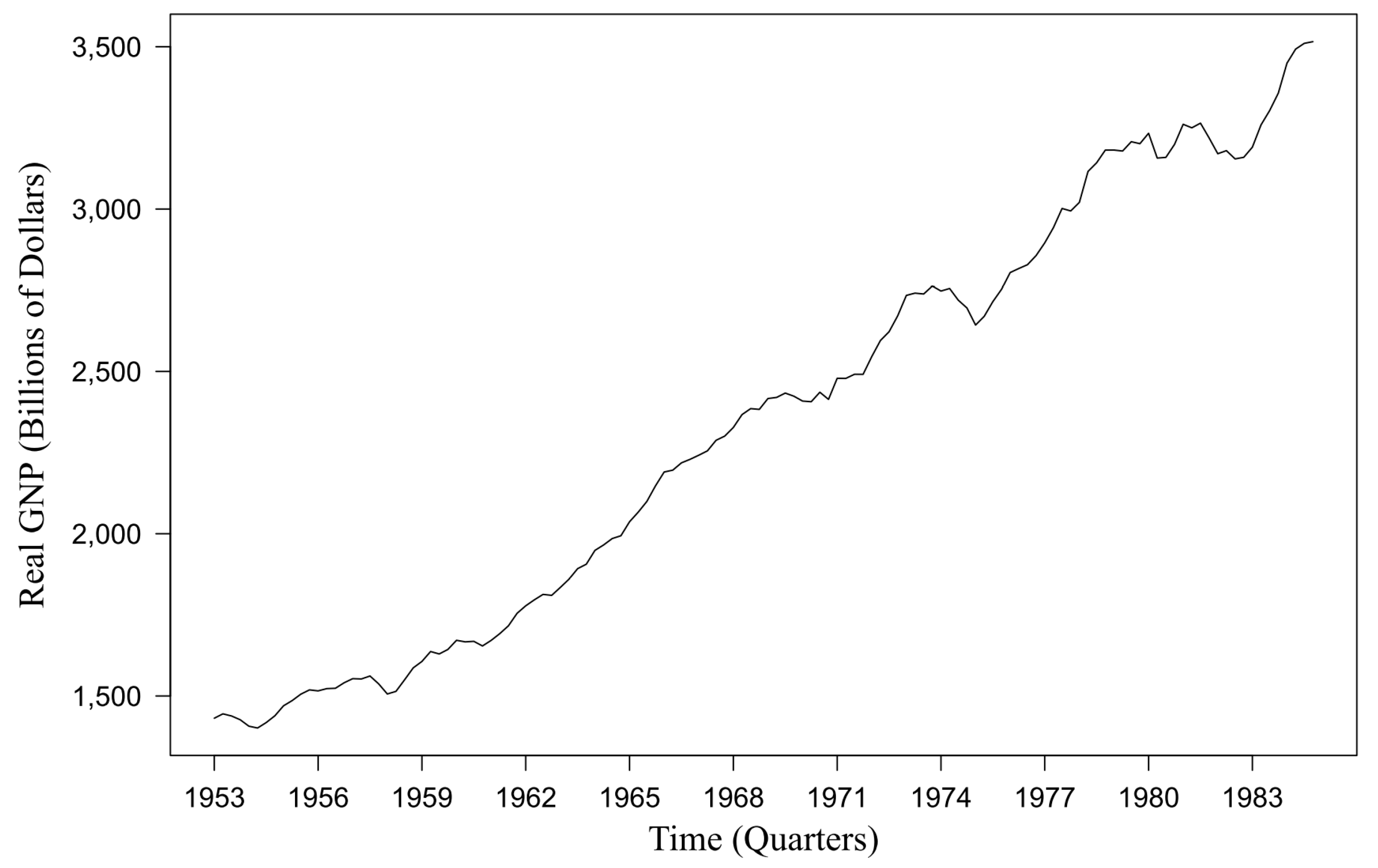
We utilized historical data from the MSAR model by Hamilton [3], directly comparing its performance with our MSAR-TVP model using the same U.S. real GNP dataset. These data were expressed in billions of chained 1982 dollars and were sourced from the Business Conditions Digest of February 1986, specifically from series 50, page 102. Prior to transitioning to a detailed exploration of the dataset, it is crucial to first understand the fundamental characteristics of the data used in our study. Figure 1 displays the time series plot for the real GNP data (denoted as Z t ) from Q3 1952 to Q4 1984.
The trend depicted in Figure 1 illustrates the cyclical changes in the U.S. economy, characterized by alternating regimes of expansion and recession. The observed variability reflects how the economy adjusts to various internal and external influences. Fluctuations in the data indicate the potential for structural changes during the observation period.
The data in Table 2 indicate that the highest value of real GNP data is 3516, while the lowest is 1378, with an average of 2332 over the 130 quarters observed. A standard deviation of 654.1368 marks the volatility of the data. A skewness close to zero, at 0.0991, suggests that the distribution of values is relatively symmetric around the mean. Furthermore, a kurtosis value of 1.6679, which is less than 3, confirms that the distribution is platykurtic, characterized by shorter tails and fewer extreme values compared to a normal distribution.

3.1.2. The MSAR-TVP Model

The MSAR-TVP model is well-suited to analyzing data that exhibit structural changes, as evidenced by the statistical significance detected through the Chow test [45] on real GNP data ( Z t ) . A very small p -value of less than 2.2 × 10 16 strongly rejects the null hypothesis and confirms significant structural changes. Consequently, the MSAR-TVP model, which adopts a two-regime approach each following an AR(1) process, was implemented.
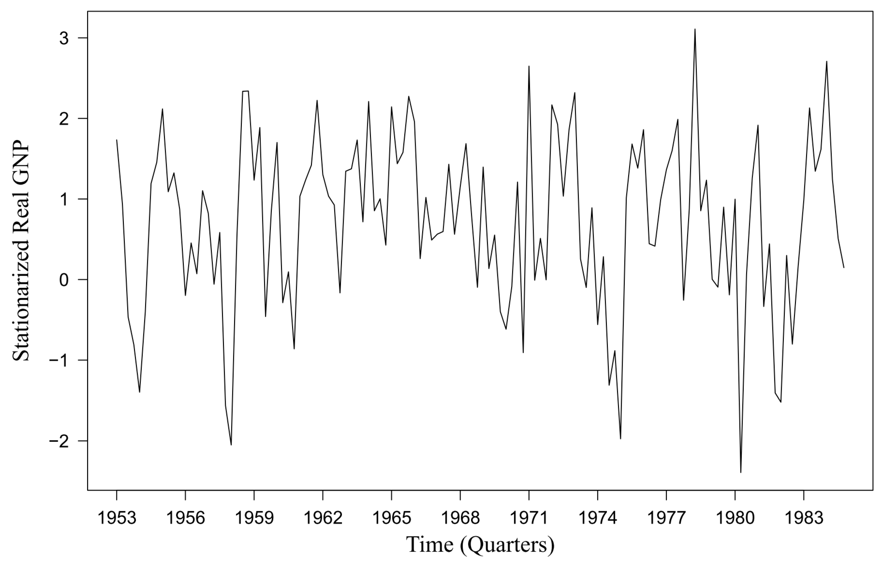
The test for variance stationarity using the Box–Cox transformation [46] resulted in a λ = 0 , suggesting that a logarithmic transformation, Z t * = ln ( Z t ) , is necessary to achieve variance stationarity. Meanwhile, the augmented Dickey–Fuller (ADF) test [35] for mean stationarity on Z t * yielded a p -value of 0.0899, indicating that the time series is still non-stationary in mean. Therefore, a differencing process [47] was employed to address this mean non-stationarity. Finally, model analysis was performed on 100 times the log-difference in quarterly real GNP, or Y t = 100 × Δ ln ( Z t ) . The trend depicted in Figure 2 illustrates the cyclical changes in the U.S. economy, characterized by alternating regimes of expansion and recession.
The MSAR-TVP model is implemented with two regimes: Regime 1, representing an expansion state, and Regime 2, representing a recession state. Each regime is assumed to follow an AR(1) process, allowing the real GNP data to be modeled in an MS(2)-AR(1)-TVP framework. Model estimation is carried out using the MLE approach, with optimization performed through the Nelder–Mead algorithm and dynamic parameter adjustments facilitated by the Kim filter. The estimated model delineates two states, each characterized by specific equations:
For S t = 1 :
Y ^ t = μ ^ 1 * + Y t 1 β ^ t , 1 , 1 ,
β ^ t , 1 , 1 = δ ^ 1 , 1 * + 0.9712 β t 1 , 1 , 1 ,
For S t = 2 :
Y ^ t = μ ^ 2 * + Y t 1 β ^ t , 1 , 2 ,
β ^ t , 1 , 2 = δ ^ 1 , 2 * + 0.2551 β t 1 , 1 , 2 ,
The transition probability matrix obtained is:
P = 0.9125 0.0875 0.1254 0.8746 .
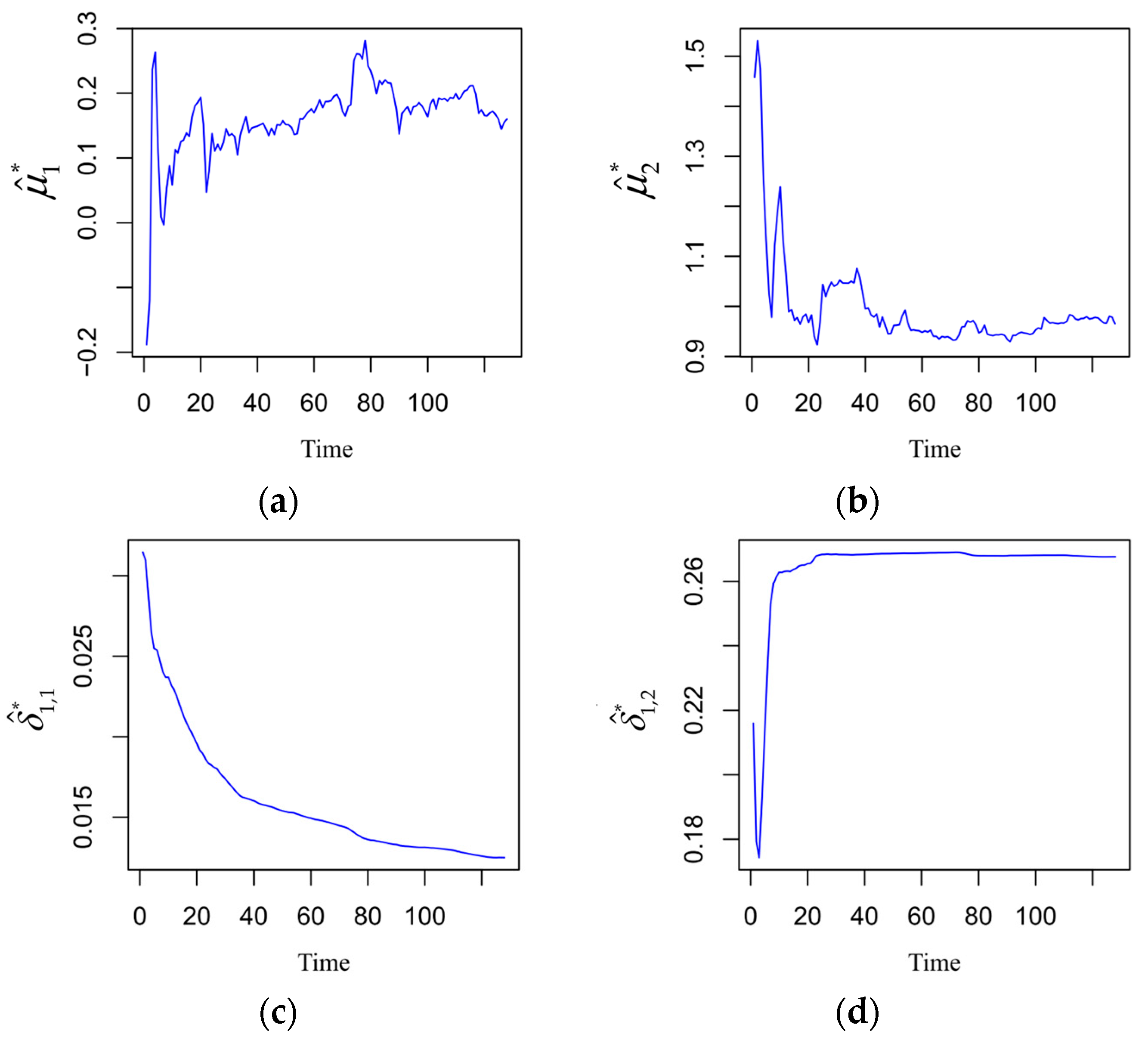
The time-varying parameter estimates for β ^ t , 1 , S t are illustrated in Figure 3, while estimates for other parameters across different time points, such as μ ^ S t * and δ ^ 1 , S t * , are displayed in Figure 4. The estimation results indicate that the model has converged, achieving a maximum log-likelihood value of 184.6007 .
The transition probability matrix in Equation (50) illustrates the probabilities of transitioning between two regimes in the MSAR-TVP model. The probability of switching from Regime 1 to Regime 2 is 0.0875, indicating an 8.75% chance of transition. Conversely, the probability of moving from Regime 2 to Regime 1 is 0.1254, indicating a 12.54% chance of transition. The relatively high probabilities on the diagonal (0.9125 for staying in Regime 1 and 0.8746 for staying in Regime 2) suggest a greater likelihood of remaining in the current regime rather than switching, indicating stability within each regime.
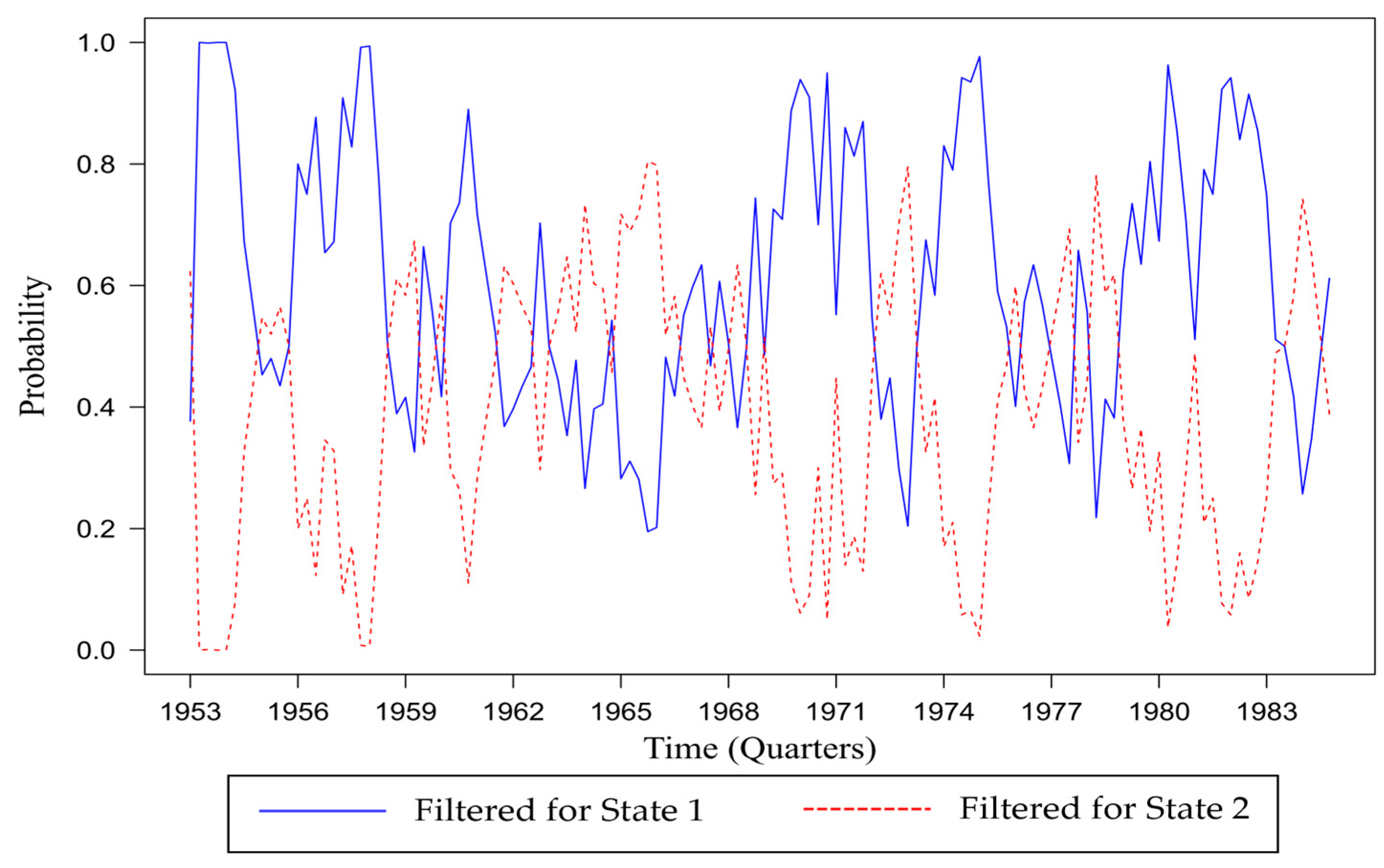
Estimation insights into the filtered probabilities are illustrated in Figure 5, which shows the conditional probabilities of each regime based on available data. Specifically, this is represented by P ( S t = 1 Y t ) for Regime 1 (Filtered for State 1) and P ( S t = 2 Y t ) for Regime 2 (Filtered for State 2), where Y t is the observed information. In Figure 5, Filtered for State 1 is shown as a solid blue line and Filtered for State 2 as a dashed red line. These distinct line styles and colors help distinguish the two regimes, simplifying the visual analysis of changes in regime dynamics.
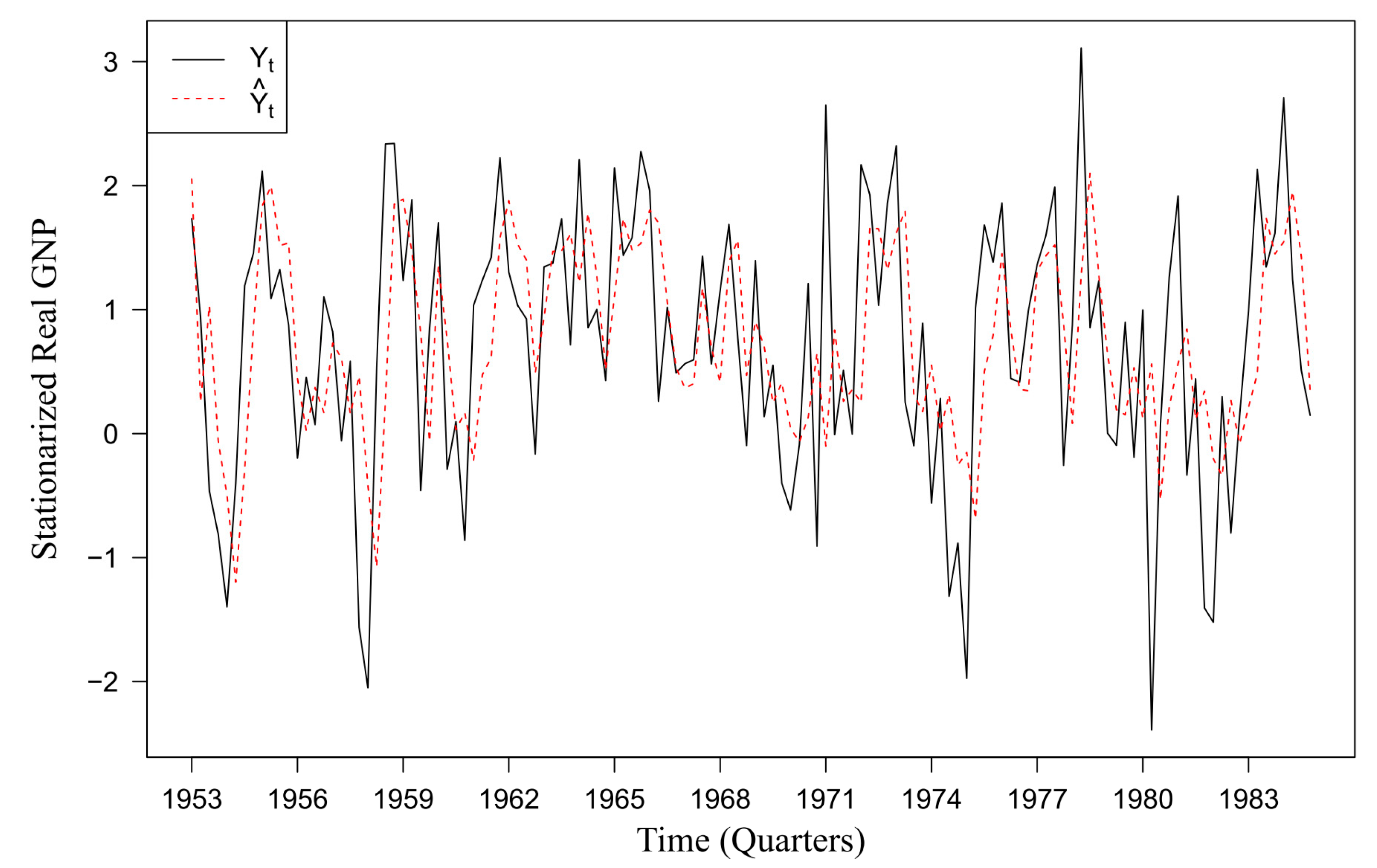
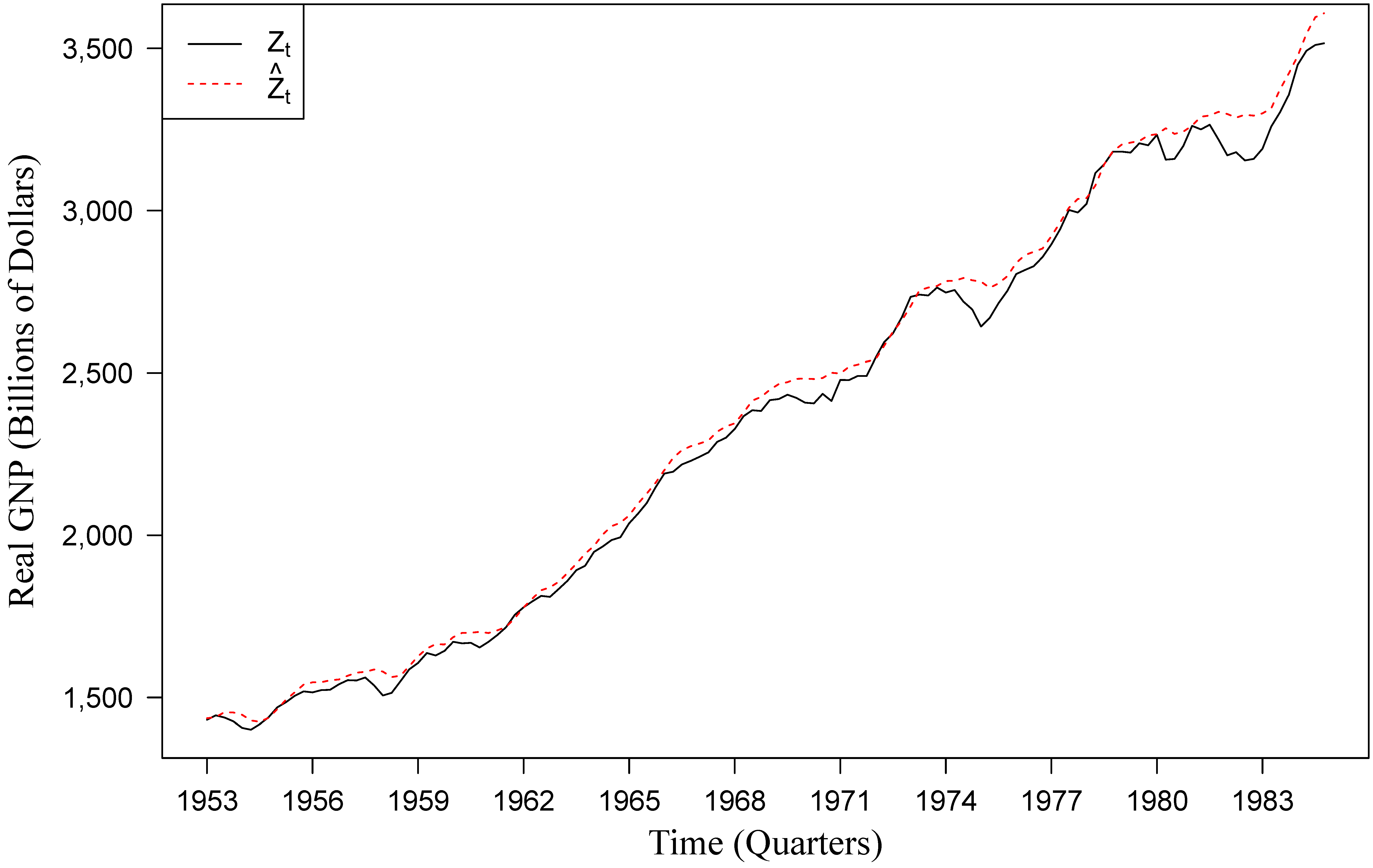
Figure 6 presents a comparison between the stationarized real GNP data, Y t , and its predictions, Y ^ t , by the MSAR-TVP model, highlighting the model’s accuracy in capturing the dynamics of the data. Figure 7 compares the original scale’s actual values, Z t , with its predictions, Z ^ t , demonstrating the MSAR-TVP model’s precision.

3.1.3. Comparison of MSAR-TVP and MSAR Models

We conducted a comparison between the MSAR-TVP model and the MSAR model, using U.S. real GNP data. Both the MSAR-TVP and MSAR models were constructed under the assumption that the model follows an AR(1) process with two regimes. The comparison was performed for both in-sample and out-of-sample data. The in-sample data use real GNP from Q3 1952 to Q4 1984, while the out-of-sample data cover Q1 1985 to Q4 1986. The out-of-sample data were obtained from the Business Conditions Digest of March 1990, specifically from series 50, page 80.
Table 3 presents the in-sample performance of the MSAR-TVP and MSAR models. The MAPE and MAE were used as the evaluation metrics. The results shown in Table 3 indicate that our proposed model, MSAR-TVP, outperforms the MSAR model in analyzing real GNP data. This is evidenced by the achievement of the lowest MAPE and MAE values. Specifically, the MSAR-TVP model achieved a MAPE of 1.53% and an MAE of 36.58, significantly lower than the MSAR model’s MAPE of 3.30% and MAE of 62.49. The improved performance of the MSAR-TVP model suggests its superior capability in capturing the underlying patterns and structural changes within the in-sample data.
Table 4 presents the out-of-sample performance of the MSAR-TVP and MSAR models. The MAPE and MAE were evaluated quarterly from Q1 1985 to Q4 1986. The out-of-sample results in Table 4 consistently show that the MSAR-TVP model outperforms the MSAR model across all quarters. The MSAR-TVP model yields lower MAPE and MAE values in each period, indicating its robustness in predicting out-of-sample data. For instance, in Q1 1985, the MSAR-TVP model achieved a MAPE of 1.93% compared to the MSAR model’s 2.03%. This trend continues throughout the out-of-sample period, with the MSAR-TVP model maintaining lower error rates. Additionally, the forecast for the next eight periods indicates that the economy remains in State 1 (expansion), reflecting the model’s ability to capture and predict economic trends accurately. A possible explanation for the success of the MSAR-TVP model may be due to its ability to dynamically identify structural changes in each regime, effectively capturing stochastic changes in the data that are difficult to explain by linear or non-linear models with fixed parameters.
Diagnostic tests displayed in Table 5 support the assumption that residuals in both regimes of the MSAR-TVP and MSAR models adhere to a normal distribution and exhibit white noise properties. The p -values from the Kolmogorov–Smirnov (KS) test [48] and the Durbin–Watson (DW) test [49,50] are all greater than the significance level α of 0.05. These results indicate that the residuals from the MSAR-TVP and MSAR models meet the basic assumptions necessary for valid statistical analysis.
In conclusion, the MSAR-TVP model demonstrates superior performance in both in-sample and out-of-sample analyses of U.S. real GNP data, making it a valuable tool for capturing dynamic structural changes in economic time series data.

3.2. Forecasting U.S. Real GNP Using the MSAR-TVP Model (1947–2024)

We extended the dataset of U.S. real GNP quarterly data from Q1 1947 to Q1 2024 (denoted as W t ), which is publicly available from the Federal Reserve Economic Data (FRED). This dataset represents billions of chained 2017 dollars, quarterly and at a seasonally adjusted annual rate, comprising 309 observations. The analysis follows the steps outlined in the previous sections, with this section focusing on forecasting. The modeling was performed on the stationary data, V t = 100 × Δ ln ( W t ) .
The MSAR-TVP model was implemented for two regimes: Regime 1 represents the expansion state and Regime 2 represents the recession state, with each regime following an AR(1) process. Based on the parameter estimates, the mathematical formulation of the MS(2)-AR(1)-TVP model is as follows:
For S t = 1 :
V ^ t = μ ^ 1 * + V t 1 β ^ t , 1 , 1 ,
β ^ t , 1 , 1 = δ ^ 1 , 1 * + 0.2242 β t 1 , 1 , 1 ,
For S t = 2 :
V ^ t = μ ^ 2 * + V t 1 β ^ t , 1 , 2 ,
β ^ t , 1 , 2 = δ ^ 1 , 2 * + 0.0851 β t 1 , 1 , 2 ,
The transition probability matrix obtained is:
P = 0.9931 0.0069 0.0240 0.9760 .
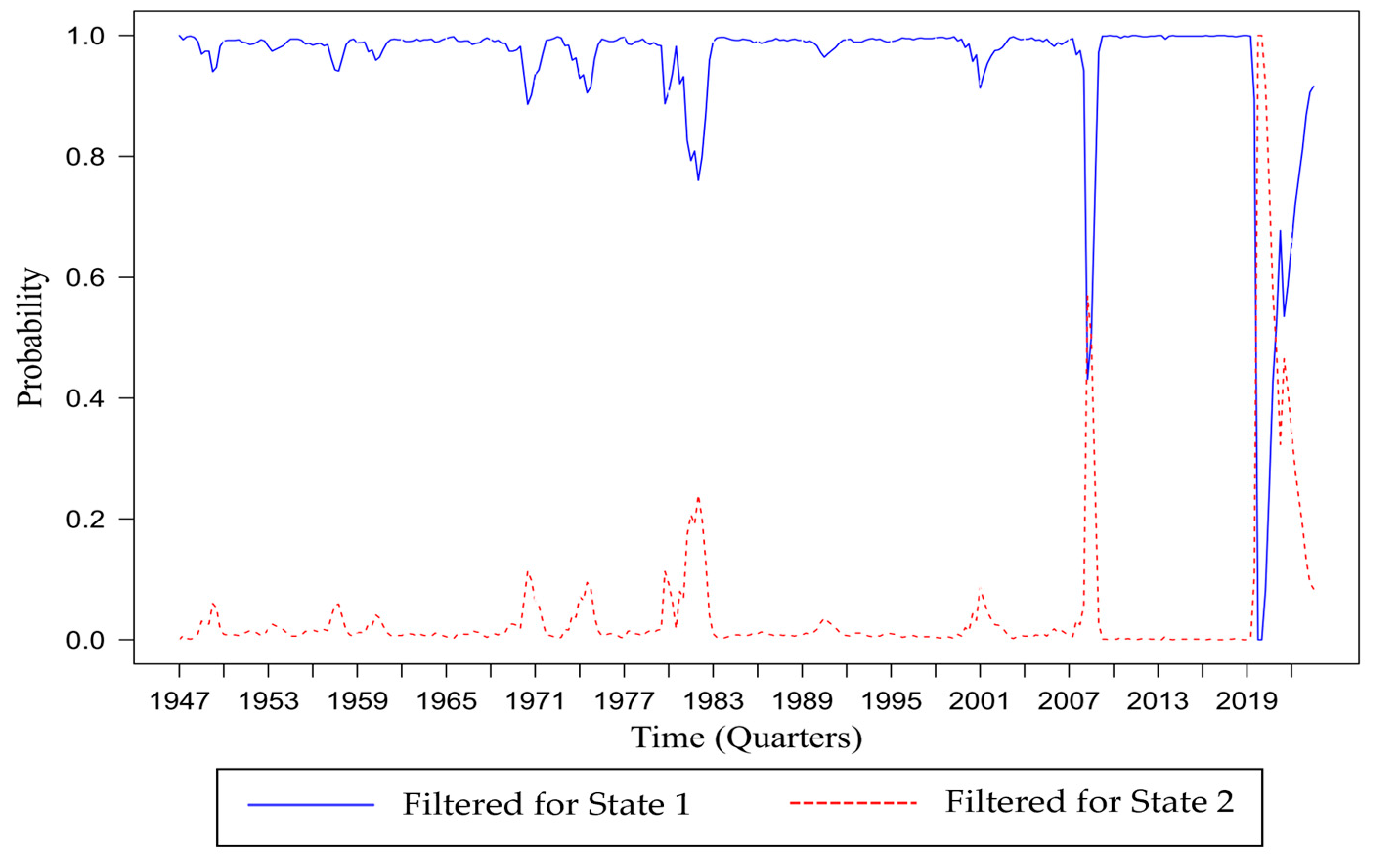
Figure 8 shows estimation insights into the filtered probabilities, which represent the conditional probabilities of each regime based on available data. The filtered probability plot for the extended real GNP data from 1947 to 2024 highlights significant economic events. Notably, during the 2008 global financial crisis, there was a marked increase in the probability of being in a recession state (State 2), with a recession probability of 0.569. Similarly, the COVID-19 pandemic in 2020–2021 caused a dramatic economic downturn, with the probability peaking at 1. These periods of recession contrast with the generally high probability of economic expansion (State 1) observed during other times, reflecting periods of sustained economic growth. The model’s ability to accurately capture these fluctuations underscores its effectiveness in identifying and analyzing major economic shifts over time.
Table 6 presents the analysis results for the U.S. real GNP data from Q1 1947 to Q1 2024. The MSAR-TVP model yielded a MAPE of 5.24% and an MAE of 709.28. The MAPE value falls within the criteria for a highly accurate forecast, indicating that the model’s predictions are close to the actual values on a percentage basis. The MAE value of 709.28 represents the average absolute difference between the predicted and actual real GNP values, which provides a measure of the magnitude of the forecast errors in real terms. These results are supported by full compliance with the assumptions of normality and white noise of residuals, ensuring the validity and reliability of the model.
According to the KS test for residuals, the MSAR-TVP model satisfies the normality assumption for both regimes at the significance level of α = 0.05 , as the p -values for both regimes are greater than 0.05. For the DW test, both regimes satisfy the white noise assumption since the p -values are greater than 0.05. This indicates that the model is validated and proven to be reliable.
Table 7 presents the average run length (ARL) calculation in the extended dataset, revealing key insights into the duration of economic regimes. For State 1 (expansion), the ARL is 99.67 quarters, significantly longer than for State 2 (recession), which has an ARL of 2.33 quarters. This suggests that expansion periods tend to last much longer than recession periods. The maximum run length for expansions is 244 quarters, with a minimum of 11 quarters, while recessions have a maximum run length of 5 quarters and a minimum of 1 quarter. These findings are crucial for economic planning and business strategy, indicating that economic growth phases are typically more prolonged, but businesses must be prepared for shorter, albeit potentially more impactful, recession periods. The number of runs observed, with three expansion cycles and three recession cycles, highlights that recessions, despite being shorter, occur as frequently as expansions and must be anticipated in economic planning.
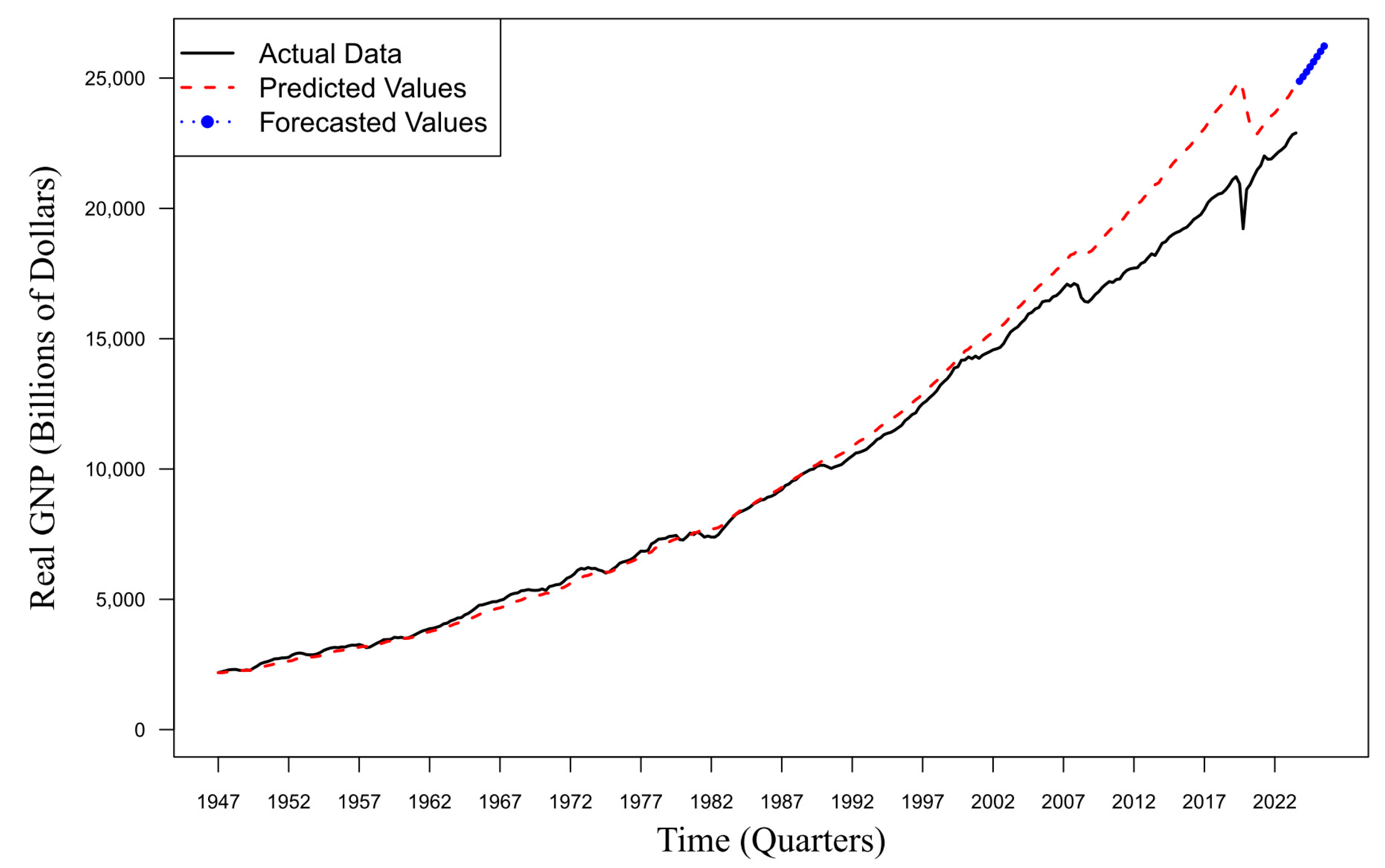
Figure 9 presents the forecasted values of the U.S. real GNP from Q1 1947 to Q1 2024, alongside the actual observed values, and the two-year ahead forecast from Q2 2024 to Q1 2026. The black line represents the actual data from Q1 1947 to Q1 2024, while the red dashed line represents the predicted values for the same period. Additionally, the blue dotted line with points represents the forecasted values for the periods from Q2 2024 to Q1 2026. Utilizing the MSAR-TVP model with two regimes, representing expansion and recession phases, and an AR order of 1, the two-year ahead forecast indicates a significant increase, predominantly in the expansion phase. From Figure 9, it is evident that the in-sample forecasted values closely follow the observed values throughout the entire period, indicating a good fit for the model. The high degree of alignment between the two lines suggests that the model effectively captures the underlying trend and structural changes in the U.S. real GNP data over time.
This visual observation is further supported by the previously discussed MAPE of 5.24%, which signifies the model’s reliability and accuracy in predicting the U.S. real GNP. Overall, the close correspondence between the observed and forecasted values in Figure 9, combined with the low MAPE, confirms the model’s strong performance in capturing the dynamics of the U.S. real GNP over the analyzed period. The additional out-of-sample forecasted values further indicate the model’s potential for reliable future predictions.

4. Discussion and Future Research Directions

This study offers new insights into time series modeling and forecasting for data undergoing structural changes, such as U.S. real GNP, using the MSAR-TVP model. This model aims to handle nonlinear data that experience structural changes, addressing the non-stationarity inherent in economic data. Compared to the MSAR model, the MSAR-TVP model shows superior predictive accuracy with lower MAPE and MAE values. The model is effectively used for forward forecasting.
The time-varying parameters in the MSAR-TVP model allow it to adapt to data changes over time, providing more accurate estimates. The model’s flexibility and robustness make it suitable for short-term forecasting, as it can maintain high accuracy despite the increasing complexity of economic data. The outcomes demonstrate the MSAR-TVP model’s potential as a valuable tool for economic analysis and policy-making.
However, given the increasing complexity of economic data, there are several limitations to the current model that warrant consideration for future enhancements. The model currently assumes that each regime follows an AR(1) process, which simplifies computation but may limit its ability to capture more complex economic dynamics. Future research should explore increasing the AR order to more than one. Expanding the number of regimes beyond two could allow the model to capture a broader range of economic states and transitions, thus better reflecting the complexities of economic data. Additionally, incorporating residual errors that follow a non-Gaussian distribution [51,52,53] could improve the model’s robustness, especially in the presence of outliers or heavy-tailed distributions.
Moreover, modifying the model by using pairwise Markov models (PMMs) instead of classical hidden Markov models (HMMs), which share some similarities with state-space models, is also compelling. PMMs can provide a more general framework and improve the efficiency of the proposed model [54,55,56,57]. Furthermore, the development of more advanced estimation methods, such as adopting a Bayesian approach to parameter estimation, could enhance the model’s flexibility and reliability, particularly for complex datasets. These enhancements could potentially improve the model’s adaptability and accuracy in forecasting complex economic dynamics.

5. Conclusions

In this study, we proposed the MSAR-TVP model, an adaptation of the MSAR model that incorporates time-varying parameters to address the challenges of nonlinear time series undergoing structural changes. This model combines the effective regime identification capability of the MSAR with the flexibility of time-varying parameters to enhance prediction accuracy. The MSAR-TVP model was evaluated using U.S. real GNP data from Q3 1952 to Q4 1984 as in-sample data and from Q1 1985 to Q4 1986 as out-of-sample data, comparing its performance to the conventional MSAR model. Additionally, the model was applied to an extended dataset from Q1 1947 to Q1 2024 to demonstrate its forecasting effectiveness.
The parameter estimation method for the MSAR-TVP model employs MLE enriched with the Kim filter, a fusion of the Kalman filter, Hamilton filter, and Kim collapsing. This approach, optimized through the Nelder–Mead algorithm, significantly enhances the accuracy and efficiency of data processing, allowing the model to dynamically respond to changes in the data while adhering to the assumptions of normal distribution and white noise residuals.
Overall, the findings indicate that the MSAR-TVP model, utilizing the developed parameter estimation method, provides a more precise and reliable framework for capturing economic fluctuations, particularly in identifying structural changes in the applied data cases. The model consistently outperforms the MSAR model in forecasting error metrics, both in-sample and out-of-sample, achieving lower MAPE and MAE values. The extended dataset from Q1 1947 to Q1 2024 further validated the model’s forecasting effectiveness, demonstrating its robustness and accuracy in predicting future economic trends.
The outcomes of this study demonstrate the MSAR-TVP model’s improved accuracy over the MSAR model. This advancement aids in better predicting economic fluctuations, supporting informed economic policy decisions and data-driven planning. The model’s performance underscores its potential utility in various forecasting applications, contributing to the development of econometric methods. While the model shows significant promise, it is important to consider its limitations and the potential for further refinement.
Author Contributions

Conceptualization, S.I.; methodology, S.I. and N.I.; software, S.I.; validation, S.I., N.I. and I.; formal analysis, S.I. and N.I.; investigation, S.I.; resources, S.I.; writing—original draft preparation, S.I.; writing—review and editing, N.I. and I.; visualization, S.I.; supervision, N.I. and I.; project administration, S.I.; funding acquisition, S.I. All authors have read and agreed to the published version of the manuscript.

Funding

This research was funded by the Center for Higher Education Funding (Balai Pembiayaan Pendidikan Tinggi, BPPT) under the Ministry of Education, Culture, Research, and Technology (Kemendikbudristek) and the Indonesia Endowment Fund for Education (Lembaga Pengelola Dana Pendidikan, LPDP) under the Ministry of Finance of the Republic of Indonesia.

Data Availability Statement

The data for real GNP used in this research were sourced from the Business Conditions Digest of February 1986 and March 1990. Access to the data is available at: https://fraser.stlouisfed.org/title/business-conditions-digest-43?browse=1980s#7474 (accessed on 31 May 2023). The extended dataset, covering 1 January 1947 to 1 January 2024, is publicly available from the Federal Reserve Economic Data (FRED), supplied by the St. Louis Fed, at https://fred.stlouisfed.org/series/GNPC96 (accessed on 31 March 2024).

Acknowledgments

The first author thanks BPPT and LPDP Indonesia for the financial support under the Doctoral Program Scholarship. The authors are grateful to the Department of Statistics, Faculty of Science and Data Analytics, Institut Teknologi Sepuluh Nopember (ITS), for their invaluable support and collaboration. Special thanks are also due to colleagues for their invaluable inputs during discussions throughout the research.

Conflicts of Interest

The authors declare no conflicts of interest.

References

  1. Meyler, A.; Kenny, G.; Quinn, T. Forecasting Irish Inflation Using ARIMA Models. Econ. Anal. Res. Publ. Dep. Cent. Bank Irel. 1998, 1998, 1–48. [Google Scholar]
  2. Tzagkarakis, G.; Dionysopoulos, T.; Achim, A. Recurrence Quantification Analysis of Denoised Index Returns via Alpha-Stable Modeling of Wavelet Coefficients: Detecting Switching Volatility Regimes. Stud. Nonlinear Dyn. Econom. 2016, 20, 75–96. [Google Scholar] [CrossRef]
  3. Hamilton, J.D. A New Approach to the Economic Analysis of Nonstationary Time Series and the Business Cycle. Econometrica 1989, 57, 357–384. [Google Scholar] [CrossRef]
  4. Box, G.E.P.; Jenkins, G.M. Time Series Analysis: Forecasting and Control; Holden-Day: Oakland, CA, USA, 1976. [Google Scholar]
  5. Adebiyi, A.A.; Adewumi, A.O.; Ayo, K.A. Stock Price Prediction Using the ARIMA Model. In Proceedings of the 2014 UKSim-AMSS 16th International Conference on Computer Modelling and Simulation, Cambridge, UK, 26–28 March 2014; pp. 106–112. [Google Scholar]
  6. Pok-sang, L. The Hamilton Model with a General Autoregressive Component: Estimation and Comparison with Other Models of Economic Time Series. J. Monet. Econ. 1990, 26, 409–432. [Google Scholar] [CrossRef]
  7. Kim, C.J.; Nelson, C.R. Has the U.S. Economy Become More Stable? A Bayesian Approach Based on a Markov-Switching Model of the Business Cycle. Rev. Econ. Stat. 1999, 81, 608–616. [Google Scholar] [CrossRef]
  8. Adejumo, O.A.; Albert, S.; Asemota, O.J. Markov Regime-Switching Autoregressive Model of Stock Market Returns in Nigeria. CBN J. Appl. Stat. 2020, 11, 65–83. [Google Scholar] [CrossRef]
  9. Prihartanti, W.; Rasyid, D.A.; Iriawan, N. Daily Stock Price Regime Model Detection Using Markov Switching Model. Mat. MJIAM 2020, 36, 127–140. [Google Scholar] [CrossRef]
  10. Stillwagon, J.; Sullivan, P. Markov Switching in Exchange Rate Models: Will More Regimes Help? Empir. Econ. 2020, 59, 413–436. [Google Scholar] [CrossRef]
  11. Lukianenko, I.; Nasachenko, M. Inflation Expectations Modeling: The Application of Markov Switching Autoregression. Sci. Pap. Nauk. Econ. 2020, 5, 82–88. [Google Scholar] [CrossRef]
  12. Hamilton, J.D.; Susmel, R. Autoregressive Conditional Heteroskedasticity and Changes in Regime. J. Econom. 1994, 64, 307–333. [Google Scholar] [CrossRef]
  13. Gray, S.F. Modeling the Conditional Distribution of Interest Rates as a Regime-Switching Process. J. Financ. Econ. 1996, 42, 27–62. [Google Scholar] [CrossRef]
  14. Bazzi, M.; Blasques, F.; Koopman, S.J.; Lucas, A. Time-Varying Transition Probabilities for Markov Regime Switching Models. J. Time Ser. Anal. 2016, 38, 458–478. [Google Scholar] [CrossRef]
  15. Maneejuk, P.; Yamaka, W.; Sriboonchitta, S. A Markov-Switching Model with Mixture Distribution Regimes. In International Symposium on Integrated Uncertainty in Knowledge Modelling; Springer: Cham, Switzerland, 2018; pp. 312–323. [Google Scholar]
  16. Tanizaki, H. The Time-Varying Parameter Model Revisited. Kobe Univ. Econ. Rev. 1999, 45, 41–57. [Google Scholar]
  17. Fornaciari, M.; Grillenzoni, C. Evaluation of On-line Trading Systems: Markov-Switching vs Time-Varying Parameter Models. Decis. Support Syst. 2017, 93, 51–61. [Google Scholar] [CrossRef]
  18. Kalman, R.E. A New Approach to Linear Filtering and Prediction Problems. J. Basic Eng. 1960, 82, 35–45. [Google Scholar] [CrossRef]
  19. Rosenberg, B. A Survey of Stochastic Parameter Regression. Ann. Econ. Soc. Meas. 1973, 2, 380–396. [Google Scholar]
  20. Anderson, B.D.O.; Moore, J.B. Optimal Filtering; Prentice-Hall, Inc.: Upper Saddle River, NJ, USA, 1979. [Google Scholar]
  21. Hamilton, J.D. State-Space Models. In Handbook of Econometrics; Engle, R.F., McFadden, D.L., Eds.; Chapter 50; Elsevier B.V.: Amsterdam, The Netherlands, 1994; Volume 4, pp. 3041–3080. [Google Scholar]
  22. Kim, C.J. Dynamic Linear Models with Markov-Switching. J. Econom. 1994, 60, 1–22. [Google Scholar] [CrossRef]
  23. Kim, C.J.; Nelson, C.R. State-Space Models with Regime Switching: Classical and Gibbs-Sampling Approaches with Applications; The MIT Press: Cambridge, MA, USA, 2000. [Google Scholar]
  24. Kim, C. Unobserved-Component Time Series Models with Markov-Switching in Heteroscedasticity: Changes in Regime and the Link between Inflation Rates and Inflation Uncertainty. J. Bus. Econ. Stat. 1993, 11, 341–349. [Google Scholar] [CrossRef]
  25. Gangloff, H.; Morales, K.; Petetin, Y. Deep Parameterizations of Pairwise and Triplet Markov Models for Unsupervised Classification of Sequential Data. Comput. Stat. Data Anal. 2023, 180, 107663. [Google Scholar] [CrossRef]
  26. Ben Abbes, A.; Farah, M.; Farah, I.R.; Barra, V. A Non-Stationary NDVI Time Series Modelling Using Triplet Markov Chain. Int. J. Inf. Decis. Sci. 2019, 11, 163–179. [Google Scholar] [CrossRef]
  27. Zheng, F.; Derrode, S.; Pieczynski, W. Semi-Supervised Optimal Recursive Filtering and Smoothing in Non-Gaussian Markov Switching Models. Signal Process. 2020, 171, 107511. [Google Scholar] [CrossRef]
  28. Chen, S.; Jiang, X. Modeling Repayment Behavior of Consumer Loan in Portfolio across Business Cycle: A Triplet Markov Model Approach. Complexity 2020, 2020, 5458941. [Google Scholar] [CrossRef]
  29. Degras, D.; Ting, C.M.; Ombao, H. Markov-Switching State-Space Models with Applications to Neuroimaging. Comput. Stat. Data Anal. 2022, 174, 107525. [Google Scholar] [CrossRef]
  30. Conn, A.R.; Scheinberg, K.; Vicente, L.N. Introduction to Derivative-Free Optimization; Society for Industrial and Applied Mathematics: Philadelphia, PA, USA, 2009. [Google Scholar]
  31. Nelder, J.A.; Mead, R. A Simplex Method for Function Minimization. Comput. J. 1965, 7, 308–313. [Google Scholar] [CrossRef]
  32. Ozaki, Y.; Yano, M.; Onishi, M. Effective Hyperparameter Optimization Using Nelder-Mead Method in Deep Learning. IPSJ Trans. Comput. Vis. Appl. 2017, 9, 20. [Google Scholar] [CrossRef]
  33. Hamilton, J.D. Time Series Analysis; Princeton University Press: Princeton, NJ, USA, 1994. [Google Scholar]
  34. Harvey, A.C. Forecasting, Structural Time Series Models and the Kalman Filter; Cambridge University Press: New York, NY, USA, 1989. [Google Scholar]
  35. Gujarati, D.N.; Porter, D.C. Basic Econometrics, 5th ed.; McGraw-Hill: New York, NY, USA, 2012. [Google Scholar]
  36. Casas, I.; Fernandez-Casal, R. tvReg: Time-Varying Coefficient Linear Regression for Single and Multi-Equations in R. SSRN Electron. J. 2019, 1–43. [Google Scholar] [CrossRef]
  37. Rajan, J.J.; Rayner, P.J.W.; Godsill, S.J. Bayesian Approach to Parameter Estimation and Interpolation of Time-Varying Autoregressive Processes Using the Gibbs Sampler. IEE Proc. Vis. Image Signal Process. 1997, 144, 249–255. [Google Scholar] [CrossRef]
  38. Rajan, J.J.; Rayner, P.J.W. Parameter Estimation of Time-Varying Autoregressive Models Using the Gibbs Sampler. Electron. Lett. 1995, 31, 1035–1036. [Google Scholar] [CrossRef]
  39. Hamilton, J.D. Specification Testing in Markov-Switching Time-Series Models. J. Econom. 1996, 70, 127–157. [Google Scholar] [CrossRef]
  40. Doornik, J.A. A Markov-Switching Model with Component Structure for US GNP. Econ. Lett. 2013, 118, 265–268. [Google Scholar] [CrossRef]
  41. R Core Team and Contributors Worldwide. The R Stats Package, Version 4.3.1. Available online: https://www.rdocumentation.org/packages/stats/versions/3.6.2/topics/optim (accessed on 25 June 2023).
  42. Vega, R.; Flores, L.; Greiner, R. SIMLR: Machine Learning inside the SIR Model for COVID-19 Forecasting. Forecasting 2022, 4, 72–94. [Google Scholar] [CrossRef]
  43. Montaño Moreno, J.J.; Palmer Pol, A.; Sesé Abad, A.; Cajal Blasco, B. Using the R-MAPE Index as a Resistant Measure of Forecast Accuracy. Psicothema 2013, 25, 500–506. [Google Scholar] [CrossRef] [PubMed]
  44. Lewis, C.D. Industrial and Business Forecasting Methods: A Practical Guide to Exponential Smoothing and Curve Fitting; Heinemann: Penang, Malaysia, 1982. [Google Scholar]
  45. Chow, G.C. Tests of Equality Between Sets of Coefficients in Two Linear Regressions. Econometrica 1960, 28, 591–605. [Google Scholar] [CrossRef]
  46. Box, G.E.P.; Cox, D.R. An Analysis of Transformations. J. R. Stat. Soc. Ser. B 1964, 26, 211–252. [Google Scholar] [CrossRef]
  47. Wei, W.W.S. Time Series Analysis: Univariate and Multivariate Methods; Pearson Education, Inc.: San Francisco, CA, USA, 2006. [Google Scholar]
  48. Daniel, W.W. Applied Nonparametric Statistics, 2nd ed.; PWS-Kent: Boston, MA, USA, 2000. [Google Scholar]
  49. Durbin, J.; Watson, G.S. Testing for Serial Correlation in Least Squares Regression, I. Biometrika 1950, 37, 409–428. [Google Scholar] [CrossRef]
  50. Durbin, J.; Watson, G.S. Testing for Serial Correlation in Least Squares Regression, II. Biometrika 1951, 38, 159–177. [Google Scholar] [CrossRef] [PubMed]
  51. Choir, A.S.; Iriawan, N.; Mutmainah, S.S.K. Neojags: Neo-Normal Distributions Family for Markov Chain Monte Carlo (MCMC) Models in JAGS (Version 0.1.4) [R Package]. CRAN. Available online: https://cran.r-project.org/web/packages/neojags/index.html (accessed on 3 July 2024).
  52. Choir, A.S.; Iriawan, N.; Suprih Ulama, B.S.; Dokhi, M. MSEPBurr Distribution: Properties and Parameter Estimation. Pakistan J. Stat. Oper. Res. 2019, 15, 179–193. [Google Scholar] [CrossRef]
  53. Iriawan, N. Computationally Intensive Approaches to Inference in Neo-Normal Linear Models; Curtin University of Technology: Bentley, UK, 2000. [Google Scholar]
  54. Petetin, Y.; Desbouvries, F. Bayesian Multi-Object Filtering for Pairwise Markov Chains. IEEE Trans. Signal Process. 2013, 61, 4481–4490. [Google Scholar] [CrossRef]
  55. Kulikova, M.V.; Tsyganova, J.V.; Kulikov, G.Y. UD-Based Pairwise and MIMO Kalman-Like Filtering for Estimation of Econometric Model Structures. IEEE Trans. Automat. Contr. 2020, 65, 4472–4479. [Google Scholar] [CrossRef]
  56. Mahler, R. The Pairwise-Markov Bernoulli Filter. IEEE Access 2020, 8, 168229–168245. [Google Scholar] [CrossRef]
  57. Nemesin, V.; Derrode, S. Robust Partial-Learning in Linear Gaussian Systems. IEEE Trans. Automat. Contr. 2015, 60, 2518–2523. [Google Scholar] [CrossRef]
Figure 1. Time series plot of U.S. real GNP (1952–1984).
Forecasting 06 00031 g001
Figure 2. Time series plot of the stationarized real GNP ( Y t ) (1952–1984).
Forecasting 06 00031 g002
Figure 3. Time-varying parameters of the MSAR-TVP: (a) β ^ t , 1 , 1 , (b) β ^ t , 1 , 2 .
Forecasting 06 00031 g003
Figure 4. Parameter values across different time points: (a) μ ^ 1 * , (b) μ ^ 2 * , (c) δ ^ 1 , 1 * , (d) δ ^ 1 , 2 * .
Forecasting 06 00031 g004
Figure 5. Filtered probabilities for real GNP: MSAR-TVP Model (1952–1984).
Forecasting 06 00031 g005
Figure 6. Actual vs. predicted stationarized real GNP: MSAR-TVP Model (1952–1984).
Forecasting 06 00031 g006
Figure 7. Actual vs. predicted U.S. real GNP: MSAR-TVP Model (1952–1984).
Forecasting 06 00031 g007
Figure 8. Filtered probabilities for real GNP: MSAR-TVP Model (1947–2024).
Forecasting 06 00031 g008
Figure 9. Actual vs. predicted vs. forecasted U.S. real GNP: MSAR-TVP Model (1947–2026).
Forecasting 06 00031 g009
Table 1. Range of MAPE.
Range of MAPEInterpretation
<10%Highly accurate forecasting
10–20%Good forecasting
20–50%Reasonable forecasting
>50%Inaccurate forecasting
Table 2. Descriptive statistics for U.S. real GNP (1952–1984).
DataObservations (T)MaxMinMeanStandard DeviationSkewnessKurtosis
Real GNP ( Z t ) 130351613782332654.13680.09911.6679
Table 3. In-sample comparison of MSAR-TVP and MSAR for U.S. real GNP (1952–1984).
ModelMAPE (%)MAE
MSAR-TVP1.530336.5758
MSAR3.304262.4868
Table 4. Out-of-sample comparison of MSAR-TVP and MSAR for U.S. real GNP (1985–1986).
TimeMSAR-TVPMSAR
MAPEMAEMAPEMAE
Q1 19851.930268.47892.026071.8787
Q2 19851.919868.20192.123475.4419
Q3 19851.751562.37322.375584.6972
Q4 19851.687560.20482.529390.3695
Q1 19861.709261.52863.2872119.3241
Q2 19861.606558.02293.7115135.4495
Q3 19861.524955.22364.0328147.7120
Q4 19861.500854.53684.3318159.2326
Table 5. Diagnostic test for residuals of MSAR-TVP and MSAR on U.S. real GNP (1952–1984).
Model KS   Test   ( p -Value) DW   Test   ( p -Value)
Regime 1Regime 2Regime 1Regime 2
MSAR-TVP0.77380.92970.96340.9717
MSAR0.40250.16990.10990.5465
Table 6. Performance metrics and residual tests for MSAR-TVP on U.S. real GNP (1947–2024).
ModelMAPE (%)MAE KS   Test   ( p -Value) DW   Test   ( p -Value)
Regime 1Regime 2Regime 1Regime 2
MSAR-TVP5.2398709.28260.08480.61720.98960.5997
Table 7. Run length and ARL for U.S. real GNP (1947–2024).
Run LengthState 1State 2
Max Run Length2445
Min Run Length111
Number of Runs33
ARL99.672.33
Disclaimer/Publisher’s Note: The statements, opinions and data contained in all publications are solely those of the individual author(s) and contributor(s) and not of MDPI and/or the editor(s). MDPI and/or the editor(s) disclaim responsibility for any injury to people or property resulting from any ideas, methods, instructions or products referred to in the content.