Article

Performance Analysis of Statistical, Machine Learning and Deep Learning Models in Long-Term Forecasting of Solar Power Production

1
National Wind Institute, Texas Tech University, Lubbock, TX 79415, USA
2
Electric Power Research Institute, Palo Alto, CA 94304, USA
3
Department of Mechanical Engineering, Tribhuvan University, Dharan 56700, Nepal
4
Department of Mechanical Engineering, Texas Tech University, Lubbock, TX 79401, USA
5
Renewable Energy Program, Texas Tech University, Lubbock, TX 79401, USA
*
Author to whom correspondence should be addressed.
Forecasting 2023, 5(1), 256-284; https://doi.org/10.3390/forecast5010014
Submission received: 31 December 2022 / Revised: 12 February 2023 / Accepted: 15 February 2023 / Published: 22 February 2023
(This article belongs to the Special Issue Energy Forecasting Using Time-Series Analysis)

Abstract

:
The Machine Learning/Deep Learning (ML/DL) forecasting model has helped stakeholders overcome uncertainties associated with renewable energy resources and time planning for probable near-term power fluctuations. Nevertheless, the effectiveness of long-term forecasting of renewable energy resources using an existing ML/DL model is still debatable and needs additional research. Considering the constraints inherent in current empirical or physical-based forecasting models, the study utilizes ML/DL models to provide long-term predictions for solar power production. This study aims to examine the efficacy of several existing forecasting models. The study suggests approaches to enhance the accuracy of long-term forecasting of solar power generation for a case study power plant. It summarizes and compares the statistical model (ARIMA), ML model (SVR), DL models (LSTM, GRU, etc.), and ensemble models (RF, hybrid) with respect to long-term prediction. The performances of the univariate and multivariate models are summarized and compared based on their ability to accurately predict solar power generation for the next 1, 3, 5, and 15 days for a 100-kW solar power plant in Lubbock, TX, USA. Conclusions are drawn predicting the accuracy of various model changes with variation in the prediction time frame and input variables. In summary, the Random Forest model predicted long-term solar power generation with 50% better accuracy over the univariate statistical model and 10% better accuracy over multivariate ML/DL models.

1. Introduction

Overcoming concerns about the unpredictability and reliability of energy supplies such as solar and wind energy is one of the most challenging issues in transitioning the world into a renewable-energy economy [1]. The erratic and usually intermittent character of these resources presents a significant hurdle in the establishment of renewable energy as a mainstream energy source [2]. The unpredictable nature of energy sources causes power fluctuations in the power plant, which require the grid operator to modify its day-ahead, hour-ahead, and real-time operating procedures for the efficient functioning of the plant [3]. The study begins by highlighting the shortcomings of the existing empirical/physical-based models and preparing a background behind the motivation for using ML/DL models for solar power forecasting. It then summarizes and contrasts the statistical model (ARIMA), ML models (SVR, DT, etc.), DL models (LSTM, GRU, CNN, etc.), and ensemble models (Random Forrest, Hybrid models) based on the ability to accurately predict long-term solar power production. A comparison of univariate (one independent variable) and multivariate (more than one independent variable) models is conducted to predict solar power generation for the next 1, 3, 5, and 15 days at a 100-kW solar power plant in Lubbock, Texas, USA. A conclusion is then drawn regarding how the prediction accuracy of the various models changes as the prediction time frame and input variable or variables change. Additionally, in this study, the importance of data processing techniques, best fit models, and feature engineering that enhance forecasting performance are highlighted.
In addition to the time series forecasting using the statistical, ML, DL, ensemble, and hybrid models, like the one in this study, there are several other models like Functional modeling, Bayesian learning modeling, non-linear regression modeling, etc. that are used in predicting renewable energy generation. The method utilized in this study is different from the above-mentioned modeling approaches in a few key ways.
For instance, the time series ML/DL forecasting model is different from Functional modeling in the following aspects,
  • Temporal aspect: A time series model considers the temporal aspect of the data, specifically the order in which the data points occur, while functional forecasting modeling is more suited to modeling physical systems, which do not have a specific temporal aspect.
  • Complexity: Time series models can be more complex than functional models because they need to consider patterns and trends in the data, which may not be captured by a simpler functional model.
  • Feature Engineering: Time series ML models often rely on feature engineering, which is the process of creating new features from the raw data, to improve the prediction performance. Functional forecasting modeling does not require feature engineering.
Likewise, time series ML/DL forecasting modeling is different from the Bayesian learning model in the following aspects.
  • Data Assumptions: Time series models assume that the data are generated by a stationary process and make assumptions about the underlying distribution of the data, while Bayesian learning models use Bayes’ theorem to update the probability of a hypothesis as more evidence becomes available.
  • Predictive model: Time series models are specifically designed to predict future values of a time series based on historical data, whereas Bayesian learning models can be used for a wide range of applications, including time series forecasting, but they may not be as well-suited to the task as a dedicated time series forecasting model.
  • Modeling techniques: Time series machine learning models use techniques such as ARIMA, LSTM, and Prophet to improve the prediction performance, whereas Bayesian learning models use techniques such as Markov Chain Monte Carlo (MCMC) and variational inference to estimate the parameters of the model.
Despite ML/DL models in renewable energy forecasting not being prevalent, there have been numerous studies on different forecasting models, especially for short-term solar power generation forecasting in the last 10 years [4,5]. Samanta et al. have studied a variety of models incorporating solar irradiance data on ML and statistical models such as linear Regression (LR), locally weighted Regression (LWR), Support Vector Regression (SVR), ARIMA, and Least Square Support Vector Regression (LS-SVR) and concluded that the LS-SVR is the most accurate among all the tested models [6]. Similarly, Ahn et al. have proposed the deep Recurrent Neural Networks (RNN) based short-term forecasting algorithm to predict solar power generation for the next 5 and 15 min using 12 time-step 3 RNN layers model. For short-term forecasting, Ahn et al. have achieved accuracy as high as 99% in their study [7]. Similarly, Harrou et al. have proposed a multivariate LSTM model for their study of solar power forecasting for different weather conditions and concluded that for better accuracy of the model, several variables should be added such as ambient temperature, cell temperature, wind speed, albedo, etc. in addition to the solar irradiation data [8]. Similarly, Gao et al. have performed an investigation for three forecasting cases (rainy, cloudy, and overcast) and concluded that for all three cases, LSTM model is most suitable and effective in incorporating the dynamic nature of solar power generation [9]. Similarly, Sharma et al. have made a comparison between two time-series models and eight neural network models. Sharma et al. have achieved an improvement in accuracy of 31% and 47% with the LSTM model consisting of Nadam optimizer over ARIMA and Seasonal-ARIMA (SARIMA) model respectively [10]. Contrary to the above study, Fara et al. have performed an investigation for short-term solar power forecasting using Artificial Neural Network(ANN) and ARIMA and concluded that ARIMA is more accurate than the DL(ANN) model [11].
The literature review discussed above highlights the effectiveness of various forecasting models for short-term solar power generation forecasting (intra-day head prediction). However, the authors identify that the research related to long-term solar power generation forecasting is limited, due to factors such as limited input datasets, computational constraints, and a lack of consideration for long-term forecasting among stakeholders. As the penetration of renewable energy in the electrical grid increases, accurate long-term forecasting becomes increasingly important for improving economic efficiency in unit commitment and dispatch processes.
Significance of the Study:
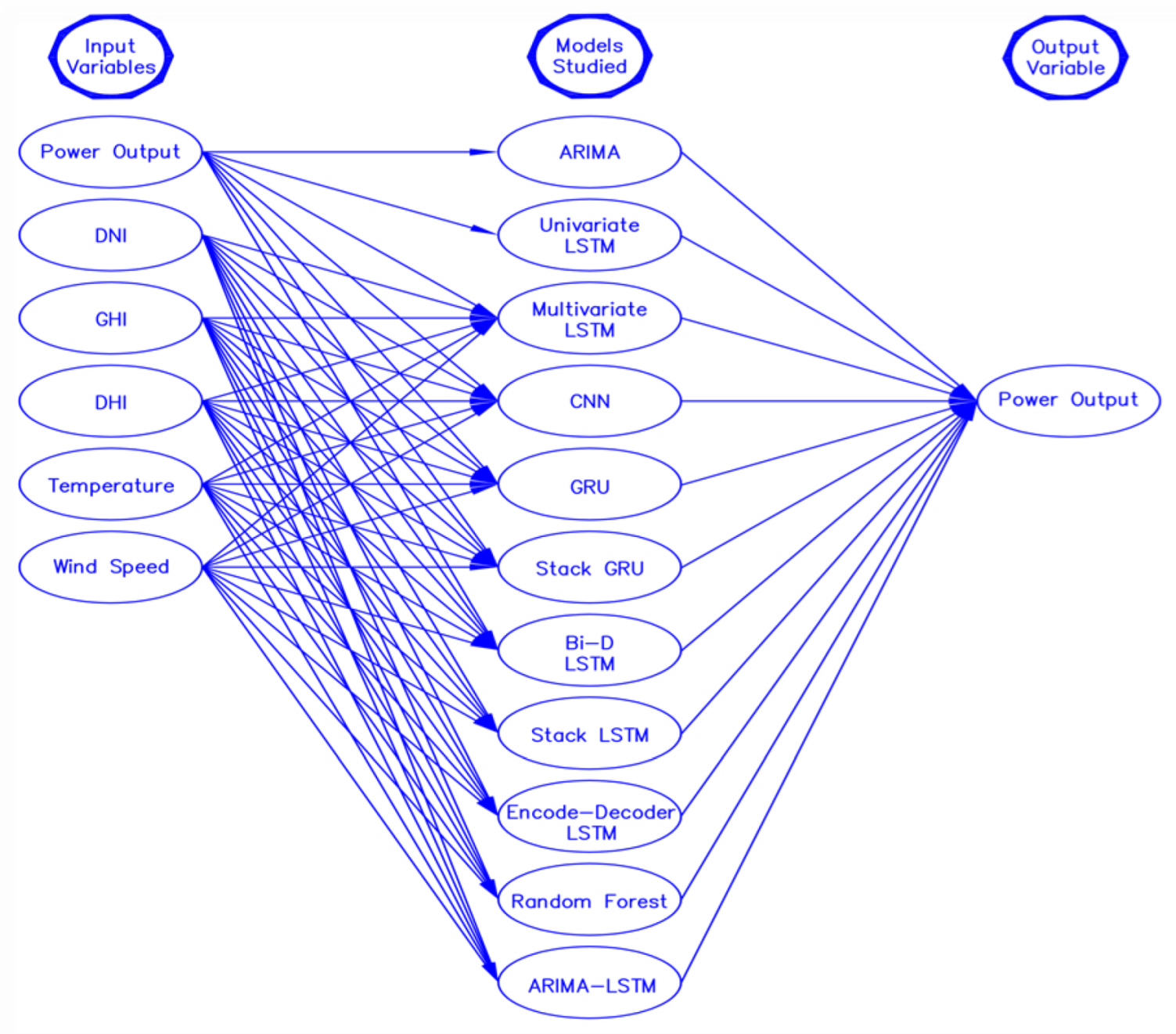
  • This study aims to provide a comprehensive comparison of popular forecasting models for long-term solar power generation forecasting, an area where there has been limited research.
  • The study seeks to understand the relationship between the forecasting model’s input variables and forecasting accuracy.
  • The study investigates how the performance of different models changes as the prediction horizon changes.
  • The study compares the performance of hybrid and ensemble models to that of single models.
  • The study assesses the performance of statistical, ML, DL, and ensemble forecasting models when limited input variables and datasets are available.
As the limitations of empirical-based forecasting models are discussed in Section 2, this study is significant in its examination of the limitations of models that have been in practice for decades, before comparing the performance of more recently developed forecasting models. The study, based on a case study conducted on a 100-kW solar power plant, aims to evaluate the performance of 11 different forecasting models and provide insights on how to improve their accuracy for long-term forecasting of solar power generation.

2. Limitation of the Existing Empirical-Based Forecasting Model

Prior to the introduction of the ML/DL model, the only way to efficiently determine the amount of global solar irradiation at any site was by installing measuring instruments such as a pyranometer and pyrheliometer at that place and monitoring day-to-day recording, which is a costly exercise [12]. Many developing countries cannot afford such instruments to accurately estimate solar irradiation at any location, which is why several correlations and methods have been developed in the past to estimate daily or monthly global solar irradiation [13,14]. Such correlations-based models and their application method is termed as empirical based model. The correlation models are based on geographical factors (latitude, longitude), astronomical factors (solar constant, solar declination hour angle etc.), and meteorological factors (temperature, sunshine hours, relative humidity, etc.) [15]. The most common empirical models are the sunshine- and cloud-based models.

2.1. The Sunshine-Based Model

The sunshine duration and clear sky radiation data are utilized as a parameter to predict the solar radiation at any time/day in the sunshine-based model. Angstrom–Prescott model is such a widely used model for calculating the monthly average daily radiation (H).
Were,
H H 0 = a + b S S 0
The monthly average extraterrestrial radiation ( H o ) can be calculated using Equation (2):
H o W h m 2 d a y = 24 π I s c 1 + 0.033   c o s 360 n 365 c o s Ø c o s s i n ω s + π 180 ω s s i n φ s i n δ
where parameters , ω s , S , S 0 , Ø , φ ,   a , b is solar declination, sunrise hour angle, monthly average daily sunshine duration, the monthly average daily maximum possible sunshine duration, solar zenith angle, the latitude of the location, and correlation coefficient respectively [15]. Similarly, Isc and n are referred to as solar constant (1367 W/m2) and the number of days starting from 1 January, respectively.
Despite the popularity of the Angstrom-Prescott model, the model fails to accurately predict solar irradiation due to dependencies upon many meteorological factors and the inability of the model to incorporate cloud covering [16,17]. Similarly, there are several other sunshine-based regression models based on Angstrom–Prescott model where the only difference between these models is the value of coefficients which are location dependent [18]. Some of the models are:
Katiyar et al. [18] model for India
H H 0 = 0.2281 + 0.5093 S S 0
Jain model for Italy
H H 0 = 0.177 + 0.692 S S 0
Li et al. Model for Tibet, China
H H 0 = 0.2223 + 0.6529 S S 0
All these models are dependent on multiple variables and have been used to compute the solar irradiance at different locations by modifying the coefficients of the Angstrom-Prescott model. As the coefficients are dependent on place and time, it follows that the sunshine-based model cannot be applied equally over the globe. The research conducted by Junliang Fan et al. [19]. in various regions of China revealed that the machine-learning model surpassed the empirical sunshine-based model, which serves as the foundation for this investigation into determining the most effective ML/DL models for long-term solar power forecasting.

2.2. The Cloud-Based Model

The most significant atmospheric phenomenon limiting the availability of solar energy on the earth is cloud cover and weather patterns. So, by collecting various data using the meteorological satellite and identifying the cloud patterns, the cloud-based forecasting model was developed with the intention to overcome the limitation of the sunshine-based model [20]. The cloud-based model certainly has the advantages over the sunshine-based model, in that its application is not geographically constrained and no physical solar radiation measuring instruments are required. Paltridge model developed by Paltridge and Proctor [21] is the most popular cloud-based model where parameters like solar zenith angle θ , and cloud factor CF are used to estimate the hourly diffused radiation ( I d ) and hourly beam radiation ( I b ) ,
Where,
  I b = 3.42286 1 exp 0.075 90 θ ]
  I d = 0.00913 + 0.0125 90 θ + 0.723 CF
And total radiation is calculated using Equation (8):
H = 1 CF Sunrise Sunset I b θ cos θ dt + Sunrise Sunset I d θ dt
Although the cloud-based model was frequently used for solar irradiance forecasting, it is no longer the favored method owing to the expensive cost of getting the necessary parameters and the model’s inability to predict the long-term forecast [22]. All empirically based models, not just those based on sunlight and clouds, are incapable of accurately predicting solar irradiance and solar energy output in noisy environments due to their inability to account for complex and nonlinear correlations between independent variables and dependent variables [23]. Several studies have shown that the ML/DL model is more accurate and cost-efficient than the empirical/physical-based model [24,25,26]. The ML/DL models’ ability to accurately estimate solar irradiance with just one input parameter makes them a better choice for predicting solar irradiance/solar power production. Therefore, this study investigates the usefulness of several statistical, ML, and DL models with the aim of enhancing long-term forecasts of solar power output. The significance of data processing approaches, the best fit model, and feature engineering that improve forecasting performance are emphasized in this study.

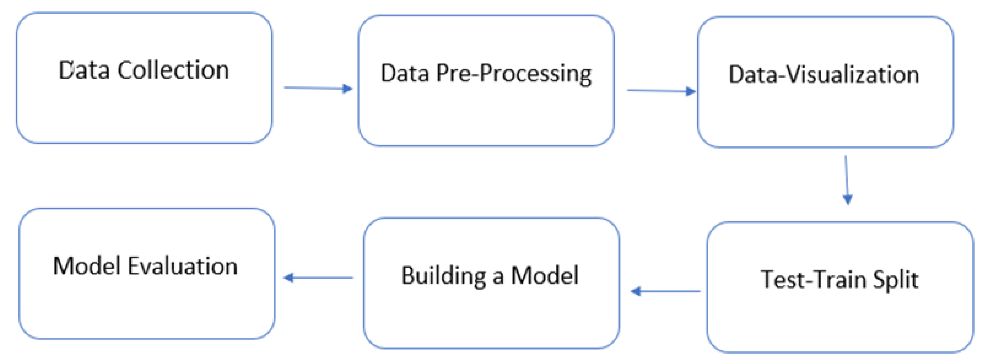
3. Materials and Methods

The first step in the methodology of this study is data collection, which is followed by data preprocessing and Exploratory Data Analysis (EDA) to verify the accuracy of the collected data. After the data preprocessing step, univariate and multivariate statistical, ML and DL models are tested with a 100-kW solar power plant’s hourly power production data. Firstly, the performance of three different univariate models is tested. The best-performing univariate model is re-analyzed with additional input variables to understand how the accuracy of the model changes with the change in the numbers of the input variables. Further, ensemble models are tested with the same datasets to see if the amalgamation of the models increases the prediction accuracy. Lastly, the optimal model is selected for predicting long-term solar power forecasting for the case study plant. The flowchart of the methodology of the study is presented in Figure 1.

3.1. Data Collection

For this study, one-year hourly global irradiation data are imported from National Solar Radiation Database (NSRDB) which is a NREL database (station 565910) [27]. Using the imported data, a 100-kW solar power plant is designed for the Lubbock Texas region using SAM [28] software (online opensource NREL’s software version 2022). An hourly one-year solar power production data (kWh) from a modeled power plant is imported to perform a statistical, ML and DL model to predict solar power production for the next 1 day, 3 days, 5 days, and 15 days. The solar power plant is designed for a location with an altitude of 983 m, latitude 33.57° N, and longitude −101.86° E. The Figure 2 shows different input variables and models that are utilized in the study.

3.2. Data Pre-Processing

The ability of the ML/DL model to learn is directly impacted by the quality of the data, hence it is critical that we preprocess the data before introducing it to the model. Data preparation is the process of getting the raw data ready (clean and organized) so that it can be used to create and train different ML/DL models. To put it simply, data preprocessing is a data mining approach that converts unstructured data into a format that is legible and intelligible to the ML/DL models. In this study, we have used weather data (DNI, GHI, DHI, temperature, wind speed, and power output) at a frequency of 1/3600 HZ. Here, DNI is Direct Normal Irradiance, GHI is Global Horizontal Irradiance, and DHI is Diffused Horizontal irradiance. The data preprocessing for the study includes handling missing data, outliers, and noise, data scaling, one hot encoding, etc. The stochastic regression imputation technique is implemented to impute the missing data and replace the outliers and noise in the data.

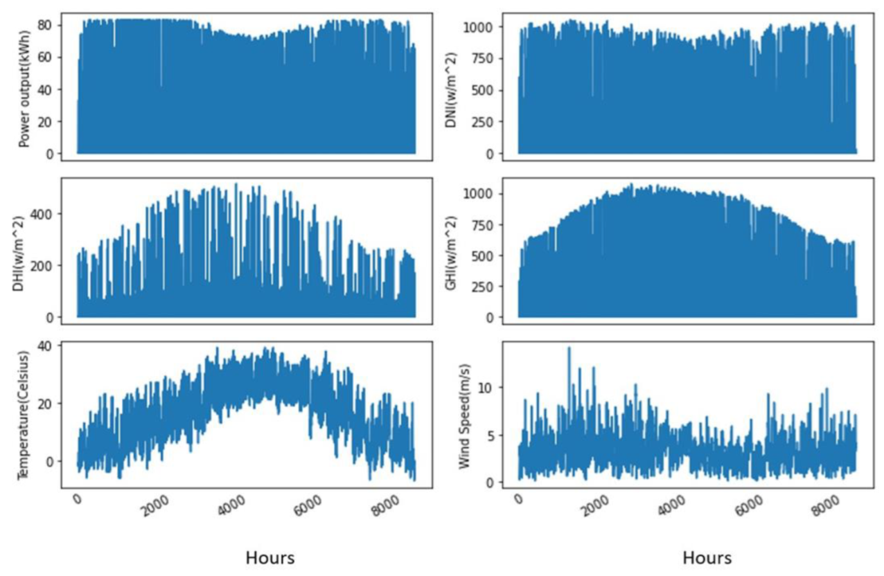
3.3. Data Visualization

Data visualization tools offer a simple approach to spotting and comprehending trends, data patterns, and outliers. Tools and methods for data visualization are crucial for processing large amounts of information and making data-driven decisions. For this study, the python package Matplotlib [29] is used to visualize the data. Figure 3 represents the graphical representation of different data utilized in the study.

3.4. Test-Train Split

The accuracy of every prediction model can be determined by the model’s performance analysis, for which test data are required. The test dataset cannot be the same as that used for training the model. Hence, the essential step in any ML/DL modeling is to split the data into train and test sets. Sometimes some portion of the test set can be used to validate the model as well and which is known as a validation set. In this study, about 70% of the data are used for training, 20% for validation, and 10% for testing.

3.5. Building a Model

In this part, the literature and methodology of implementation of different (statistical, ML, DL, and ensemble) models are analyzed and compared for both the univariate and multivariate datasets. A detailed comparison is available in Section 4. However, in brief, the following Section 4 first compares the univariate models, namely, ARIMA, SVR, and univariate LSTM in Section 4.1, which are statistical, ML and DL models, respectively. The best-performing model out of the above three models is re-analyzed in Section 4.2 with addition of input variables. Later, in Section 4.3, the best-performing model and worst-performing model from 4.1 and Section 4.2 are ensembled to see how the prediction accuracy change with this combination. The results are summarized in Section 5. Lastly, a discussion of the results obtained is presented in Section 6.

3.6. Model Evaluation

The accuracy of the models has been compared using the RMSE (Root Mean Square Error) test. The RMSE test is used to identify the difference between an observed value and the predicted value. The RMSE value ranges from 0 to infinity. The accuracy of the model with an RMSE value near 0 is the highest [30].
R M S E = s q u a r e   r o o t i = 1 n Y i Y j Y i Y j n
where Yi corresponds to the actual value and Yj is the forecast value.
The impact of the prediction horizon, the number of input variables, feature engineering, data processing, and ensemble models are summarized in this part of the study.

4. Building a Model

4.1. Univariate Models

As mentioned in the methodology Section 3.5, a univariate model for each of the three types of models—statistical, ML, and DL—is tested in this section. The univariate dataset utilized in the analysis is hourly year-long solar power production data from a 100-kW solar power plant. Firstly, a statistical model (ARIMA) is implemented after data are pre-processed by removing noise and outliers. Then, the stationary data are checked by examining Auto-Correlation Function (ACF), and Partial Auto-Correlation Function (PACF) test, and then seasonality/non-seasonality, trends, etc. in data are checked to choose the correct ARIMA algorithm. ARIMA (p, d, q) model is built based on the lowest values of the Akalike Information Criterion (AIC). The methodology of forecasting using the ARIMA model is presented in Figure 4. Secondly, the univariate SVR algorithm is tested on the same datasets by importing SVR libraries in the python keras package. Then, Radial Base Function (RBF) is chosen as the kernel to standardize the data between the values 0 and 1. Then, SVR parameters are chosen based on the trial-and-error method. Finally, the correlation matrix is determined to identify the relationship between the time stamp input variable data and prediction is made thereafter. Lastly, the deep learning algorithm, LSTM model, is run for the same datasets after scaling the datasets using activation functions like a sigmoid (σ) and hyperbolic tangent function (tanh). The LSTM model is tuned by changing various parameters such as changing the number of LSTM layers, adding dropout value, increasing the number of epochs, changing optimizer type, varying batch size, etc. to yield maximum accuracy. The results of the comparison of the above-mentioned models are presented in Section 5.1.

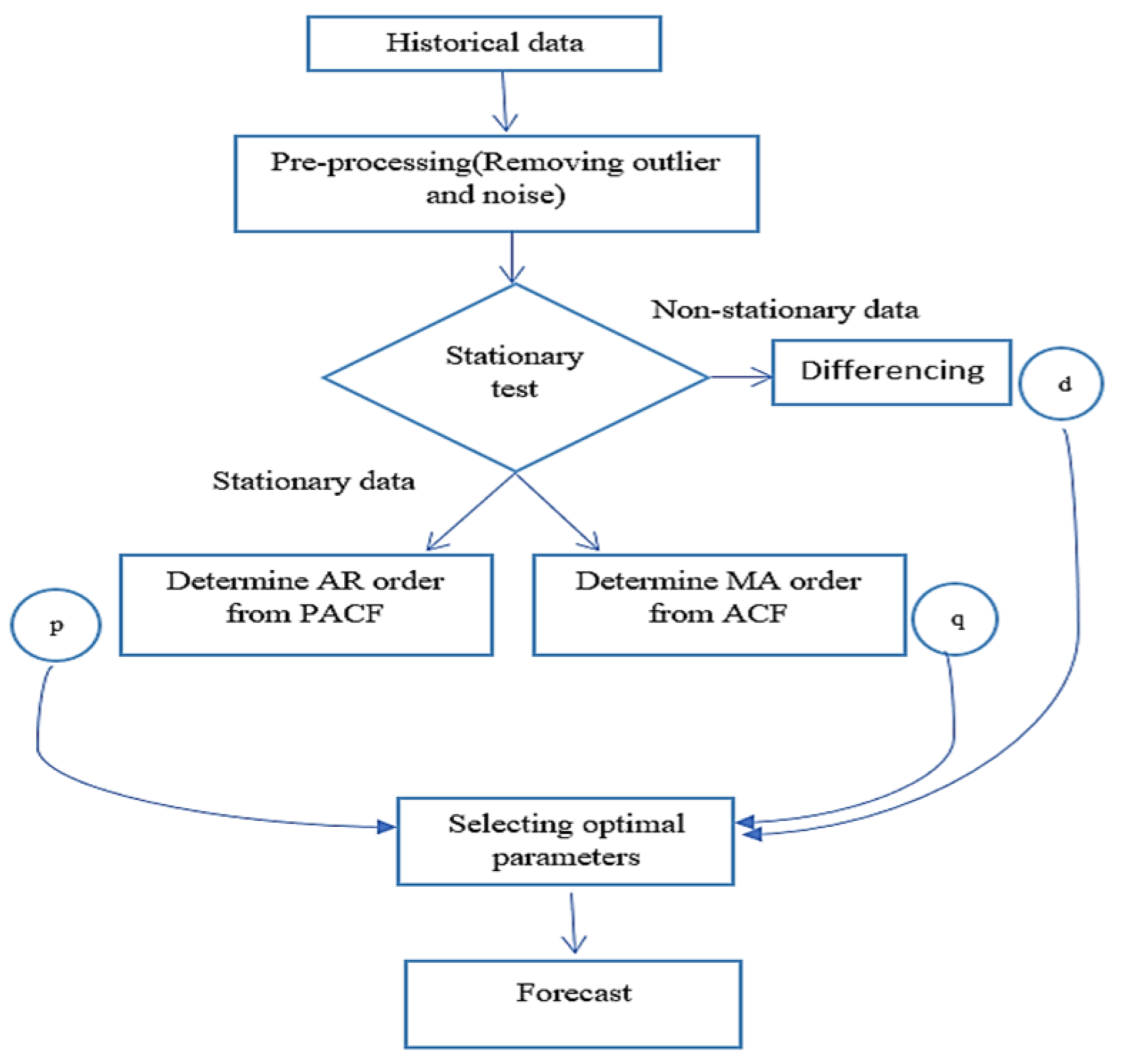
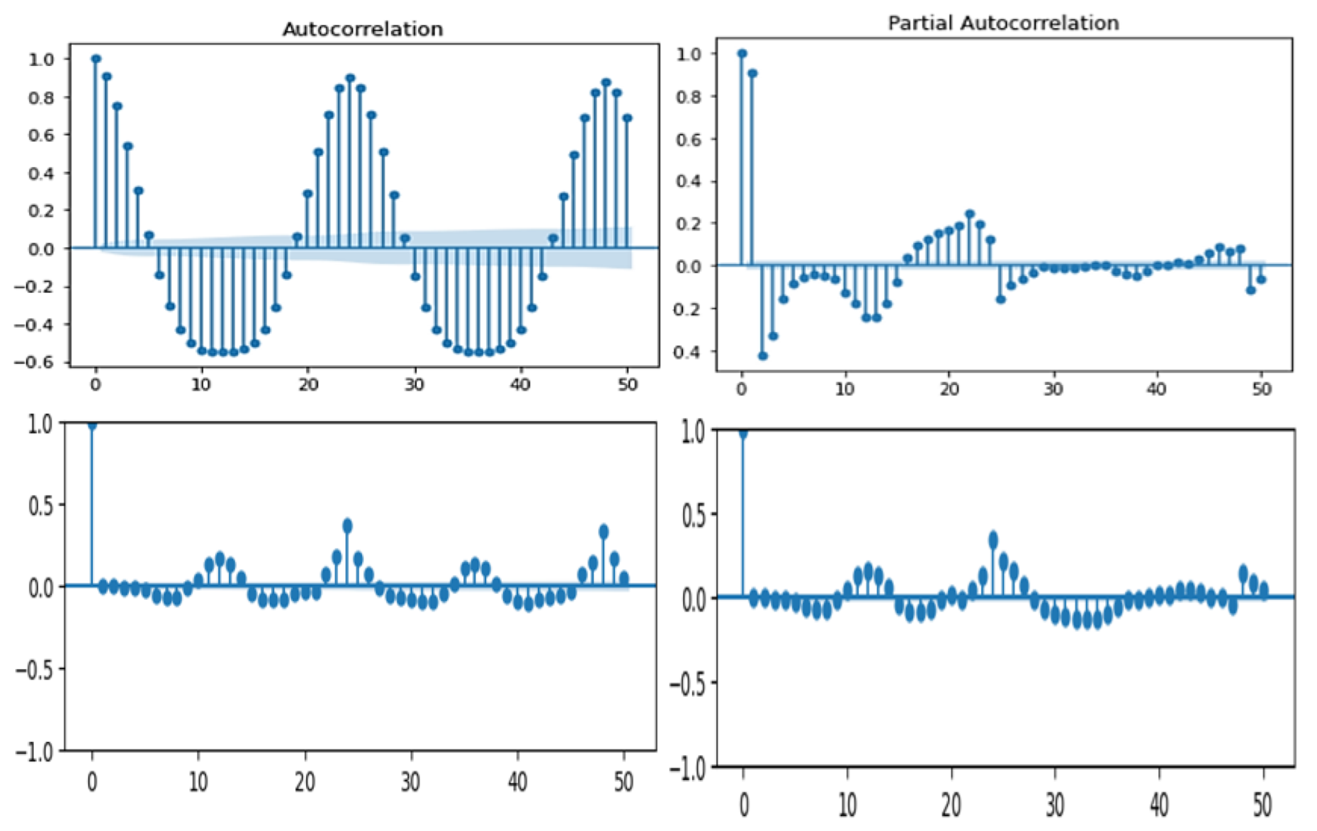
4.1.1. Statistical Model (ARIMA)

Autoregressive models are those that predict future features based on prior attributes. The ARIMA model is a developed version of the basic Autoregressive Moving Average (ARMA) model with the introduction of the Integration term(I) [31]. The ARIMA model is a type of statistical model that merely requires historical data to understand the pattern and make a prediction. This simple yet efficient method of forecasting is of regression analysis type normally used for the data that demonstrate stationarity nature. In ARIMA, the term AR, I, and MA represents the following responsibilities. AR (Auto-Regressive) model is responsible for understanding the correlation between the observed value and its lagged value. I (Integrated) model is responsible to make the best fit of data by substitution of data with the differenced term (observed value-its lagged value) [32]. MA (Moving Average) model is responsible for understanding the correlation between an observed value and a residual error in the lagged data. Each of the above terms is associated with the parameters represented as (p, d, q), in which:
  • p: corresponds to the quantity of lag observation in a model.
  • d: corresponds to the number of times the observed value is different from its lagged value.
  • q: corresponds to the order of lagged prediction error.
  • Seasonality versus non-seasonality
ARIMA models for seasonal and non-seasonal data are different. Seasonality is the existence of a consistent trend in the historical time series data.
The non-seasonal ARIMA [33] model evaluates time series data using Equation (10):
y t = μ + ϕ 1 y t 1 + + ϕ P y t p AR   terms θ 1 e t 1 θ q e t q MA   terms
where, μ is constant, θ   and   ϕ are model parameters of MA and AR terms respectively, yt is time series, p, d, and q are non-seasonal ARIMA parameters, and et is the white noise.
The seasonal ARIMA model [33] is similar to the non-seasonal ARIMA model with an addition of a backshift operator (B) term to achieve convenience in describing the process of differencing in time series data. Where B is
B = yt−1
The seasonal ARIMA model evaluates time-series data by multiplying seasonal parameters with non-seasonal parameters as:
(p, d, q) ∗ (P, D, Q) ∗ m
where m is the number of observations and P, D, and Q are seasonal AR, MA, and I order respectively. Seasonal ARIMA is chosen for this study due to the seasonality in the training datasets.
  • Stationarity of the data
Time series data are said to be stationary if the mean does not vary over time and the variance is zero. Statistical modeling methods like ARIMA presumes or require the time series data to be stationary to project an accurate prediction. Different ways to test the stationarity of the time series data are to perform an Autocorrelation Function (ACF) test, Partial Autocorrelation Function (PACF) test or Augmented Dickey-Fuller (ADF) test. For this study, ACF and PACF test is performed to check the stationarity of the data. The data for this study is found to be stationary.
  • Determining p, d, and q parameters
Parameters are set by determining the values of the model coefficients that offer the best representation of the data using maximum likelihood or minimal least square approaches. Models with the lowest Akaike information criterion (AIC) or Bayesian information criterion (BIC) are chosen. For this study, the least AIC value is evaluated to identify the optimal model [34].
AIC = −2 log (maximum likelihood) + 2 k
k is a number of independent parameters.
It is hard to quantify all three parameters (p, q, d) just by looking through ACF and PACF plot, however, this graph (Figure 5) gives some preliminary ideas. The plots of the ACF and PACF of the ARIMA model, which is used to identify the appropriate values for the model’s parameters such as the number of Auto-Regressive (AR) and Moving Average (MA) terms, are displayed in the top row of Figure 5. The plots for the residual ACF and PACF are similarly displayed in the second row. The similarity in the residual ACF and PACF plots suggests that the model may not be capturing all the patterns in the data. This highlights the need for either more data or a more accurate model to improve the model’s performance and its ability to make long-term forecasts. In both the graphs in Figure 5 (top row), the first few spikes are the most distinct and significant. This gives us the idea that p value is more than 1. Similarly, q can be estimated roughly from the ACF plot by looking at the number of lags crossing the threshold zone. However, to precisely quantify the parameters, the minimum AIC value is calculated by changing the (p, q, d) value. For this study, optimal parameters are (p = 3, q = 0, d = 5) with a minimum AIC value of 64,544.

4.1.2. The Machine Learning Model (SVR)

The Support Vector Regression (SVR) model demonstrates superior performance prediction compared to other ML models such as Linear Regression, (K-Nearest Neighbors) KNN, and Elastic Net [35]. This is because it has enhanced optimization techniques for a wide range of variables. Additionally, it is adaptable in how it handles geometry, transmission, data generalization, and kernel extensions [19]. By considering the quality of characteristics, this added capability improves the model’s ability to make predictions. For these reasons, SVR is the model of choice for this study. Drucker et al. first presented SVR, which is a supervised learning approach based on the support vectors theory of Vapnik [36]. The objective of SVR is to reduce error by finding the hyperplane and decreasing the difference between expected and observed values. The Support Vector Machine (SVM) serves as the foundation for the SVR method. SVR is a regressor used to forecast continuous ordered variables, in contrast to SVM, which is used to predict discrete categorical labels. The objective of simple regression is to minimize error rates, but the objective of SVR is to fit the error inside a preset threshold. This suggests that the objective of SVR is to approximate the optimal value within a specified margin known as the epsilon tube, which ranges from positive to negative epsilon as seen in Figure 6.
When using the SVR model, a nonlinear boundary must be built if the training data cannot be partitioned into independent subsets using linear means. By projecting the input space onto a higher-dimensional space known as feature space, the nonlinear boundary may be attained. The instances that share the same feature space are then searched for a hyperplane that can divide them. A kernel function defines the mapping between the input space and the feature space. The following sections explain the basic terminology involved in the SVR model.
  • Terminologies
    1.
    Hyperplane
The continuous output may be reliably predicted with the use of hyperplanes, which are decision boundaries. The data points that are located on each side of the hyperplane and are in the closest proximity to the hyperplane are referred to as Support Vectors. These are what is needed to draw the necessary line that demonstrates the expected result of the algorithm.
  •  
    2.
    Kernel
Kernels are mathematical functions that transform data into the desired form (like, 0 to 1, −1 to 1, etc.) and are used to discover a hyperplane in higher-dimensional space.
  •  
    3.
    Support Vectors
Support vectors are data points that are nearer the hyperplane and have an impact on the hyperplane’s position and orientation.
  •  
    4.
    Boundary lines
The boundary line is the point where two parallel lines drawn to the two sides of the Support Vector meet and the error threshold value, epsilon, is exceeded. These lines demarcate a space around each data point.
  • Importing libraries and training dataset
The SVR analysis prepackaged library in Python is utilized in this investigation. To assess the model’s performance, 8760 data points representing hourly solar power output data are used. The split of the dataset between training, validation, and test set is 70%, 20%, and 10% of the total datasets respectively.
  • Selection of Kernel
The Sigmoid Kernel, Polynomial Kernel, Gaussian Kernel, Radial Basis Functions (RBF), etc. are all examples of kernels often used in SVR analysis [37]. Since the RBF kernel is the most often used kernelization method due to its proximity to the Gaussian distribution, it is used in this study [38]. The RBF kernel is flexible enough to handle both linear and non-linear input-output mapping, and it has fewer hyper-parameters to tune than kernels like the polynomial kernel, reducing the computational cost of finding the optimal hyper-parameters. Additionally, the RBF kernel’s values are constrained to lie between 0 and 1, resulting in fewer numerical difficulties than the polynomial kernel’s, which can lie between 0 and infinity [39].
  • Determining the SVR parameters
Three training parameters (kernel, C, and ε) for an ε-insensitive loss function affect how well the SVR method performs. However, the complexity of the resulting model is sensitive to the values of C and ε for any kernel. The prediction accuracy may be improved by increasing or decreasing the number of Support Vectors (SV). The less complicated the regression estimates are, the larger they should be set to. However, C’s value is the compromise between the ease with which the model can be understood and the tolerance for error in the optimization method [40]. For this study, C = 10, epsilon = 0.05 is chosen based on the trial and error that results in minimum prediction error.
  • Correlation matrix and predictions
Lastly, the correlation matrix is formed based on the parameters like Kernel, C, and ε, which are responsible for making predictions of future values.

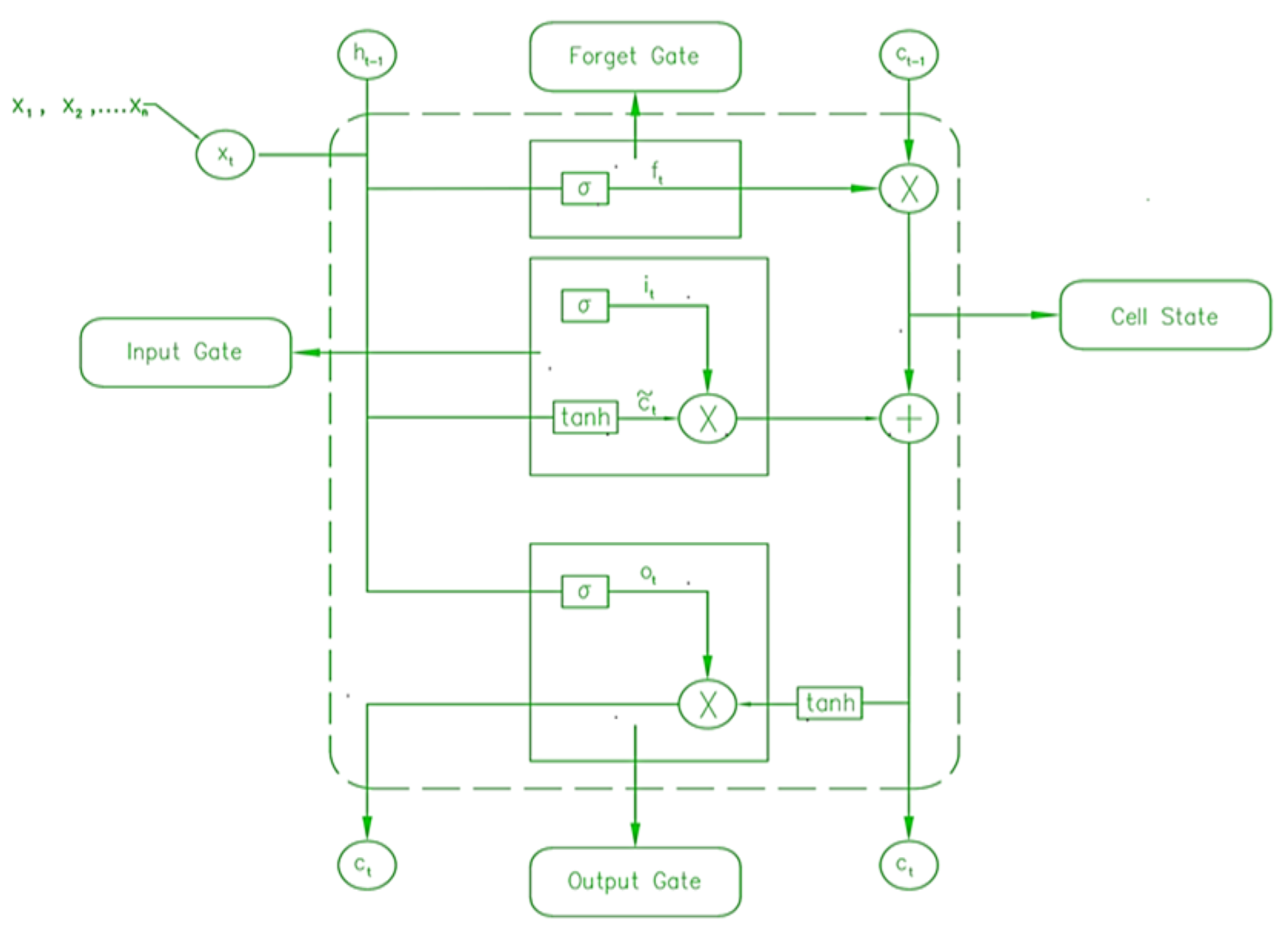
4.1.3. Deep Learning Model (LSTM)

To overcome the vanishing gradient problem in handling long-term sequences in Recurrent Neural Network (RNN), advance RNN models, i.e., the LSTM model is developed which has a similar structure as RNN but has different inner cells [41]. The LSTM model is equipped with the ability to utilize memory blocks to store and transfer information for a long period and reduce the rate of data loss [42]. Each unit in a block consists of three types of gates for controlling the memorizing process as represented in Figure 7.
  • Gates
    1.
    Forget gate
Forget gate is the first gate in LSTM architecture where information is either forgotten or stored based on the significance of information to the result. The forget gate is supposed to read and store information on current input (Xt) and previous layer output (yt−1), and to apply the sigmoid activation function (σ) on the available information. The activation function results in a value of forget gate (ft) into a binary value (either 0 or 1) [43]. The value of ft being 1 means remember every piece of information, and the value of ft being 0 means forget every piece of information. Forget gate (ft) is calculated as
f t = σ w f . y t 1 , x t + β f
In Equation (14), Wf is the weight matrix between forget gate and input gate where information is either stored or forgotten, and β f is the gate layer’s bias term.
  •  
    2.
    Input gate
The input gate is the second gate in LSTM architecture where the significance of the new information carried by the input is evaluated. It is divided into two sections. First, the previous hidden state (Ht−1) and current input (Xt) are sent to the sigmoid activation function ( σ ) to determine which values will be updated. Then, to govern the network, the same two inputs are fed into the tanh activation function. Finally, the tanh output (Ct) is multiplied by the sigmoid output (It) to determine which information is critical for updating the cell state [1]. Input gate (It) is evaluated as,
It = σ(Xt × Ui + Ht−1 × Wi)
Ht = It × tanh (Ct)
In Equation (15), Wi is the weight matrix of the sigmoid operator between the input and output gate and Ui is the weight matrix of the input.
  •  
    3.
    Output gate
The output gate is the final gate in LSTM modeling where, previous input information is reviewed, and forecasting is made based on that information. The prior hidden state (Ht−1) and current input (xt) are both sent to the sigmoid activation function, much as the input gate. After going through the sigmoid function, the output is multiplied by the output of the hyperbolic function (tanh) to yield the current hidden state (Ht). The final outputs are the current state (Ct) and the present hidden state (Ht). The following equation governs the output gate [44].
Ot = σ(Xt × Uo + Ht−1 × Wo)
Ht = Ot × tanh (Ct)
where Wo is the weight matrix of the output gate and Ui is the weight matrix of the input.
To summarize, the forget gate determines which preceding information is important. The input gate determines what relevant information from the current phase may be added, and the output gate finalizes the next hidden state and provides the desired output.
  • Execution steps
The default univariate LSTM model available in the Keras package in Jupiter Notebook [45] is utilized for this study. The same dataset as ARIMA is utilized in this model. Hourly one-year PV output data are divided into training and testing datasets after removing noise and outliers in the data, where 90% of the data are utilized for training purposes and 10% of the data are utilized for testing purposes. The normalization method is applied to datasets, which standardized the data into binary values (0 and 1), making the model easier to interpret. Similarly, four distinct hidden layers are investigated, and the best fit out of the four different models is evaluated using different precision approaches. The number of neurons in this study has been kept fixed for all the datasets. Similarly, optimizers are used to increase the accuracy of the model.
  • Network Architecture
Several activation functions like Sigmoid, SoftMax, and Rectified Linear Unit (ReLU) can be implemented in the LSTM model to standardize the dataset value between −1 to 1 to better interpret the result [46]. For this study, the sigmoid and hyperbolic tangent activation function is implemented. Similarly, optimizer algorithms are used for minimizing errors in the forecasting model [10]. An Adam optimizer is used in the model to efficiently handle sparse gradients in stochastic datasets [47]. To avoid the overfitting of the data in the model, drop-out layers are used. Drop out layer randomly enable/disable neuron and update memory cell in LSTM. To ensure accurate forecasting, large epochs (30) and a small batches size (32) are chosen.

4.2. Multivariate Models

In this section, the best performing model of Section 4.1, i.e., the DL model (LSTM) is re-evaluated with the addition of new variables to understand how the accuracy of the model change with the change in the number of input variables. The results of the comparison of univariate models are presented in Section 5.1. Six distinct types of LSTM models are evaluated in this section with multivariate datasets.

4.2.1. Multivariate-LSTM

As the name suggests, this model incorporates multiple input variables like solar power output, DNI, GHI, DHI, Wind speed, and temperature and predicts the solar power production as output. The working principle of Multivariate LSTM is presented in Figure 8 below which is similar to the univariate LSTM model.

4.2.2. Stacked LSTMs

The stacked LSTM is an improvement to the multivariate LSTM model that includes several hidden LSTM layers (Figure 9) with numerous memory cells in each layer. The model becomes deeper because of the stacked LSTM hidden layers, more appropriately deserving of the label “deep learning approach”. In a stacked LSTM, the output of the first LSTM layer is utilized as the input for the second LSTM layer, which creates sequence vectors. The next LSTM’s input at time t + 1 receives the output of the LSTM at time t [48].

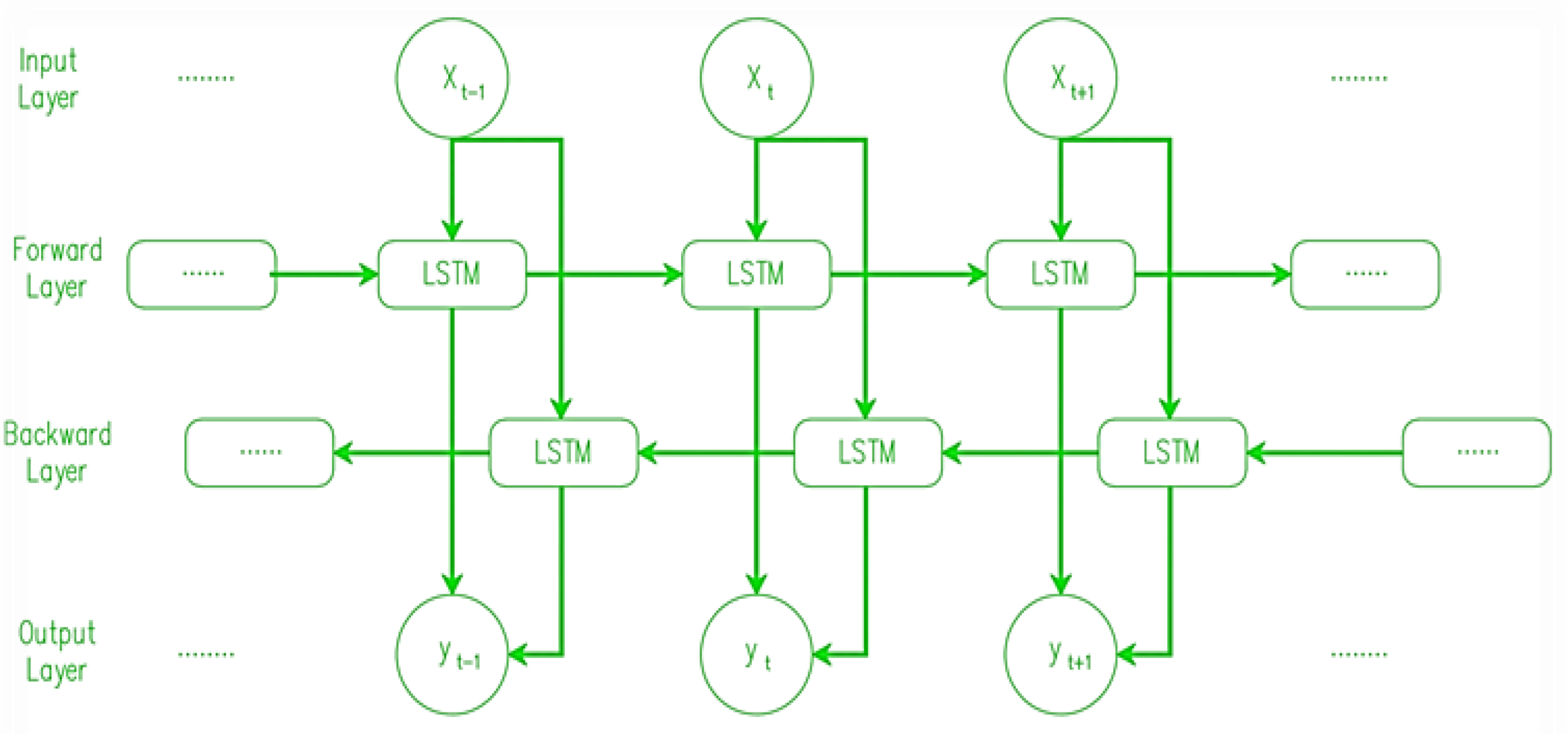
4.2.3. Bi-Directional LSTM

In addition to being an expansion of the multivariate model, bidirectional long-short-term memory allows for the transmission of data in both ways, either backward or forward (Figure 10). The conventional LSTM only allows for unidirectional input flow, in either direction. On the other hand, using bidirectionality, we can ensure that data are kept both in the future and in the past [49].

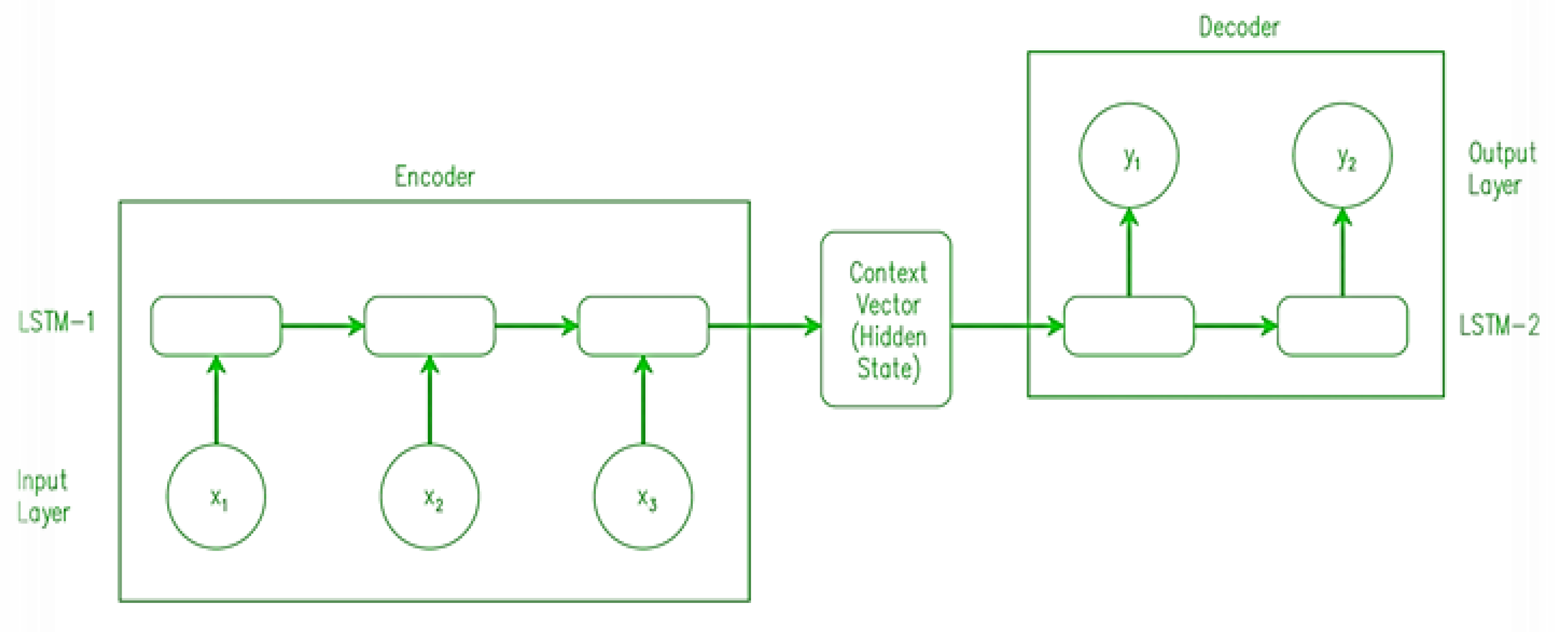
4.2.4. Encoder-Decoder LSTM
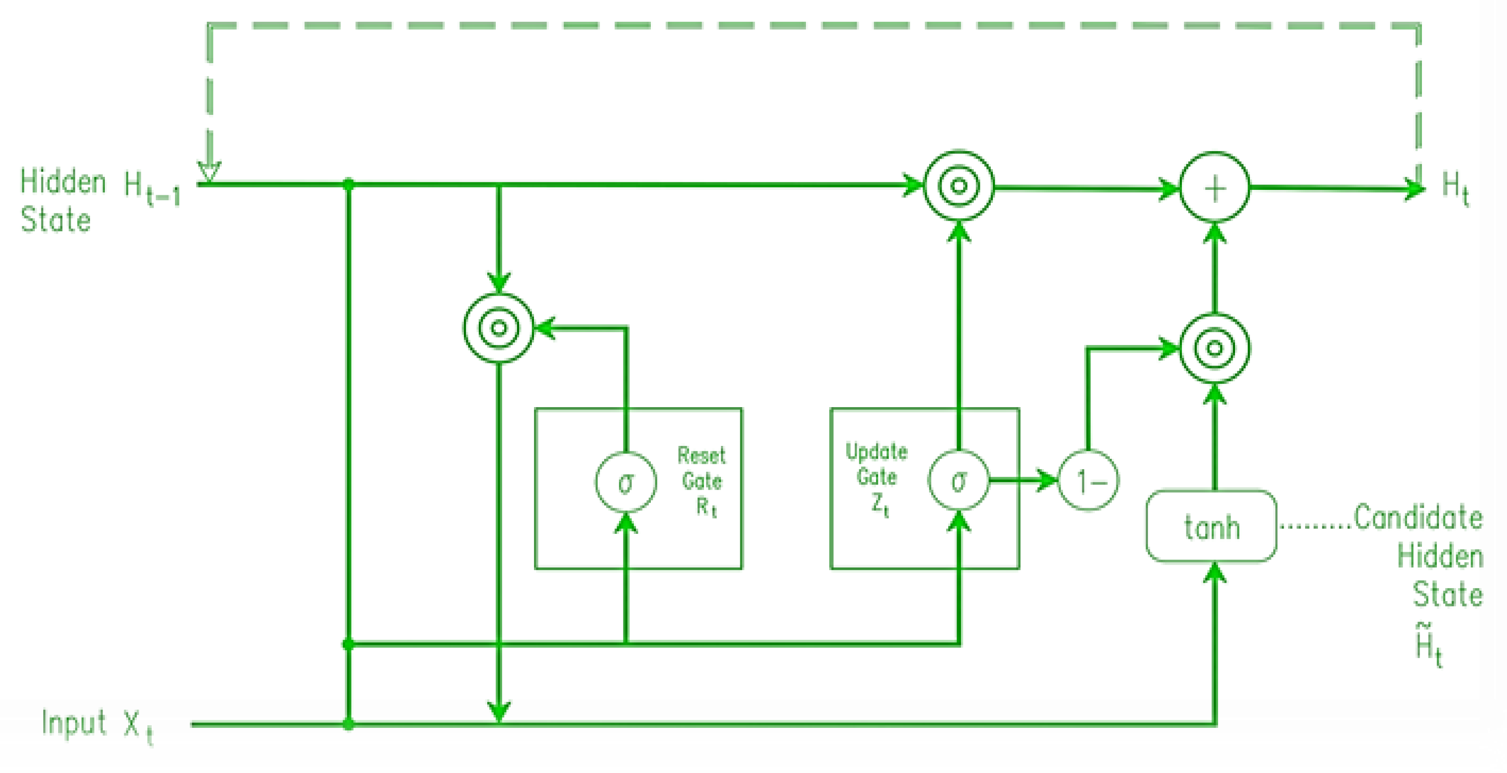
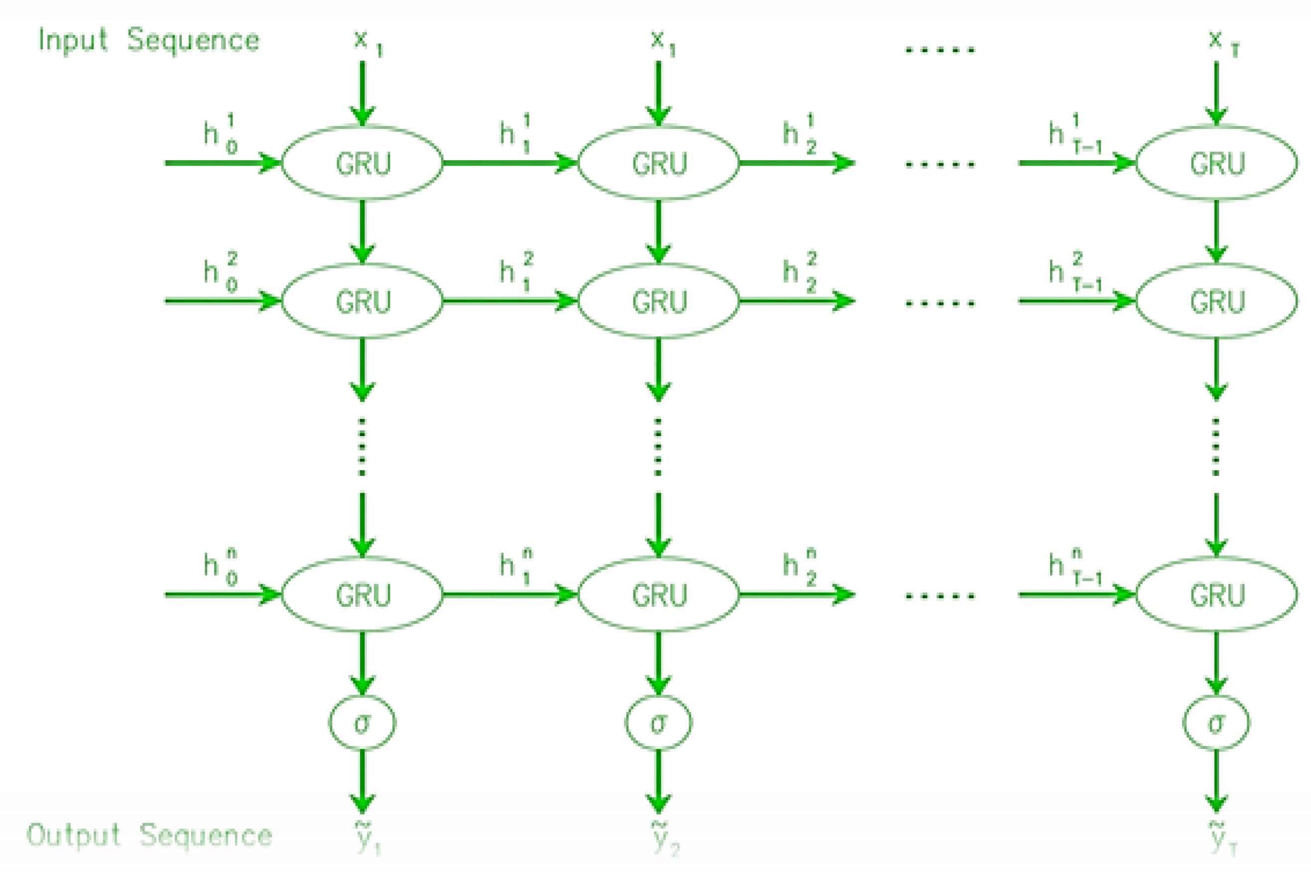
Both the encoder and the decoder are generally LSTM models. To enable the input sequence, an encoder creates a set of numbers called internal state vectors (in the case of LSTM, these are called the hidden state and cell state vectors). The states of the Decoder LSTM are initialized to match those of the Encoder LSTM’s output states. Decoder begins creating the output sequence using these starting states. The input sequence is first summarized by the encoder into state vectors (also called thought vectors), which are then sent to the decoder, which begins creating the output sequence based on the thought vectors [50]. Figure 11 depicts the above information in pictorial form.
The working architecture of GRU (Figure 12) is like LSTMs, but with two gates instead of three (a reset gate and an update gate). It is the job of the reset gate to decide how much of the prior state to retain, while the update gate decides how to mix the incoming input with the stored data. The input gate and forget gate of an LSTM have been replaced with an update gate in a GRU. Unlike the LSTM unit, the GRU unit does not need a memory unit to regulate data transfer. It has unrestricted access to all latent states and may utilize them directly. Since GRUs have fewer parameters, they could learn more quickly or with fewer data. However, LSTMs with more expressiveness may provide superior results with huge datasets. In addition, the vanishing gradient issue, which plagues most RNNs, is solved by GRUs [51]. The neural network may become untrainable if the grade becomes too tiny over time due to backpropagation. Two gates, the update gate and the reset gate, help GRUs deal with this issue. These gates are responsible for determining what data are sent to the output and may be taught to remember data from earlier in the chain. By doing so, it may improve its predictions by relaying information through a causal chain [52].

4.2.5. Stacked GRU

The stacked GRU is functioning like the stacked LSTM where the output of the first GRU layer is utilized as the input for the second LSTM layer, which creates sequence vectors. The next GRU’s input at time t + 1 receives the output of the GRU at time t. Stacked GRU is an improvement to the multivariate GRU model (Figure 13) that includes several hidden GRU layers with numerous memory cells in each layer [53].

4.3. Ensemble Model

The idea behind an ensemble model is to make the model more accurate by putting together several different forecasting models. The different methods of model composition are called “bagging”, “stacking”, and “boosting”. By averaging the results of several similar models with high variance, bagging can reduce variance. Boosting builds multiple models one step at a time to reduce bias and keep the variance small. In the same way, stacking is the process of using different forecasting models one after the other, where the predictions from each model are added to make a new feature [54].

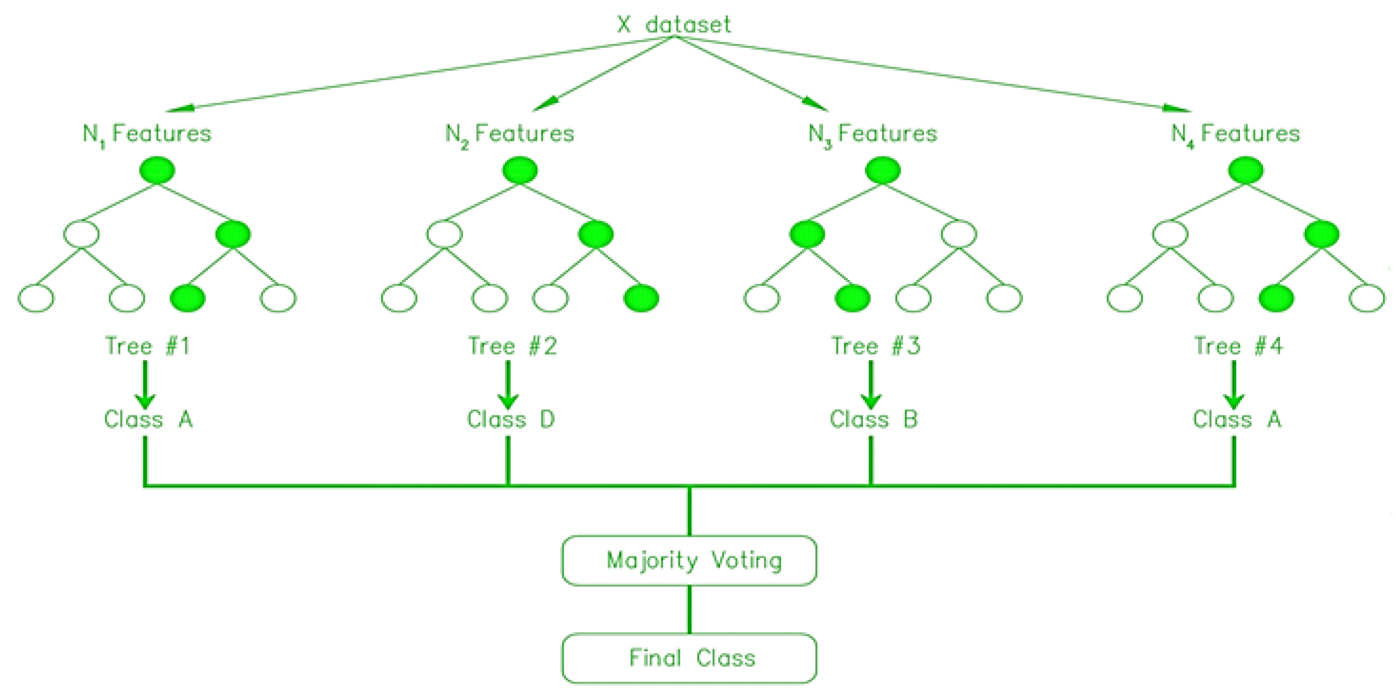
4.3.1. Random Forrest (RF)

RF regression is a supervised learning approach for regression that uses the bagging ensemble learning method. The random forest model is presented to improve the performance of the machine learning algorithm decision tree [55]. The issue with decision tree algorithms is that they tend to overfit smaller datasets [56]. This results in a large variance, which might be interpreted as high test mistakes on the test dataset despite the training dataset’s high accuracy. The RF approach resolves this problem by picking dataset features at random. This implies that RF will use a restricted amount of these qualities on each iteration. The output is ultimately selected depending on the results of each repetition with a separate subset [57]. One hundred Decision Tree (DT) results are gathered in this study. In Figure 14, only four DT trees are represented (for simplified representation of the model) where total datasets are divided into 4 different classes based on the N1, N2, N3 and N4 features.

4.3.2. ARIMA-LSTM

The study’s top-performing and bottom-performing models are combined to see whether there is a performance increase over separate models. To describe a linear relationship in time series paradigms, the ARIMA model works quite well [58]. In contrast, it is inadequate for modeling nonlinear connections. To counter this, the LSTM model may describe both linear and nonlinear relationships, albeit not all datasets will provide the same result [59]. Nonlinear and linear components of differential modeling were presented as part of the hybrid model idea for optimal prediction. In this study, the hybrid model is implemented first by removing the seasonal component in the dataset (Yt). To do this, we used the yt = mt + st + εt decomposition, the first phase of the ARIMA model. Three functions are obtained: trend mt, seasonal component st, and noise εt. To recreate seasonality, st and εt are kept, and εt is used to create confidence ranges for the projected values. Now that the datasets are devoid of seasonal variations, the datasets are passed to the deep learning model as input [60,61]. The remaining operation is analogous to the operation of the ARIMA and LSTM models separately.

5. Models’ Performance Comparison and Evaluation

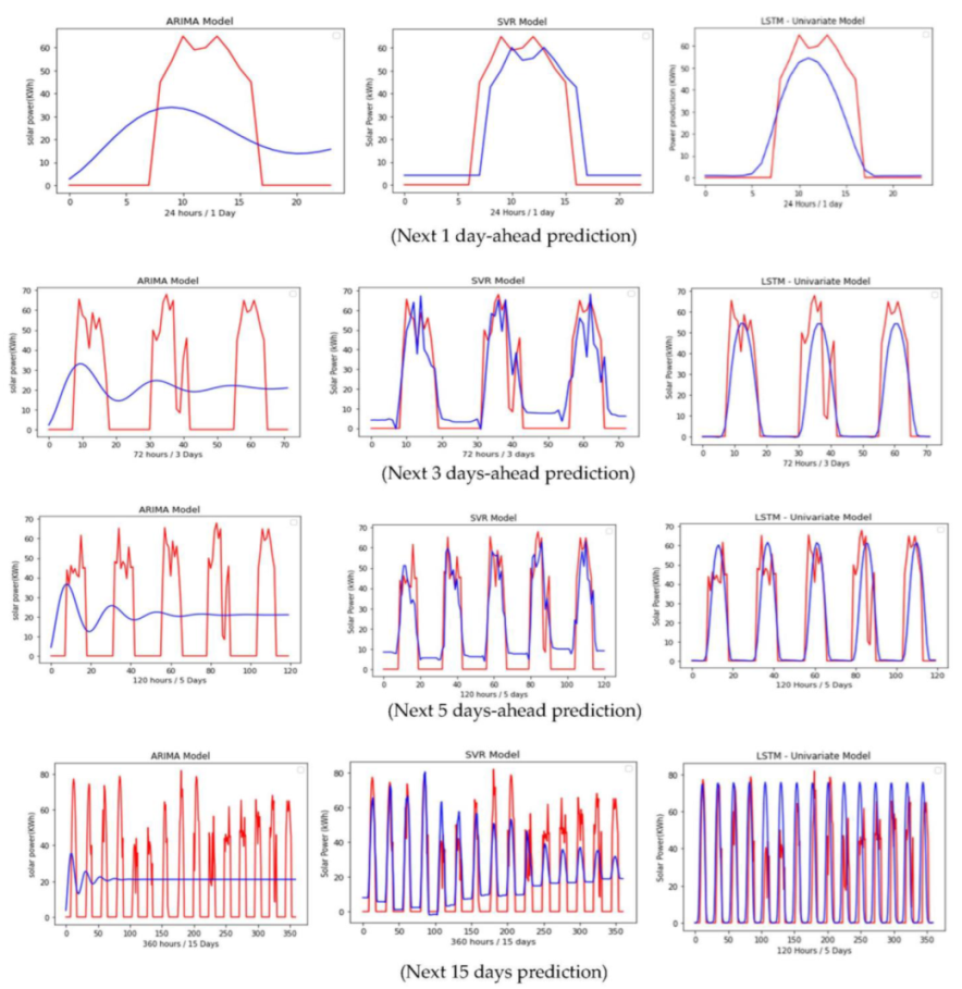
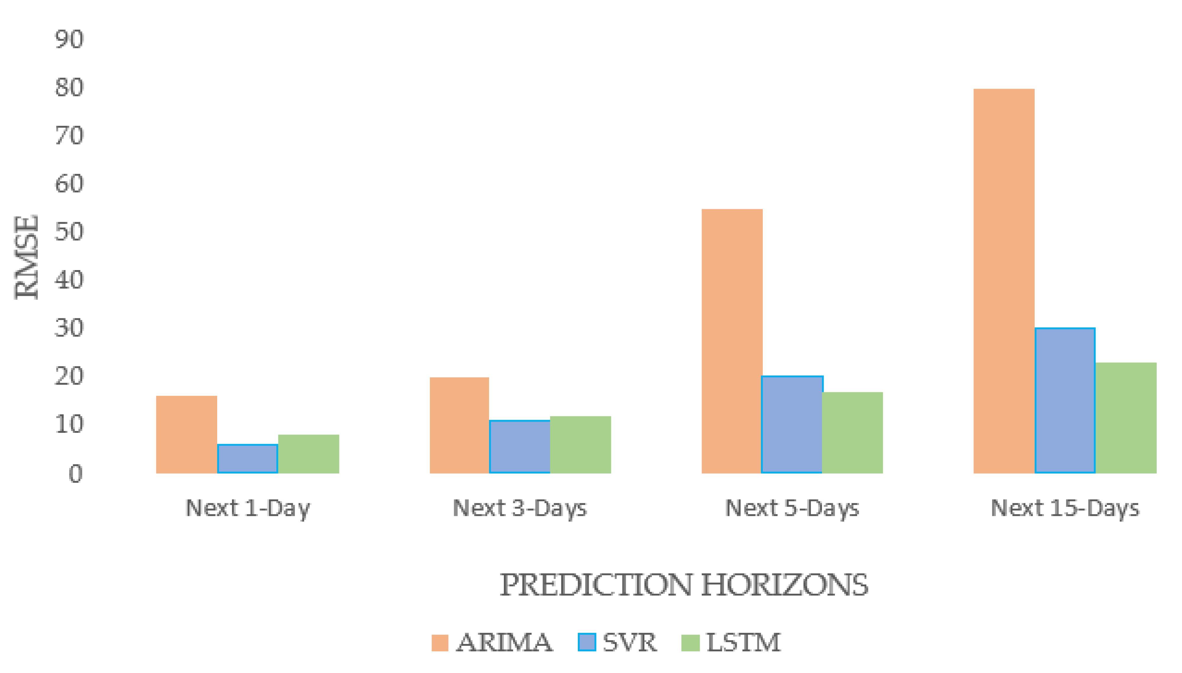
5.1. Comparison between Univariate Models (ARIMA, SVR, LSTM)

A comparison between three different models is presented in Figure 15 and Figure 16.
In terms of long-term forecasting of solar power generation, it is evident from Figure 15 and Figure 16 that the DL model (LSTM) performed better than the statistical model (ARIMA) and the ML model (SVR) for predicting the next 15 days-ahead solar power generation. The performance of the ML and DL models is found to be comparable; the ML model predicted the next 15 days’ solar power generation with an RMSE of 30 and the DL model predicted the same with an RMSE of 23. The statistical forecasting model was not as effective as the ML and DL models in capturing the intermittent behavior of solar power generation. Similarly, a significant reduction in the forecasting accuracy was observed in the statistical model (ARIMA) with an increase in the prediction horizon. On the other hand, the accuracy of ML and DL models is found to exhibit a gradual decrease in accuracy with an increase in the prediction horizon. Since the statistical model failed to accurately predict long-term solar power production, it is not advisable to use it for making long-term forecasts of solar power output. Although, ML Model (SVR) is found to exhibit better accuracy for predicting up to the next 5 days of predictions. The LSTM model is the better-performing model out of the three models (ARIMA, SVR, and LSTM) in this univariate model’s performance analysis, as the focus of the study is to analyze the efficacy of the model for its ability to accurately predict long-term forecasting (up to next 15 days). Though ML/DL models performed better, they have several drawbacks, such as overfitting on small datasets, a requirement for massive amounts of training data, a complex architecture, a need for more computational capacity, etc.

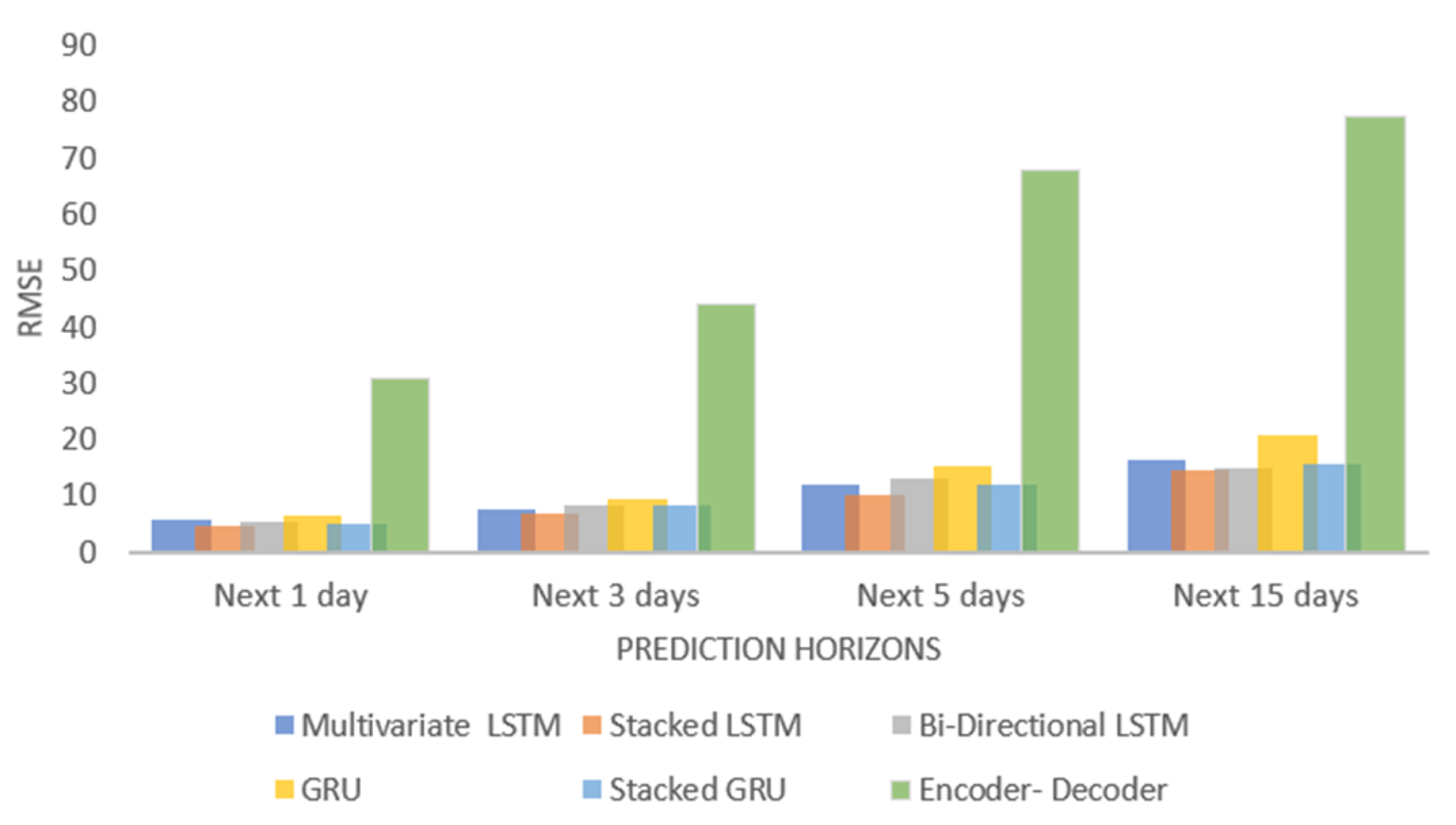
5.2. Comparison between Different Multivariate Models

This section examines the performance of six distinct multivariate models. The choice of these models is based on the result obtained from the univariate model analysis presented in Section 4.1. DL model (LSTM) outperforms the statistical (ARIMA) and ML (SVR) models. In Section 4.2, several multivariable models are explored to comprehend the effect of multivariable inputs on the DL (LSTM) model. In this part, several kinds of multivariate LSTM models are analyzed, and model accuracy is compared based on the RMSE error. The findings indicate that, out of six distinct kinds of LSTM models, stacked LSTM performed the best (six models are Multivariate, bi-directional, GRU, stacked GRU, and Encoder-Decoder). The Encoder-Decoder model seems to exhibit the problem of overfitting. The situation of overfitting occurs when a model performs extraordinarily well on the dataset used to train it but badly on new/unseen data, hence precluding its relevance. Overfitting is predominant when the model trains for too long (many training iterations) on a sample dataset and attempts to replicate irrelevant data details, including noise, resulting in poor generalization and a complicated model. Also, when there are insufficient data points, the model attempts to reproduce every single training data point and fails to discern relevant information in the data, leading to overfitting circumstances. The performance of the other five models, except for the Encoder-Decoder LSTM model, was superior to that of the univariate model. Among all models, the stacked LSTM performed the best with an RMSE of 14 when predicting the next 15 days of solar power generation at a case study site. The RMSE value for all tested multivariate models is presented in Figure 17 and Figure 18.

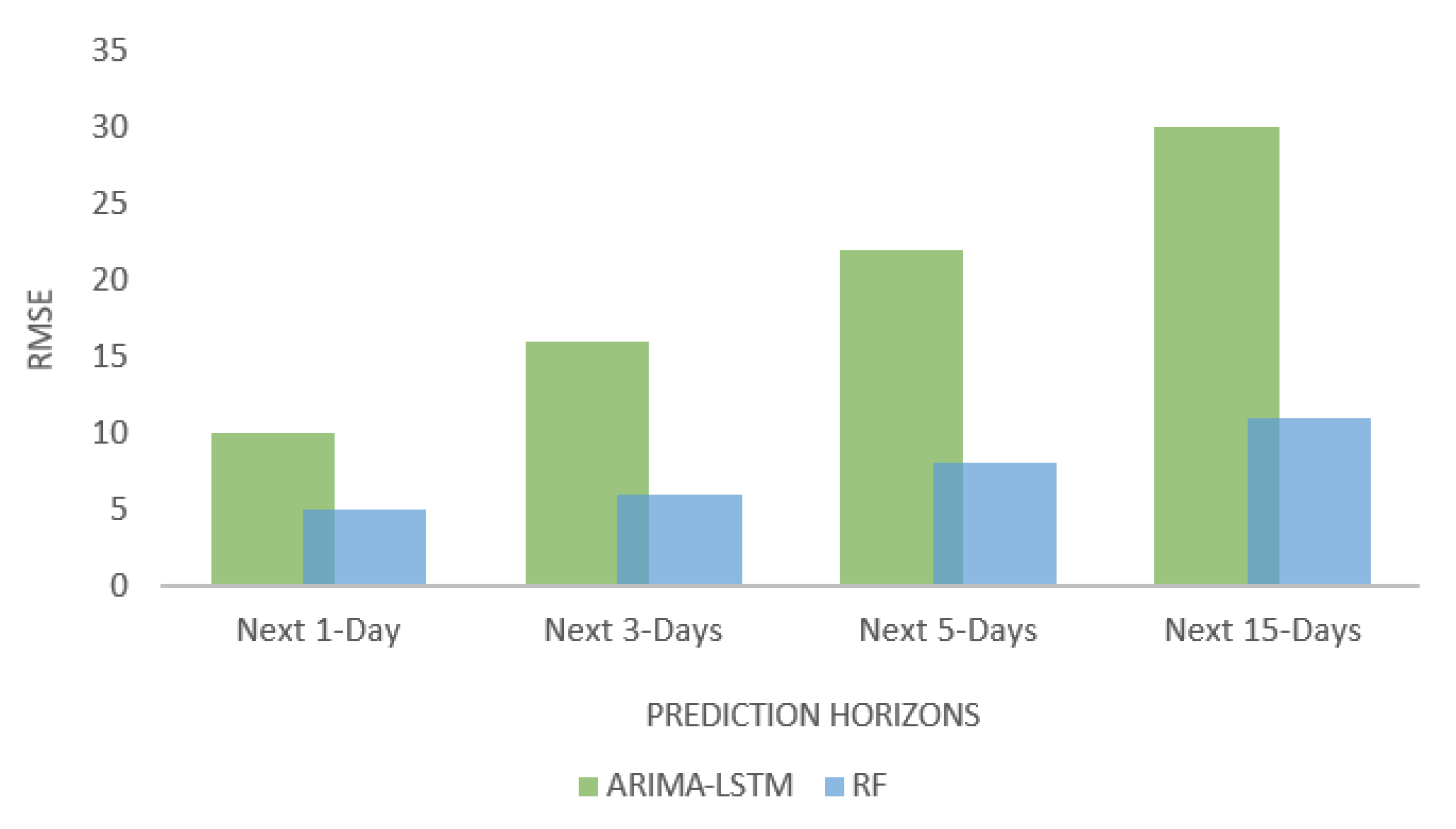
5.3. Comparison of Different Ensemble Models

The results suggest that the random forest ensemble model outperformed the ARIMA-LSTM hybrid model. The RF model predicted the next 360 h/15 days of solar power production with an RMSE value of 11. The hybrid ARIMA-LSTM model predicted the same with RMSE of 30. The hybrid ARIMA-LSTM model performed better than the ARIMA model alone but did not perform as well as the LSTM model alone. Figure 19 represents the RMSE value for different forecasting time horizons for the above two hybrid models. RF model outperformed all other 10 different univariate and multivariate statistical, ML, DL, and ensemble models. The best-performing ensemble model RF, actual versus predicted value for the next 15 days is presented in Figure 20.
In addition to the RMSE value comparison of different forecasting models, MAPE (Mean Absolute Percentage Error) value is also provided in the following Table 1.
M A P E = 1 n t = 1 n x j y j p x j × 100 %
Here, x j , y j p , and x j indicate the actual, predicted, and mean values of the solar power, respectively, and n is the number of samples. The limitation of the MAPE calculation is that the 0 value of actual solar power production should be disregarded. The abbreviations used in the table below- u, m, s, ED, b, t are univariate, multivariate, stacked, Encoder-Decoder, bidirectional, and prediction horizons, respectively.

6. Discussion

The study compares the effectiveness of four types of models: Statistical, Machine Learning (ML), Deep Learning (DL), and ensemble models, for forecasting solar power output over long terms using a case study of a hypothetical solar power plant located in Lubbock, Texas. The study found that the ML and DL models performed similarly and outperformed the statistical model. The statistical model was found to be unable to learn the intermittent nature of solar power production, thus it is not recommended for long-term forecasting of solar power generation.
The study further concludes that by adding five input variables (DNI, DHI, GHI, temperature, and wind speed), the ML and DL models improved their accuracy over univariate models (which use power output as the only input variable) by 36%. The study also found that while a slight increase in the prediction horizon caused the accuracy of the statistical model to decline drastically, a slight increase in the prediction horizon in the ML and DL models resulted in a gradual decrease in prediction accuracy.
Additionally, the study found that there was evidence of overfitting in a DL model (Encoder-Decoder) for small and univariate datasets whereas underfitting was observed in statistical and ML models when dealing with large and multivariate datasets. The Random Forest (RF) model was found to be the best-performing model among the four types of models tested, with 50% better accuracy over univariate models and 10% better accuracy over multivariate models. Therefore, the RF model is recommended for the case study’s setting.
The study suggests that future research could examine how the error distribution changes as the prediction horizon lengthens, which would be useful for estimating the confidence interval and ultimately for establishing the probabilistic character of forecasts. Similarly, it could be interesting to investigate the impact of adding feature engineering (the process of generating new features from pre-existing datasets) to ML/DL models.

7. Conclusions

In summary, the study provides a comprehensive performance analysis of various Statistical, ML, DL, and ensemble models for long-term forecasting of solar power output. The study found that the Random Forest (RF) model was the best-performing model among the four types of models tested, with 50% better accuracy over univariate models and 10% better accuracy over multivariate models. Thus, it is recommended for forecasting solar power output. This study is important for the renewable energy industry as accurate forecasting of solar power output is crucial for efficient planning and management of solar power plants. By understanding the strengths and limitations of different models, the industry can make informed decisions on which model to use for long-term solar power forecasting provided with the limited datasets and input variables. The future potential of this research is to apply these findings to real-world solar power plants and to continue to improve the accuracy of forecasting methods, which will play a key role in the sustainable development of renewable energy.

Author Contributions

Conceptualization, A.S. and S.P.; methodology, A.W.; software, S.G.; validation, Q.W., A.B. and A.D.; formal analysis, R.D.; investigation, A.S.; resources, S.P.; data curation, A.S.; writing—original draft preparation, S.P.; writing—review and editing, R.D.; visualization, S.P.; supervision, S.P.; project administration, S.P.; funding acquisition, S.P. All authors have read and agreed to the published version of the manuscript.

Funding

This research received no external funding.

Institutional Review Board Statement

Not Applicable.

Informed Consent Statement

Not Applicable.

Data Availability Statement

The data are available on request.

Acknowledgments

The authors would like to acknowledge Texas Tech University for providing the platform for the study.

Conflicts of Interest

The authors declare no conflict of interest.

References

  1. Dhakal, R.; Sedai, A.; Pol, S.; Parameswaran, S.; Nejat, A.; Moussa, H. A Novel Hybrid Method for Short-Term Wind Speed Prediction Based on Wind Probability Distribution Function and Machine Learning Models. Appl. Sci. 2022, 12, 9038. [Google Scholar] [CrossRef]
  2. Pol, S.; Houchens, B.; Marian, D.; Westergaard, C. Performance of AeroMINEs for Distributed Wind Energy. In Proceedings of the AIAA Scitech 2020 Forum, Orlando, FL, USA, 6–10 January 2020; p. 1241. [Google Scholar]
  3. Dhakal, R.; Yosfovand, M.; Prasai, S.; Sedai, A.; Pol, S.; Parameswaran, S.; Moussa, H. Deep Learning Model with Probability Density Function and Feature Engineering for Short Term Wind Speed Prediction. In Proceedings of the 2022 North American Power Symposium (NAPS), Salt Lake City, UT, USA, 9–11 October 2022; IEEE: New York, NY, USA, 2022; pp. 1–6. [Google Scholar]
  4. Natarajan, V.; Karatampati, P. Survey on renewable energy forecasting using different techniques. In Proceedings of the 2019 2nd International Conference on Power and Embedded Drive Control (ICPEDC), Chennai, India, 21–23 August 2019; IEEE: New York, NY, USA, 2019; pp. 349–354. [Google Scholar]
  5. Zaouali, K.; Rekik, R.; Bouallegue, R. Deep learning forecasting based on auto-lstm model for home solar power systems. In Proceedings of the 2018 IEEE 20th International Conference on High Performance Computing and Communications; IEEE 16th International Conference on Smart City; IEEE 4th International Conference on Data Science and Systems (Hpcc/Smartcity/Dss), Exeter, UK, 28–30 June 2018; IEEE: New York, NY, USA, 2018; pp. 235–242. [Google Scholar]
  6. Samanta, M.; Srikanth, B.; Yerrapragada, J.B. Short-Term Power Forecasting of Solar PV Systems Using Machine Learning Techniques. Environ. Sci. Comput. Sci. 2014, 2014, 18566286. [Google Scholar]
  7. Ahn, H.K.; Park, N. Deep RNN-based photovoltaic power short-term forecast using power IoT sensors. Energies 2021, 14, 436. [Google Scholar] [CrossRef]
  8. Harrou, F.; Kadri, F.; Sun, Y. Forecasting of photovoltaic solar power production using LSTM approach. Adv. Stat. Model. Forecast. Fault Detect. Renew. Energy Syst. 2020, 3. [Google Scholar]
  9. Gao, M.; Li, J.; Hong, F.; Long, D. Day-ahead power forecasting in a large-scale photovoltaic plant based on weather classification using LSTM. Energy 2019, 187, 115838. [Google Scholar] [CrossRef]
  10. Sharma, J.; Soni, S.; Paliwal, P.; Saboor, S.; Chaurasiya, P.K.; Sharifpur, M. A novel long term solar photovoltaic power forecasting approach using LSTM with Nadam optimizer: A case study of India. Energy Sci. Eng. 2022, 10, 2909–2929. [Google Scholar] [CrossRef]
  11. Fara, L.; Diaconu, A.; Craciunescu, D.; Fara, S. Forecasting of Energy Production for Photovoltaic Systems Based on ARIMA and ANN Advanced Models. Int. J. Photoenergy 2021, 2021, 6777488. [Google Scholar] [CrossRef]
  12. Sengupta, M.; Habte, A.; Wilbert, S.; Gueymard, C.; Remund, J. Best Practices Handbook for the Collection and Use of Solar Resource Data for Solar Energy Applications; National Renewable Energy Lab.(NREL): Golden, CO, USA, 2021. [Google Scholar]
  13. Sobri, S.; Koohi-Kamali, S.; Rahim, N.A. Solar photovoltaic generation forecasting methods: A review. Energy Convers. Manag. 2018, 156, 459–497. [Google Scholar] [CrossRef]
  14. Morf, H. Sunshine and cloud cover prediction based on Markov processes. Sol. Energy 2014, 110, 615–626. [Google Scholar] [CrossRef]
  15. Fan, J.; Wu, L.; Zhang, F.; Cai, H.; Zeng, W.; Wang, X.; Zou, H. Empirical and machine learning models for predicting daily global solar radiation from sunshine duration: A review and case study in China. Renew. Sustain. Energy Rev. 2019, 100, 186–212. [Google Scholar] [CrossRef]
  16. Wahab, M.A. New approach to estimate Ångström coefficients. Sol. Energy 1993, 51, 241–245. [Google Scholar] [CrossRef]
  17. Kumler, A.; Xie, Y.; Zhang, Y. A New Approach for Short-Term Solar Radiation Forecasting Using the Estimation of Cloud Fraction and Cloud Albedo; National Renewable Energy Lab.(NREL): Golden, CO, USA, 2018. [Google Scholar]
  18. Akinoǧlu, B. A review of sunshine-based models used to estimate monthly average global solar radiation. Renew. Energy 1991, 1, 479–497. [Google Scholar] [CrossRef]
  19. Fan, J.; Wang, X.; Zhang, F.; Ma, X.; Wu, L. Predicting daily diffuse horizontal solar radiation in various climatic regions of China using support vector machine and tree-based soft computing models with local and extrinsic climatic data. J. Clean. Prod. 2020, 248, 119264. [Google Scholar] [CrossRef]
  20. Tuohy, A.; Zack, J.; Haupt, S.E.; Sharp, J.; Ahlstrom, M.; Dise, S. Solar forecasting: Methods, challenges, and performance. IEEE Power Energy Mag. 2015, 13, 50–59. [Google Scholar] [CrossRef]
  21. Choudhary, A.; Pandey, D.; Kumar, A. A review of various techniques for solar radiation estimation, In Proceedings of the 2019 3rd International Conference on Recent Developments in Control, Automation & Power Engineering (RDCAPE), Noida, India, 10–11 October 2019; IEEE: New York, NY, USA, 2019; pp. 169–174. [Google Scholar]
  22. Dazhi, Y.; Walsh, W.; Zibo, D.; Jirutitijaroen, P.; Reindl, T.G. Block matching algorithms: Their applications and limitations in solar irradiance forecasting. Energy Procedia 2013, 33, 335–342. [Google Scholar] [CrossRef] [Green Version]
  23. Gürel, A.E.; Ağbulut, Ü.; Biçen, Y. Assessment of machine learning, time series, response surface methodology and empirical models in prediction of global solar radiation. J. Clean. Prod. 2020, 277, 122353. [Google Scholar] [CrossRef]
  24. Wang, K.; Qi, X.; Liu, H. A comparison of day-ahead photovoltaic power forecasting models based on deep learning neural network. Appl. Energy 2019, 251, 113315. [Google Scholar] [CrossRef]
  25. Wang, H.; Lei, Z.; Zhang, X.; Zhou, B.; Peng, J. A review of deep learning for renewable energy forecasting. Energy Convers. Manag. 2019, 198, 111799. [Google Scholar] [CrossRef]
  26. Li, P.; Zhou, K.; Lu, X.; Yang, S. A hybrid deep learning model for short-term PV power forecasting. Appl. Energy 2020, 259, 114216. [Google Scholar] [CrossRef]
  27. Habte, A.; Sengupta, M.; Lopez, A. Evaluation of the National Solar Radiation Database (NSRDB): 1998–2015; National Renewable Energy Lab.(NREL): Golden, CO, USA, 2017. [Google Scholar]
  28. Freeman, J.M.; DiOrio, N.A.; Blair, N.J.; Neises, T.W.; Wagner, M.J.; Gilman, P.; Janzou, S. System Advisor Model (SAM) General Description (Version 2017.9. 5); National Renewable Energy Lab.(NREL): Golden, CO, USA, 2018. [Google Scholar]
  29. Bisong, E. Matplotlib and seaborn. In Building Machine Learning and Deep Learning Models on Google Cloud platform; Springer: Berlin/Heidelberg, Germany, 2019; pp. 151–165. [Google Scholar]
  30. Faber, N.K.M. Estimating the uncertainty in estimates of root mean square error of prediction: Application to determining the size of an adequate test set in multivariate calibration. Chemom. Intell. Lab. Syst. 1999, 49, 79–89. [Google Scholar] [CrossRef]
  31. Hillmer, S.C.; Tiao, G.C. An ARIMA-model-based approach to seasonal adjustment. J. Am. Stat. Assoc. 1982, 77, 63–70. [Google Scholar] [CrossRef]
  32. Newbold, P. ARIMA model building and the time series analysis approach to forecasting. J. Forecast. 1983, 2, 23–35. [Google Scholar] [CrossRef]
  33. Noureen, S.; Atique, S.; Roy, V.; Bayne, S. Analysis and application of seasonal ARIMA model in Energy Demand Forecasting: A case study of small scale agricultural load. In Proceedings of the 2019 IEEE 62nd International Midwest Symposium on Circuits and Systems (MWSCAS), Dallas, TX, USA, 4–7 August 2019; IEEE: New York, NY, USA, 2019; pp. 521–524. [Google Scholar]
  34. Burnham, K.P.; Anderson, D.R. Multimodel inference: Understanding AIC and BIC in model selection. Sociol. Methods Res. 2004, 33, 261–304. [Google Scholar] [CrossRef]
  35. Ibrahim, I.; Abdulazeez, A. The role of machine learning algorithms for diagnosing diseases. J. Appl. Sci. Technol. Trends 2021, 2, 10–19. [Google Scholar] [CrossRef]
  36. Behravan, I.; Razavi, S.M. A novel machine learning method for estimating football players’ value in the transfer market. Soft Comput. 2021, 25, 2499–2511. [Google Scholar] [CrossRef]
  37. Zhou, D.-X.; Jetter, K. Approximation with polynomial kernels and SVM classifiers. Adv. Comput. Math. 2006, 25, 323–344. [Google Scholar] [CrossRef]
  38. Gopi, A.P.; Jyothi, R.; Narayana, V.; Sandeep, K.S. Classification of tweets data based on polarity using improved RBF kernel of SVM. Int. J. Inf. Technol. 2020, 1–16. [Google Scholar] [CrossRef]
  39. Wang, J.; Chen, Q.; Chen, Y. RBF kernel based support vector machine with universal approximation and its application. In International Symposium on Neural Networks; Springer: Berlin/Heidelberg, Germany, 2004; pp. 512–517. [Google Scholar]
  40. Huang, Q.; Mao, J.; Liu, Y. An improved grid search algorithm of SVR parameters optimization. In Proceedings of the 2012 IEEE 14th International Conference on Communication Technology, Chengdu, China, 9–11 November 2012; IEEE: New York, NY, USA, 2012; pp. 1022–1026. [Google Scholar]
  41. Xue, H.; Huynh, D.; Reynolds, M. SS-LSTM: A hierarchical LSTM model for pedestrian trajectory prediction. In Proceedings of the 2018 IEEE Winter Conference on Applications of Computer Vision (WACV), Lake Tahoe, NV, USA, 12–15 March 2018; IEEE: New York, NY, USA, 2018; pp. 1186–1194. [Google Scholar]
  42. Liu, Y.; Sun, C.; Lin, L.; Wang, X. Learning natural language inference using bidirectional LSTM model and inner-attention. arXiv Prepr. 2016, arXiv:1605.09090. [Google Scholar]
  43. Khatiwada, A.; Kadariya, P.; Agrahari, S.; Dhakal, R. Big Data Analytics and Deep Learning Based Sentiment Analysis System for Sales Prediction. In Proceedings of the 2019 IEEE Pune Section International Conference (PuneCon), Pune, India, 18–20 December 2019; IEEE: New York, NY, USA, 2019; pp. 1–6. [Google Scholar]
  44. Yao, K.; Cohn, T.; Vylomova, K.; Duh, K.; Dyer, C. Depth-gated LSTM. arXiv 2015, arXiv:1508.03790. [Google Scholar]
  45. Randles, B.M.; Pasquetto, I.; Golshan, M.; Borgman, C.L. Using the Jupyter notebook as a tool for open science: An empirical study. In Proceedings of the 2017 ACM/IEEE Joint Conference on Digital Libraries (JCDL), Toronto, ON, Canada, 19–23 June 2017; IEEE: New York, NY, USA, 2017; pp. 1–2. [Google Scholar]
  46. Sundermeyer, M.; Schlüter, R.; Ney, H. LSTM neural networks for language modeling. In Proceedings of the Thirteenth Annual Conference of the International Speech Communication Association, Portland, OR, USA, 9–13 September 2012. [Google Scholar]
  47. Chandriah, K.K.; Naraganahalli, R.V. RNN/LSTM with modified Adam optimizer in deep learning approach for automobile spare parts demand forecasting. Multimed. Tools Appl. 2021, 80, 26145–26159. [Google Scholar] [CrossRef]
  48. Yu, L.; Qu, J.; Gao, F.; Tian, Y. A novel hierarchical algorithm for bearing fault diagnosis based on stacked LSTM. Shock. Vib. 2019, 2019, 2756284. [Google Scholar] [CrossRef]
  49. Zhao, R.; Yan, R.; Wang, J.; Mao, K. Learning to monitor machine health with convolutional bi-directional LSTM networks. Sensors 2017, 17, 273. [Google Scholar] [CrossRef] [Green Version]
  50. Malhotra, P.; Ramakrishnan, A.; Anand, G.; Vig, L.; Agarwal, P.; Shroff, G. LSTM-based encoder-decoder for multi-sensor anomaly detection. arXiv 2016, arXiv:1607.00148. [Google Scholar]
  51. Pavithra, M.; Saruladha, K.; Sathyabama, K. GRU based deep learning model for prognosis prediction of disease progression. In Proceedings of the 2019 3rd International Conference on Computing Methodologies and Communication (ICCMC), Tamil Nadu, India, 27–29 March 2019; IEEE: New York, NY, USA, 2019; pp. 840–844. [Google Scholar]
  52. Dey, R.; Salem, F.M. Gate-variants of gated recurrent unit (GRU) neural networks. In Proceedings of the 2017 IEEE 60th International Midwest Symposium on Circuits and Systems (MWSCAS), Boston, MA, USA, 6–9 August 2017; IEEE: New York, NY, USA, 2017; pp. 1597–1600. [Google Scholar]
  53. Sun, P.; Boukerche, A.; Tao, Y. SSGRU: A novel hybrid stacked GRU-based traffic volume prediction approach in a road network. Comput. Commun. 2020, 160, 502–511. [Google Scholar] [CrossRef]
  54. Leutbecher, M.; Palmer, T.N. Ensemble forecasting. J. Comput. Phys. 2008, 227, 3515–3539. [Google Scholar] [CrossRef]
  55. Moon, J.; Kim, Y.; Son, M.; Hwang, E. Hybrid short-term load forecasting scheme using random forest and multilayer perceptron. Energies 2018, 11, 3283. [Google Scholar] [CrossRef] [Green Version]
  56. Bordarie, J. Predicting intentions to comply with speed limits using a ‘decision tree’ applied to an extended version of the theory of planned behaviour. Transp. Res. Part F Traffic Psychol. Behav. 2019, 63, 174–185. [Google Scholar] [CrossRef]
  57. Kumar, M.; Thenmozhi, M. Forecasting stock index movement: A comparison of support vector machines and random forest. In Indian Institute of Capital Markets 9th Capital Markets Conference Paper; Indian Institute of Capital Markets: Navi Mumbai, India, 2006. [Google Scholar]
  58. Andrews, B.H.; Dean, M.; Swain, R.; Cole, C. Building ARIMA and ARIMAX models for predicting long-term disability benefit application rates in the public/private sectors. Soc. Actuar. 2013, 1–54. [Google Scholar]
  59. Hashemi, R.; Brigode, P.; Garambois, P.-A.; Javelle, P. How can we benefit from regime information to make more effective use of long short-term memory (LSTM) runoff models? Hydrol. Earth Syst. Sci. 2022, 26, 5793–5816. [Google Scholar] [CrossRef]
  60. Choi, H.K. Stock price correlation coefficient prediction with ARIMA-LSTM hybrid model. ArXiv 2018, arXiv:1808.01560. [Google Scholar]
  61. Fathi, O. Time series forecasting using a hybrid ARIMA and LSTM model. Velv. Consult. 2019, 1–7. [Google Scholar]
Figure 1. Methodology of the study.
Forecasting 05 00014 g001
Figure 2. Input variables and models used in the study.
Forecasting 05 00014 g002
Figure 3. Graphical representation of data utilized in the study.
Forecasting 05 00014 g003
Figure 4. Methodology of forecasting using ARIMA mode.
Forecasting 05 00014 g004
Figure 5. ACF and PACF plot.
Forecasting 05 00014 g005
Figure 6. Basic structure of SVR model.
Forecasting 05 00014 g006
Figure 7. Basic architecture of LSTM model.
Forecasting 05 00014 g007
Figure 8. Basic architecture of Multivariate LSTM model.
Forecasting 05 00014 g008
Figure 9. Basic architecture of the stacked LSTM model.
Forecasting 05 00014 g009
Figure 10. Basic architecture of the Bi-Directional LSTM model.
Forecasting 05 00014 g010
Figure 11. Basic architecture of the Encoder-Decoder LSTM model.4.2.5. GRU.
Forecasting 05 00014 g011
Figure 12. Basic structure of the GRU model.
Forecasting 05 00014 g012
Figure 13. Basic architecture of stacked GRU model.
Forecasting 05 00014 g013
Figure 14. Basic architecture of the Random Forest (RF) model [17,57].
Forecasting 05 00014 g014
Figure 15. Comparison between the ARIMA, SVR, and LSTM model for solar power forecasting. Row 1, 2, 3 and 4 represents comparison between models for next 1-day, 3-days, 5-days and 15-days prediction respectively. Column 1, 2, 3 represents ARIMA, SVR and LSTM model respectively (red line = actual, blue line = Predicted).
Forecasting 05 00014 g015
Figure 16. Comparison between ARIMA, SVR, and LSTM models.
Forecasting 05 00014 g016
Figure 17. Comparision between several multivariate models.
Forecasting 05 00014 g017
Figure 18. Performance of the Stacked LSTM model for predicting 15 days-ahead solar power generation (red line = actual value, blue line = predicted value).
Forecasting 05 00014 g018
Figure 19. Comparison of the performance of ensemble models.
Forecasting 05 00014 g019
Figure 20. Peformance of the RF model for predicting next 15 days-ahead solar power generation (red line = actual value, blue line = predicted value).
Forecasting 05 00014 g020
Table 1. Performance results of different forecasting models.
Modelt = 1 Dayt = 3 Dayst = 5 Dayst = 15 Days
ARIMA0.420.81.362.24
SVR0.070.110.160.34
u-LSTM0.080.120.190.28
m-LSTM0.060.100.120.18
s-LSTM0.050.080.110.16
GRU0.070.100.130.20
s-GRU0.060.100.120.17
ED-LSTM1.972.012.122.13
b-LSTM0.090.130.150.19
ARIMA-LSTM0.120.170.200.25
RF0.030.070.100.13
Disclaimer/Publisher’s Note: The statements, opinions and data contained in all publications are solely those of the individual author(s) and contributor(s) and not of MDPI and/or the editor(s). MDPI and/or the editor(s) disclaim responsibility for any injury to people or property resulting from any ideas, methods, instructions or products referred to in the content.

