
Coupling a Neural Network with a Spatial Downscaling Procedure to Improve Probabilistic Nowcast for Urban Rain Radars


Abstract
:1. Introduction
2. Materials and Methods
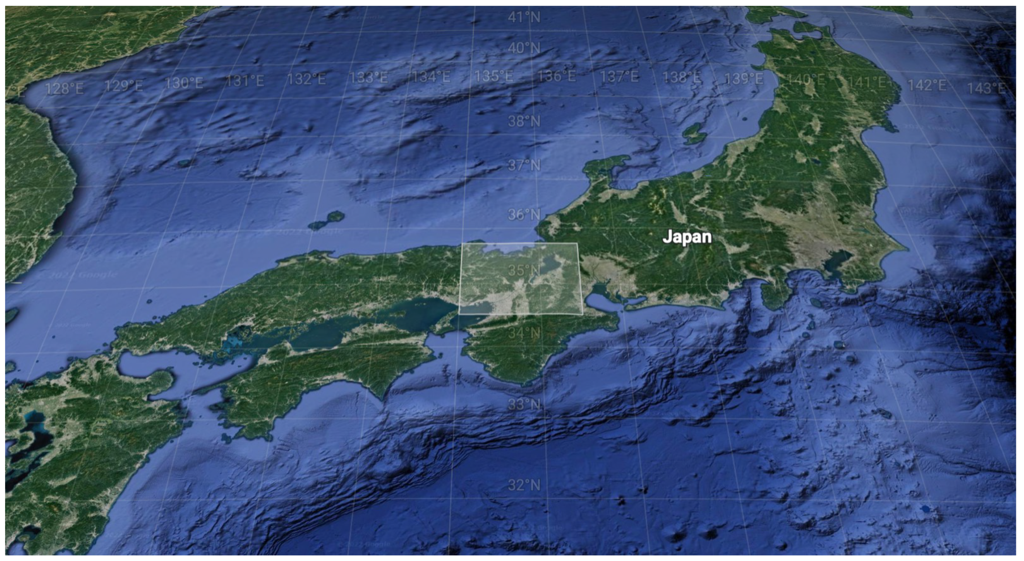
2.1. Data
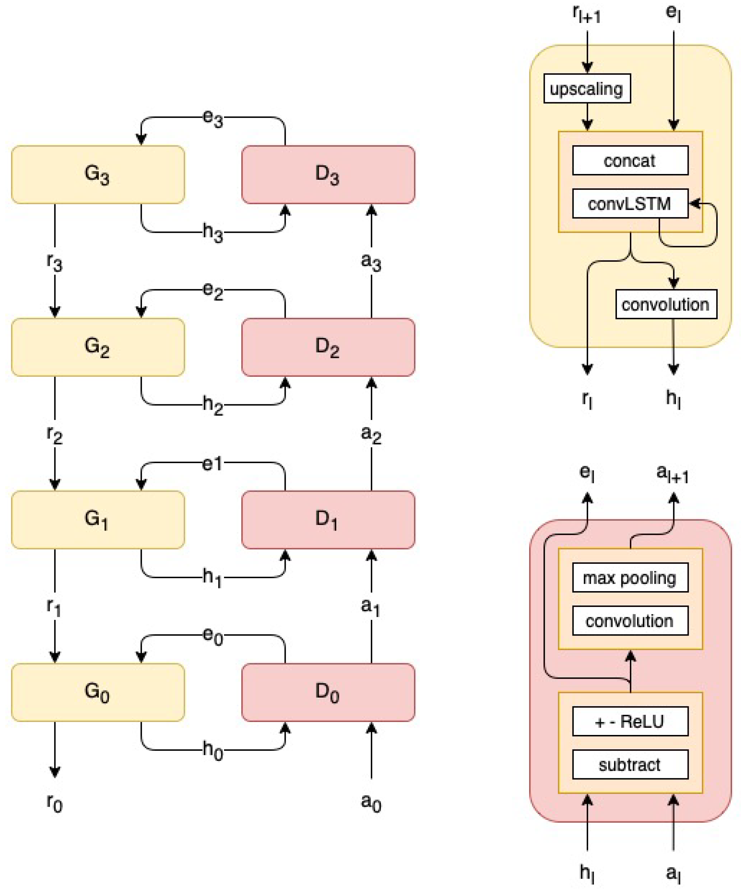
2.2. PredNet
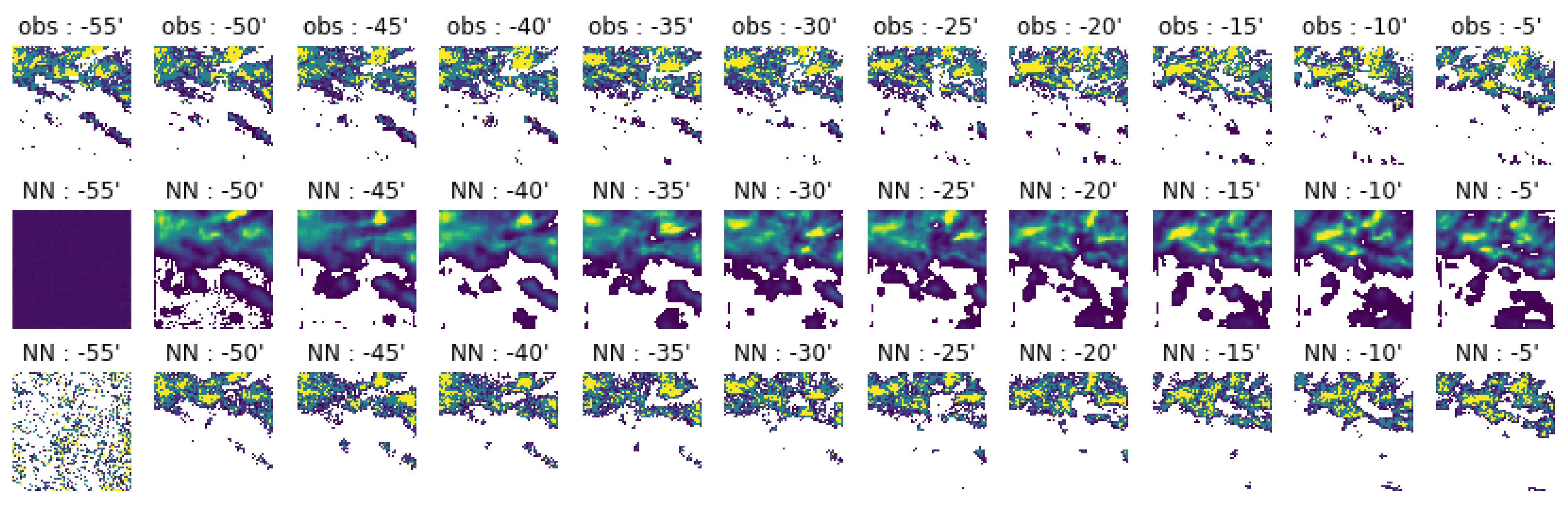
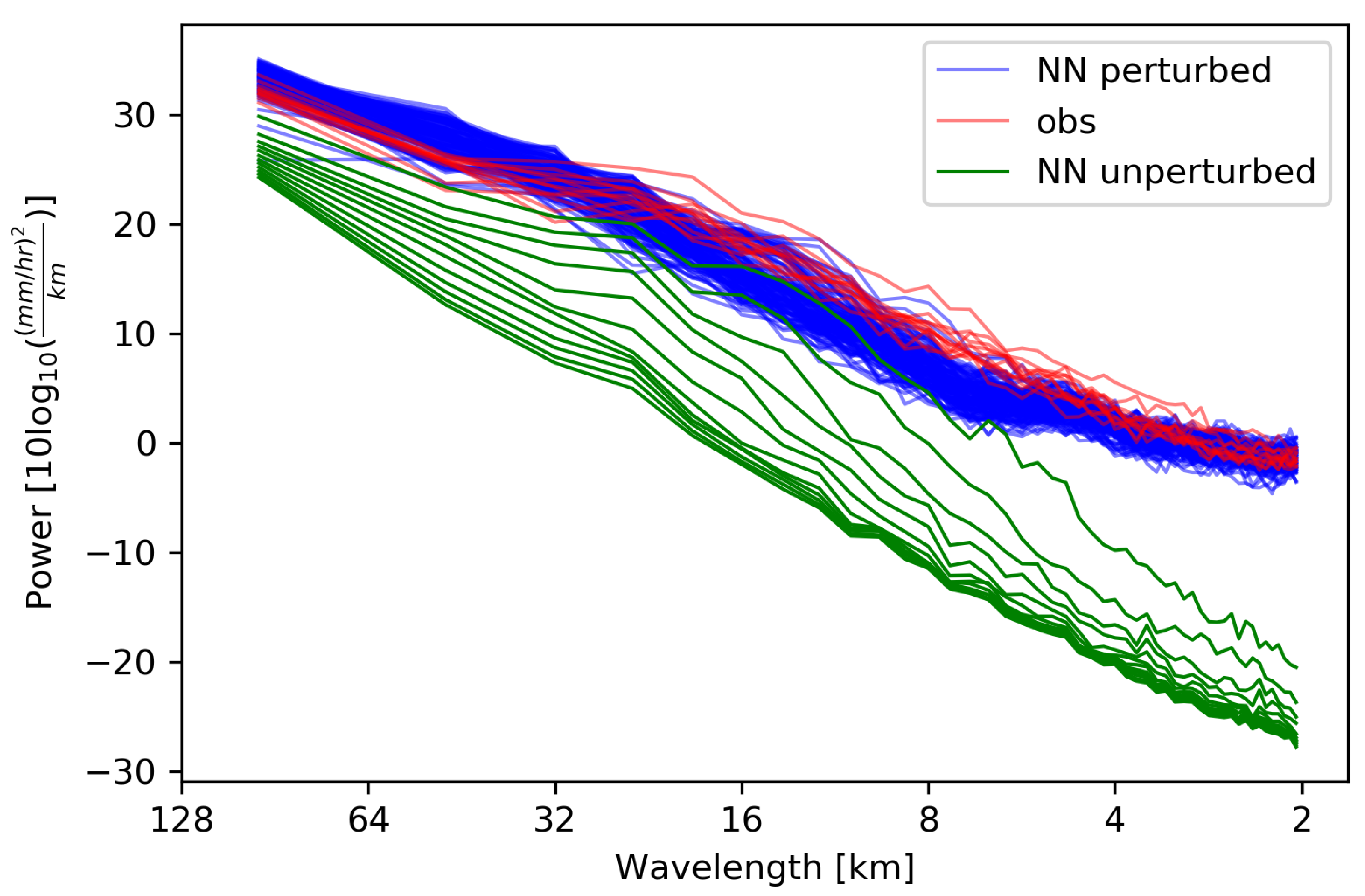
2.3. Proposed Methodology: Stochastic PredNet
- A set of equally probable scenarios S is generated in the hour before the forecast is issued, injecting into the neural network’s estimate D of the measured data a noise component consistent with the difference in spatial detail between the measured data and those “assimilated” by the network itself, using the multipliers N defined in Equation (5);
- With the same method, at each nowcast time step f ahead of 5’, a stochastic component, consistent with the uncertainty evaluated under similar conditions in the period immediately preceding its emission, is added to the prediction;
- We impose that the mean value of the ensemble members is equal to the deterministic unperturbed prediction of PredNet ( precedure), and that the Cumulative Distribution Function ( precedure) of the predicted field is equal to that of the last observed field;
- Starting from step 2, the procedure is iterated for all 12 time steps of 5’ each, and for each ensemble member, obtaining , the one-hour forecast for the chosen number M of scenarios.
| Algorithm 1: Pseudocode of the stochastic PredNet algorithm |
 |
2.4. The Benchmark Nowcast Technique: STEPS
3. Results
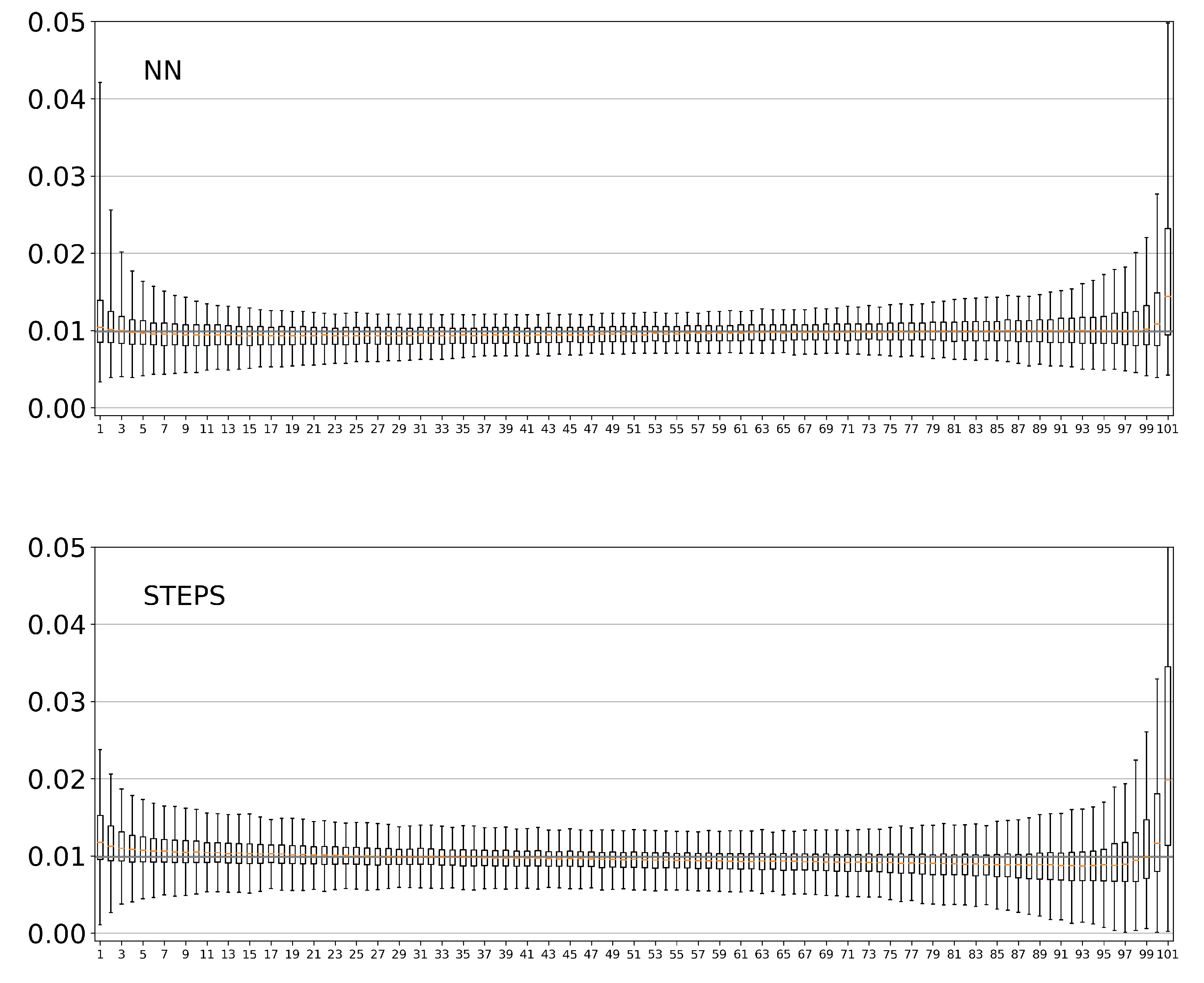
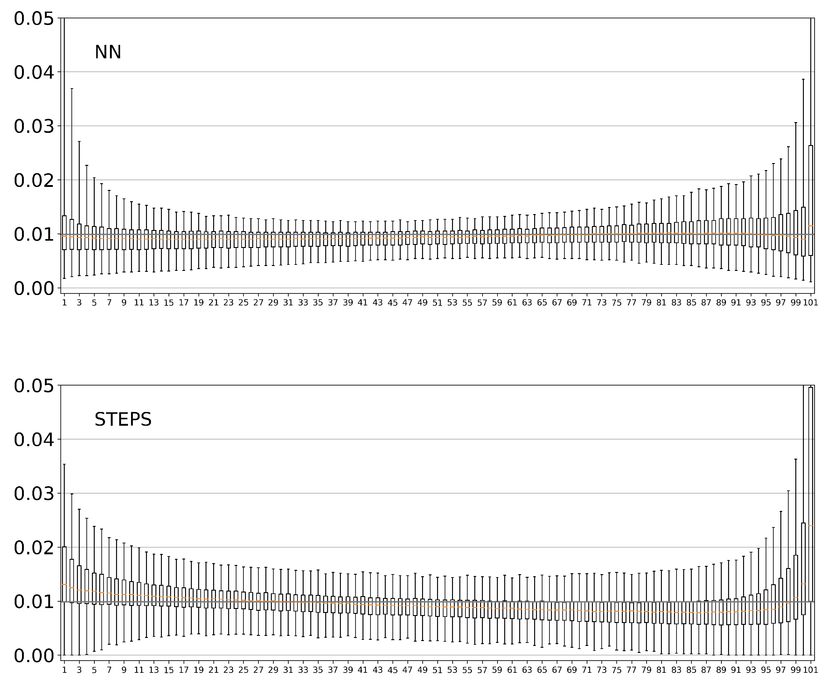
3.1. Spread–Skill
3.2. CRPS
3.3. Rank Histogram
3.4. Reliability Diagram
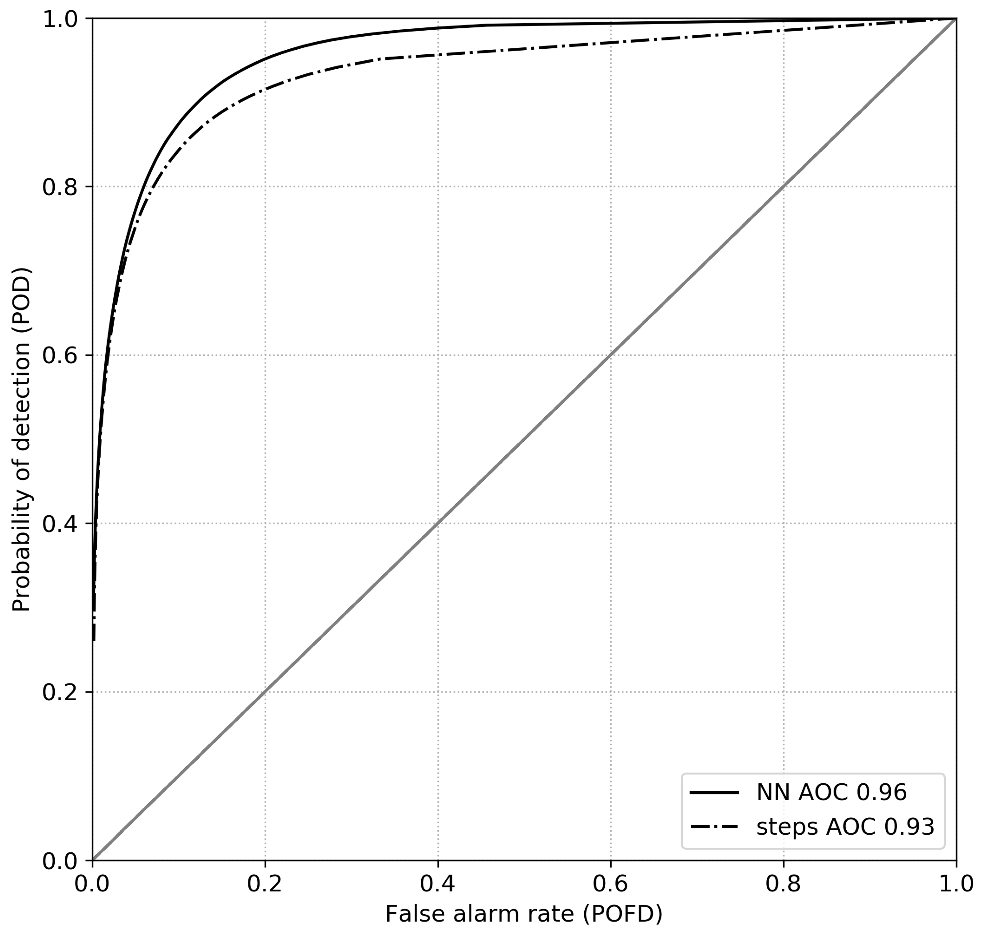
3.5. ROC Curve
4. Discussion
- We proposed a physical-statistical interpretation of the result obtained from the application of the PredNet network for the nowcasting of radar images, as the ensemble mean of a probabilistic forecast;
- This interpretation was tested by constructing around the unperturbed forecast an ensemble of scenarios obtained by adding noise, with the correct spatial correlation, compatible with the scales not explicitly resolved by the PredNet;
- The detailed analysis made on extended data set leads us to conclude that the method we proposed has performance superior or equal to the probabilistic STEPS method, which represents a well recognized benchmark;
- The proposed solution, based on a generative model, succeeds at providing an overall good quality probabilistic prediction for the entire domain covered by the radar and thus solves the problem that occurs when implementing a prediction procedure based on optical flow for a radar of limited spatial range;
- For a domain of small size, the extrapolation phase of the procedure can be performed with limited computational resources, allowing it to be performed in low-cost edge-computing devices that can be included in the same radar apparatus.
Author Contributions
Funding
Institutional Review Board Statement
Informed Consent Statement
Data Availability Statement
Conflicts of Interest
References
- Schmid, F.; Wang, Y.; Harou, A. Nowcasting Guidelines—A Summary. Bull. N° 2019, 68, 2. [Google Scholar]
- Ayzel, G.; Heistermann, M.; Winterrath, T. Optical flow models as an open benchmark for radar-based precipitation nowcasting (rainymotion v0. 1). Geosci. Model Dev. 2019, 12, 1387–1402. [Google Scholar] [CrossRef] [Green Version]
- Dixon, M.; Wiener, G. TITAN: Thunderstorm identification, tracking, analysis, and nowcasting—A radar-based methodology. J. Atmos. Ocean. Technol. 1993, 10, 785–797. [Google Scholar] [CrossRef]
- Chang, P.L.; Zhang, J.; Tang, Y.S.; Tang, L.; Lin, P.F.; Langston, C.; Kaney, B.; Chen, C.R.; Howard, K. An operational multi-radar multi-sensor QPE system in Taiwan. Bull. Am. Meteorol. Soc. 2021, 102, E555–E577. [Google Scholar] [CrossRef]
- Smith, K.; Austin, G. Nowcasting precipitation—A proposal for a way forward. J. Hydrol. 2000, 239, 34–45. [Google Scholar] [CrossRef]
- Chung, K.S.; Yao, I.A. Improving radar echo Lagrangian extrapolation nowcasting by blending numerical model wind information: Statistical performance of 16 typhoon cases. Mon. Weather Rev. 2020, 148, 1099–1120. [Google Scholar] [CrossRef]
- Radhakrishnan, C.; Chandrasekar, V. CASA prediction system over dallas–fort worth urban network: Blending of nowcasting and high-resolution numerical weather prediction model. J. Atmos. Ocean. Technol. 2020, 37, 211–228. [Google Scholar] [CrossRef]
- Bowler, N.E.; Pierce, C.E.; Seed, A.W. STEPS: A probabilistic precipitation forecasting scheme which merges an extrapolation nowcast with downscaled NWP. Q. J. R. Meteorol. Soc. 2006, 132, 2127–2155. [Google Scholar] [CrossRef]
- Seed, A. A dynamic and spatial scaling approach to advection forecasting. J. Appl. Meteorol. 2003, 42, 381–388. [Google Scholar] [CrossRef]
- Velasco-Forero, C.; Pudashine, J.; Curtis, M.; Seed, A. STEPS3–ADV–VERIFICATION REPORT; National Library of Australia Cataloguing-in-Publication Entry: Melbourne, VIC, Australia, 2020. [Google Scholar] [CrossRef]
- Pulkkinen, S.; Chandrasekar, V.; Harri, A.M. Fully spectral method for radar-based precipitation nowcasting. IEEE J. Sel. Top. Appl. Earth Obs. Remote Sens. 2019, 12, 1369–1382. [Google Scholar] [CrossRef]
- Shi, X.; Chen, Z.; Wang, H.; Yeung, D.Y.; Wong, W.K.; Woo, W.c. Convolutional LSTM network: A machine learning approach for precipitation nowcasting. In Proceedings of the Advances in Neural Information Processing Systems, Montreal, QC, Canada, 7–12 December 2015; pp. 802–810. [Google Scholar]
- Shi, X.; Gao, Z.; Lausen, L.; Wang, H.; Yeung, D.Y.; Wong, W.K.; Woo, W.C. Deep learning for precipitation nowcasting: A benchmark and a new model. In Proceedings of the Advances in Neural Information Processing Systems, Long Beach, CA, USA, 4–9 December 2017; pp. 5617–5627. [Google Scholar]
- Ayzel, G.; Scheffer, T.; Heistermann, M. RainNet v1. 0: A convolutional neural network for radar-based precipitation nowcasting. Geosci. Model Dev. 2020, 13, 2631–2644. [Google Scholar] [CrossRef]
- Foresti, L.; Sideris, I.V.; Nerini, D.; Beusch, L.; Germann, U. Using a 10-year radar archive for nowcasting precipitation growth and decay: A probabilistic machine learning approach. Weather Forecast. 2019, 34, 1547–1569. [Google Scholar] [CrossRef]
- Trebing, K.; Stanczyk, T.; Mehrkanoon, S. SmaAt-UNet: Precipitation nowcasting using a small attention-UNet architecture. Pattern Recognit. Lett. 2021, 145, 178–186. [Google Scholar] [CrossRef]
- Sønderby, C.K.; Espeholt, L.; Heek, J.; Dehghani, M.; Oliver, A.; Salimans, T.; Agrawal, S.; Hickey, J.; Kalchbrenner, N. MetNet: A Neural Weather Model for Precipitation Forecasting. arXiv 2020, arXiv:2003.12140. [Google Scholar]
- Ravuri, S.; Lenc, K.; Willson, M.; Kangin, D.; Lam, R.; Mirowski, P.; Fitzsimons, M.; Athanassiadou, M.; Kashem, S.; Madge, S.; et al. Skilful precipitation nowcasting using deep generative models of radar. Nature 2021, 597, 672–677. [Google Scholar] [CrossRef] [PubMed]
- Bouget, V.; Béréziat, D.; Brajard, J.; Charantonis, A.; Filoche, A. Fusion of rain radar images and wind forecasts in a deep learning model applied to rain nowcasting. arXiv 2020, arXiv:2012.05015. [Google Scholar] [CrossRef]
- Ashesh, A.; Chang, C.T.; Chen, B.F.; Lin, H.T.; Chen, B.; Huang, T.S. Accurate and Clear Quantitative Precipitation Nowcasting Based on a Deep Learning Model with Consecutive Attention and Rain-Map Discrimination. Artif. Intell. Earth Syst. 2022, 1, e210005. [Google Scholar] [CrossRef]
- Lotter, W.; Kreiman, G.; Cox, D. Deep predictive coding networks for video prediction and unsupervised learning. arXiv 2016, arXiv:1605.08104. [Google Scholar]
- Marrocu, M.; Massidda, L. Performance comparison between deep learning and optical flow-based techniques for nowcast precipitation from radar images. Forecasting 2020, 2, 194–210. [Google Scholar] [CrossRef]
- Farris, S.; Seoni, A.; Ruggiu, D.; Bertoldo, S.; Perona, G.; Allegretti, M.; Marrocu, M.; Badas, M.; Viola, F.; Deidda, R. First analyses of rainfall patterns retrieved by a newly installed X-band radar over the Metropolitan area of Cagliari (Sardinia, Italy). In Rainfall Monitoring, Modelling and Forecasting in Urban Environment. UrbanRain18: 11th International Workshop on Precipitation in Urban Areas. Conference Proceedings; ETH Zurich, Institute of Environmental Engineering: Pontresina, Switzerland, 2019; pp. 39–40. [Google Scholar]
- Sato, R.; Kashima, H.; Yamamoto, T. Short-Term Precipitation Prediction with Skip-Connected PredNet. In Proceedings of the International Conference on Artificial Neural Networks, Rhodes, Greece, 4–7 October 2018; Springer: Berlin/Heidelberg, Germany, 2018; pp. 373–382. [Google Scholar]
- Van Rossum, G.; Drake, F.L. Python 3 Reference Manual; CreateSpace: Scotts Valley, CA, USA, 2009. [Google Scholar]
- Paszke, A.; Gross, S.; Massa, F.; Lerer, A.; Bradbury, J.; Chanan, G.; Killeen, T.; Lin, Z.; Gimelshein, N.; Antiga, L.; et al. PyTorch: An Imperative Style, High-Performance Deep Learning Library. In Advances in Neural Information Processing Systems 32; Wallach, H., Larochelle, H., Beygelzimer, A., d’Alché-Buc, F., Fox, E., Garnett, R., Eds.; Curran Associates, Inc.: Vancouver, BC, Canada, 2019; pp. 8024–8035. [Google Scholar]
- Rebora, N.; Ferraris, L.; Hardenberg, J.; Provenzale, A. RainFARM: Rainfall Downscaling by a Filtered Autoregressive Model. J. Hydrometeorol. 2006, 7, 724–738. [Google Scholar] [CrossRef]
- Pulkkinen, S.; Nerini, D.; Pérez Hortal, A.A.; Velasco-Forero, C.; Seed, A.; Germann, U.; Foresti, L. Pysteps: An open-source Python library for probabilistic precipitation nowcasting (v1. 0). Geosci. Model Dev. 2019, 12, 4185–4219. [Google Scholar] [CrossRef] [Green Version]
- Lucas, B.D.; Kanade, T. An iterative image registration technique with an application to stereo vision. In Proceedings of the Seventh International Joint Conference on Artificial Intelligence, Vancouver, BC, Canada, 24–28 August 1981; pp. 674–679. [Google Scholar]
- Bouguet, J.Y. Pyramidal implementation of the affine lucas kanade feature tracker description of the algorithm. Intel Corp. 2001, 5, 4. [Google Scholar]
- Laroche, S.; Zawadzki, I. Retrievals of horizontal winds from single-Doppler clear-air data by methods of cross correlation and variational analysis. J. Atmos. Ocean. Technol. 1995, 12, 721–738. [Google Scholar] [CrossRef]
- Germann, U.; Zawadzki, I. Scale-dependence of the predictability of precipitation from continental radar images. Part I: Description of the methodology. Mon. Weather Rev. 2002, 130, 2859–2873. [Google Scholar] [CrossRef]
- Ruzanski, E.; Chandrasekar, V.; Wang, Y. The CASA nowcasting system. J. Atmos. Ocean. Technol. 2011, 28, 640–655. [Google Scholar] [CrossRef]
- Wilks, D.S. Statistical Methods in the Atmospheric Sciences; Elsevier Academic Press: Amsterdam, The Netherlands; Boston, MA, USA, 2011. [Google Scholar]
- Palmer, T.; Buizza, R.; Hagedorn, R.; Lawrence, A.; Leutbecher, M.; Smith, L. Ensemble prediction: A pedagogical perspective. ECMWF Newsl. 2006, 106, 10–17. [Google Scholar]
- Zamo, M.; Naveau, P. Estimation of the Continuous Ranked Probability Score with Limited Information and Applications to Ensemble Weather Forecasts. Math. Geosci. 2018, 50, 209–234. [Google Scholar] [CrossRef]
- Deidda, R.; Farris, S.; Badas, M.G.; Marrocu, M.; Massidda, L.; Seoni, A.; Urru, S.; Viola, F. A downscaling framework for precipitation nowcasting by merging radar retrievals at different scales and resolutions. In Proceedings of the EGU General Assembly 2021, Virtual, 19–30 April 2021. [Google Scholar]


| Class | 0 | 1 | 2 | 3 | 4 | 5 | 6 | 7 | 8 | 9 | 10 | 11 | 12 | 13 | 14 |
| Color (RGB) | 255 | 236 | 196 | 156 | 156 | 180 | 180 | 180 | 164 | 252 | 252 | 252 | 252 | 252 | 228 |
| 255 | 254 | 254 | 234 | 218 | 198 | 254 | 234 | 218 | 254 | 234 | 218 | 190 | 158 | 158 | |
| 255 | 252 | 252 | 252 | 252 | 252 | 156 | 156 | 156 | 156 | 156 | 156 | 196 | 156 | 164 | |
| Rainfall (mm/h) | 0 | 1 | 2 | 4 | 8 | 12 | 16 | 24 | 32 | 40 | 48 | 56 | 64 | 80 | 100 |
| Level L | ||||
|---|---|---|---|---|
| 0 | (1, 96, 96) | (1, 96, 96) | (2, 96, 96) | (1, 96, 96) |
| 1 | (16, 48, 48) | (16, 48, 48) | (32, 48, 48) | (16, 48, 48) |
| 2 | (32, 24, 24) | (32, 24, 24) | (64, 24, 24) | (32, 24, 24) |
| 3 | (64, 12, 12) | (64, 12, 12) | (128, 12, 12) | (64, 12, 12) |
| Tresh [mm/h] | NN | STEPS |
|---|---|---|
| 1 | 0.96 | 0.93 |
| 2 | 0.96 | 0.93 |
| 5 | 0.96 | 0.94 |
| 10 | 0.95 | 0.94 |
| 16 | 0.94 | 0.93 |
| 20 | 0.93 | 0.91 |
Publisher’s Note: MDPI stays neutral with regard to jurisdictional claims in published maps and institutional affiliations. |
© 2022 by the authors. Licensee MDPI, Basel, Switzerland. This article is an open access article distributed under the terms and conditions of the Creative Commons Attribution (CC BY) license (https://creativecommons.org/licenses/by/4.0/).
Share and Cite
Marrocu, M.; Massidda, L. Coupling a Neural Network with a Spatial Downscaling Procedure to Improve Probabilistic Nowcast for Urban Rain Radars. Forecasting 2022, 4, 845-865. https://doi.org/10.3390/forecast4040046
Marrocu M, Massidda L. Coupling a Neural Network with a Spatial Downscaling Procedure to Improve Probabilistic Nowcast for Urban Rain Radars. Forecasting. 2022; 4(4):845-865. https://doi.org/10.3390/forecast4040046
Chicago/Turabian StyleMarrocu, Marino, and Luca Massidda. 2022. "Coupling a Neural Network with a Spatial Downscaling Procedure to Improve Probabilistic Nowcast for Urban Rain Radars" Forecasting 4, no. 4: 845-865. https://doi.org/10.3390/forecast4040046
APA StyleMarrocu, M., & Massidda, L. (2022). Coupling a Neural Network with a Spatial Downscaling Procedure to Improve Probabilistic Nowcast for Urban Rain Radars. Forecasting, 4(4), 845-865. https://doi.org/10.3390/forecast4040046