Article

Fourier Analysis of Cerebral Metabolism of Glucose: Gender Differences in Mechanisms of Color Processing in the Ventral and Dorsal Streams in Mice

1
Neurocybernetic Flow Laboratory, International Institutes of Advanced Research Training, Chidicon Medical Center, Owerri 460242, Nigeria
2
Helmholtz-Zentrum Dresden—Rossendorf, Institute of Radiopharmaceutical Cancer Research, Department of Neuroradiopharmaceuticals, Research Site Leipzig, Leipzig 04318, Germany
*
Author to whom correspondence should be addressed.
Forecasting 2019, 1(1), 135-156; https://doi.org/10.3390/forecast1010010
Submission received: 19 July 2018 / Revised: 21 September 2018 / Accepted: 27 September 2018 / Published: 30 September 2018
(This article belongs to the Special Issue ITISE 2018: International Conference on Time Series and Forecasting)

Abstract

:
Conventional imaging methods could not distinguish processes within the ventral and dorsal streams. The application of Fourier time series analysis was helpful to segregate changes in the ventral and dorsal streams of the visual system in male and female mice. The present study measured the accumulation of [18F]fluorodeoxyglucose ([18F]FDG) in the mouse brain using small animal positron emission tomography and magnetic resonance imaging (PET/MRI) during light stimulation with blue and yellow filters, compared to during conditions of darkness. Fourier analysis was performed using mean standardized uptake values (SUV) of [18F]FDG for each stimulus condition to derive spectral density estimates for each condition. In male mice, luminance opponency occurred by S-peak changes in the sub-cortical retino-geniculate pathways in the dorsal stream supplied by ganglionic arteries in the left visual cortex, while chromatic opponency involved C-peak changes in the cortico-subcortical pathways in the ventral stream perfused by cortical arteries in the left visual cortex. In female mice, there was resonance phenomenon at C-peak in the ventral stream perfused by the cortical arteries in the right visual cortex during luminance processing. Conversely, chromatic opponency caused by S-peak changes in the subcortical retino-geniculate pathways in the dorsal stream supplied by the ganglionic arteries in the right visual cortex. In conclusion, Fourier time series analysis uncovered distinct mechanisms of color processing in the ventral stream in males, while in female mice color processing was in the dorsal stream. It demonstrated that computation of colour processing as a conscious experience could have a wide range of applications in neuroscience, artificial intelligence and quantum mechanics.

1. Introduction

Color processing as a conscious experience could serve as a model for unraveling mechanisms of color memory information processing. In a recent study, we applied conventional functional positron emission tomography and magnetic resonance imaging (fPET/MRI) technique to demonstrate gender-related cerebral metabolic changes during color processing in a mouse model [1]. However, the conventional methods have poor image resolution and could not be used to segregate the processes taking place in various parts of the visual system. The visual system originates from the primary visual cortex and is organized into a ventral occipitotemporal stream for representation of the ‘what’ system, while the dorsal occipitoparietal stream demonstrates the ‘where’ [2,3]. The ventral stream is implicated in hierarchical processing of object representations that culminate in object recognition regardless of changes in the surrounding environment. On the other hand, the dorsal stream is involved in hierarchical processing which leads to the computation of complex motion in three-dimensional space. It has been suggested that there is integration of both dorsal and ventral stream information [4]. Color is a complex multidimensional stimulus implicated in object recognition as well as in complex computations of location in three-dimensional space. Therefore, elucidating the mechanism of color processing in the ventral and dorsal streams could have a wide range of applications. One useful approach to study the two streams would be to segregate the arterial network of the blood flow supply system in the visual cortex. The visual pathways and extrastriate cortex ‘color centers’ [5] obtain blood supply from the territories of the posterior (PCA) and middle (MCA) cerebral arteries [6]. It has been established that color processing takes place within cortico-subcortical circuits working through the basal ganglia via the ventromedial occipital region to the posterior inferior temporal (PIT) cortex, the latter is located along the anterior third of the calcarine sulcus [7]. A reversed pathway of subcortico-cortical circuit may also be possible. The vascular supply to the visual system as in other regions of the brain comes from the principal arteries of the circle of Willis that give rise to two different systems of secondary vessels called the ganglionic and cortical systems. The cortical and ganglionic systems are independent of each other and do not communicate at any point in their peripheral distribution. There is, between the parts supplied by the two systems, a borderline of diminished nutritive activity [6]. The ganglionic system perfuse mainly the dorsal stream from the subcortical region to the cortical region, while the cortical system perfuse the ventral stream from the cortical region to the subcortical region.
Color is a brain memory computational process of at least three primary qualities of hue, saturation (chroma) and lightness (value). The two main memory processes associated with color vision are simultaneous color contrast and color constancy [8,9,10,11,12,13,14,15]. Simultaneous color contrast is the phenomenon that surrounding colors profoundly influence the perceived color [10]. Others have suggested that the conditions for simultaneous color contrast imply having a chromatic contrast detector subserving one area of the chromatic space excite a chromatic detector of opposite type and/or inhibit a chromatic detector of the same type in neighboring areas of chromatic space [9]. According to a recent claim, the mechanism for simultaneous color contrast may involve wavelength-differencing [15].
Color processing has been studied using mean cerebral blood flow velocity (mCBFV) measurements indexed using transcranial Doppler and demonstrated selective response to colors of different wavelengths in humans [16]. Furthermore, Fourier time-series analysis has been applied to mCBFV to demonstrate changes related to color processing [17,18,19] and facial processing [20]. Blood flow and metabolism, therefore, have been considered virtually equivalent, indirect indices of brain function [21]. However, uncoupling of regional cerebral blood flow (rCBF) and cerebral metabolic rate of oxygen (CMRO2) was found during neuronal activation induced by somatosensory stimulation [22]. Overall, rCBF has been found to correlate to mCBFV [23]. The rationale for application of Fourier analysis [24,25] to characterize the periodicity of biological systems [25] and in particular the cerebrovascular system [26] has been studied. Positron emission tomography (PET) images rendered in units of standardized uptake values (SUV) of [18F]FDG in response to stimuli can be subjected to similar Fourier time series analysis.
Therefore, the application of Fourier analysis could separate the frequency peaks from the ‘dorsal stream’ supplied by the ganglionic branches, from those of the ‘ventral stream’ that obtain perfusion from the cortical branches of the brain arteries. We presume that the vessels of the cortical arterial system are not so strictly ‘‘terminal’’ as those of the ganglionic system, and perfuse areas that could be mapped to retinotopic structures in the mouse visual cortex [27]. We postulate that, following the cortical arterial supply system there could be a cortico-subcortical top-bottom feed-back mechanism through cortico-subcortical circuits [28] for color processing, and the reverse subcortico-cortical bottom-up feed-forward mechanism [28] through subcortico-cortical circuits perfused by ganglionic arteries.
Color is a memory process and could be characterized by known models of the synaptic and cellular events that may be associated with memory formation. We postulated and tested that the Fourier time-series analysis of the frequency-domain of SUV mean values as a surrogate marker of cerebral metabolism may uncover the underlying memory mechanisms explained by the phenomena of long-term potentiation (LTP) [29] and long-term depression (LTD) [30].
To further elucidate the mechanism implicated in processing of light stimulus, certain presumptions and several definitions of concepts were made in the present work related to the physical characteristics of light stimulus. The light stimulus has a dual wave and particle nature which is characterized by physical properties of amplitude, phase difference, wavelength, frequency and resonance phenomenon. Therefore, the mechanisms implemented in the processing of light stimuli must include mechanistic strategies for dealing with these physical properties. Five mechanistic strategies in response to the physical properties of light could include: (a) Changes in peak amplitude; (b) Phase difference; (c) Wavelength-differencing; (d) Frequency-differencing; and (e) Resonance.
Our hypothesis is that there are major gender differences in the processing mechanisms for color. In male mice, the computational processes for color opponency within the cortico-subcortical circuits in the ventral stream implicates input into memory formation in the subcortical memory processing centers from a top-down feed-back approach, while, in female mice, the subcortico-cortical circuits in the dorsal stream involves output memory retrieval from the subcortical memory centers in a bottom-up feed-forward manner. The major aim of the present work is to demonstrate after stationarity test [31] and smoothing [32], the methodology for the application of Fourier spectral density analysisto determine overall and specific effects of visual stimulations in the dorsal and ventral streams of the visual cortex in male and female mice, respectively.

2. Materials and Methods

2.1. Animals

All procedures were in compliance with the ‘Principles of laboratory animal care’ (National Institutes of Health (NIH) publication no. 85e23, revised 1985) and were approved by the Institutional Animal Care and Use Committee in the state of Saxony, Germany as recommended by the responsible local animal ethics review board (Regierungspräsidium Leipzig, TVV08/13, Leipzig, Germany). The experimental setup (Figure 1A–F) using a custom-made photostimulation device Chromatoscope in a mouse model (Figure 1A,B) followed by small animal PET/MRI (Figure 1C) has been described in detail elsewhere [1]. The studies were performed in isoflurane-anaesthetized animals. Male (n = 5) and female (n = 5) mice (CD-1, 10–12 weeks, 22–28 g) were housed under a 12 h: 12 h light:dark cycle (lights on at 7:00 am) at 24 °C in a vented temperature-controlled animal cabinet (HPP108, MEMMERT GmbH & Co. KG; Germany) (Figure 1D), with unlimited supply of food and water. The heart rate, respiration and anesthetic airflow were monitored (Figure 1E,F). PET studies were conducted on the same animals repeatedly on consecutive days without randomization to keep the daytime of measurement (e.g., the glucose/insulin levels) constant. There was no significant change in the weight of the animals over the several days of study in male and female mice. The weights in male mice were (day 1 = 34.5 ± 2.8 g; day 2 = 34.4 ± 2.4 g; day 3 = 33.7 ± 2.3 g; day 4 = 34.7 ± 2.3 g; day 5 = 34.3 ± 2.5 g; day 6 = 34.6 ± 2.5 g; day 7 = 34.1 ± 2.6 g). Those in females were (day 1 = 25.6 ± 1.7 g; day 2 = 25.4 ± 1.3 g; day 3 = 25.5 ± 1.5 g; day 4 = 25.6 ± 1.2 g; day 5 = 26.4 ± 1.4 g; day 6 = 26.2 ± 1.4 g; day 7 = 26.5 ± 1.3 g). The radiotracer ([18F]FDG) was injected i.p. with the following doses in males (day 1 = 12.05 ± 1.23 MBq; day 2 = 12 ± 0.9 MBq; day 3 = 11.7 ± 1.2 MBq; day 4 = 10.6 ± 0.5 MBq; day 5 = 12.1 ± 1.7 MBq; day 6 = 10.8 ± 1.2 MBq; day 7 = 11.9 ± 1 MBq) and females (day 1 = 12.7 ± 1.23 MBq; day 2 = 12.7 ± 1.3 MBq; day 3 = 12.6 ± 0.9 MBq; day 4 = 13.9 ± 0.7 MBq; day 5 = 11.4 ± 0.9 MBq; day 6 = 12.3 ± 1.2 MBq; day 7 = 12 ± 1.4 MBq). The doses did not vary significantly over time. The blood sugar levels of male (10.1 ± 1.5 mmol/L) and female (7.8 ± 1.8 mmol/L) mice were similar. All animals were euthanized under anesthesia by cervical dislocation at the end of the study.

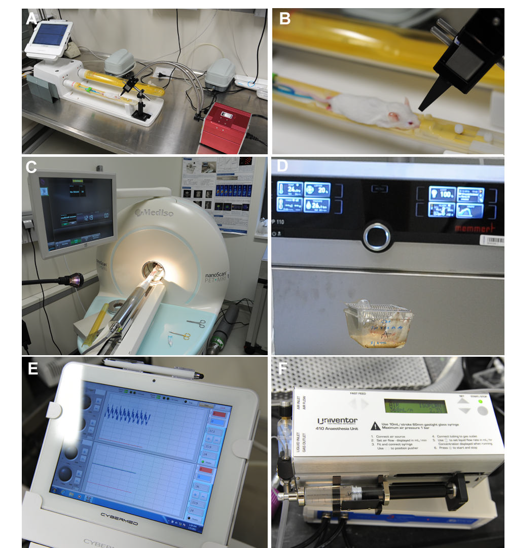
2.2. Light Stimulation Studies

The experimental setup for the fPET/MRI study was displayed in Figure 1 (A–F). The mice were placed in prone position on a special heated mouse pad with head affixed to a mouth piece (Figure 1A). The eyes were positioned and fixed for 20 min light stimulation through the double barrel of the light source Chromatoscope (Figure 1B) [1]. Subsequently, a whole body PET scan was started for a duration of 20 min using a preclincal scanner (Figure 1C). The animals were housed in an animal cabinet controlled day-light regimen with free access to food and water (Figure 1D). The respiration and anesthetic gas flow were monitored (Figure 1E,F).
The stimulation device is a custom-made double barrel tunnel placed around both eyes and the nose ridge to separate both visual fields, and has been described in detail elsewhere [1]. Both eyes were open at all times. At the end is a white screen illuminated by a remote light source. There is a groove before the screen that allows insertion of filters into the right and left visual fields respectively. The stimulation procedure has been described previously [1].

2.3. Color Vision Testing in Mice Using PET/MRI

The mouse retina contains two types of cones. Their pigments have spectral absorptions λmax of 360 nm (UV) and 510 nm, respectively [33]. The Wratten gelatine filter (#47), which has been used in the current study, has a passband for deep blue and UV. One may expect that primarily the deep blue signal reaches the retina, because the UV signal may not pass beyond the anterior of the eye. For color stimulation, the following Wratten filters (Kodak Photographic Filters) were used: deep blue (#47B, 452.7 nm) and deep yellow (#12, 510.7 nm). The mice were handled as described previously [1]. During stimulation the anesthetized animal had both eyes open and fixed while peering through the double barrel optic which has been coupled to a light source behind the white screen. To accomplish monocular deprivation for the short stimulation (20 min) one eye was covered with 5% dexpanthenol (Bepanthen, Bayer, Germany) to excite the contralateral eye only. Immediately before the stimulation, the animals obtained an injection of 12 ± 1 MBq [18F]FDG i.p. (courtesy Prof. M. Patt, Dept. Nuclear Medicine, University Hospital Leipzig, Leipzig, Germany). After finishing the stimulation, the PET scan -was performed for 20 min using the nanoScan®PET-MRI (Mediso Medical Imaging Systems, Budapest, Hungary) as described elsewhere [1].
Seven different stimulation conditions were performed:
  • dark: both eyes (1) closed (dark)
  • light: left (2) or right (3) eye open and subjected to standard light source (short: LightL, LightR)
  • blue: left (4) or right (5) eye open and subjected to standard light source with blue filter (short: BlueL, BlueR)
  • yellow: left (6) or right (7) eye open and subjected to standard light source with yellow filter (short: YellowL, YellowR).

2.4. Acquisition and Analysis of PET and MRI Data

Each PET image was corrected for random coincidences, dead time, scatter and attenuation. List-mode data were acquired and reconstructed as described previously [1]. Volume of interest (VOI) of various brain regions (right and left hemispheres, whole cortex, visual cortex) were defined on MRI-derived images by two observers using the software ROVER (ABX advanced biochemical compounds, Radeberg, Germany, v.2.1.15) [1,6]. First, a cylindrical VOI containing the whole cortex (Ctx) was drawn and center placed at the midline in coronal view of the PET/MR image (Figure 2A,B). This extends from the ventromedial occipital region through the posterior inferior temporal cortex. Two smaller VOIs were drawn from the center to the right border (visCtxR) and to the left border (visCtxL) of the Ctx region. Regional [18F]FDG uptake was calculated as standardized uptake value (SUV) [33] which comprises the ratio of the tissue activity concentration (kBq/g) and the injected radiotracer amount divided by the body weight. It was investigated at four mid-frame time points: 29.5, 34.5, 39.5 and 44.5 min, after the [18F]FDG administration. SUV was calculated for males (group A) and females (group B) for all color stimulation conditions mentioned above and for right (visCtxR) and left visual cortex (visCtxL).

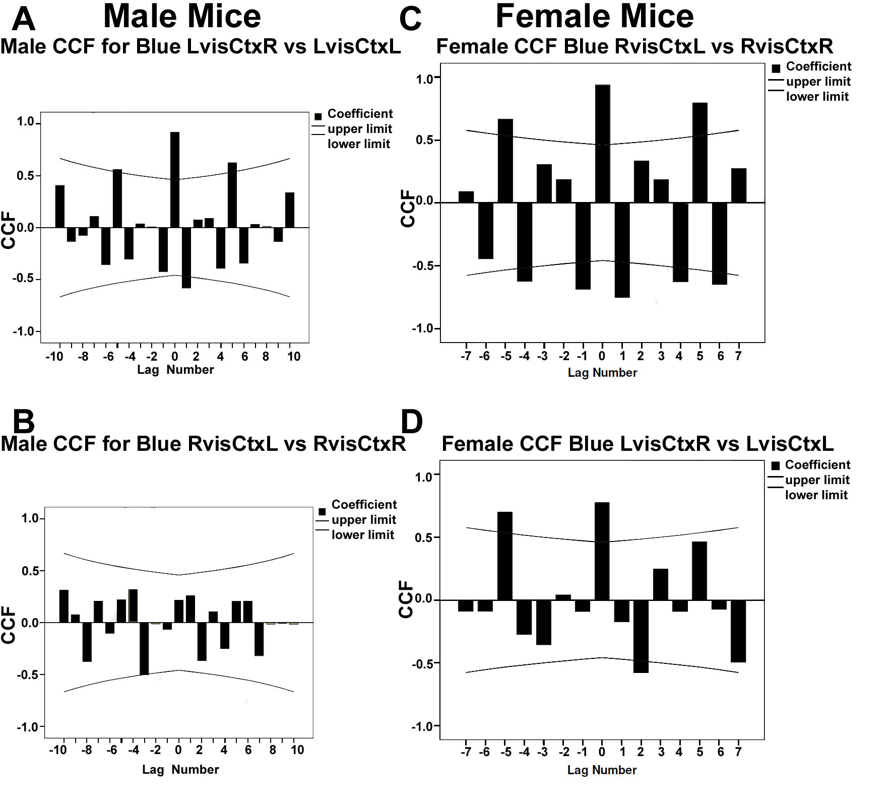
2.5. Statistical Analysis

Results were given as mean ± SD and plots represented as Mean/SE/1.96*SE where applicable. Stimulus effects were assessed by paired t-test statistics of stimulus condition compared to dark condition, and one-way analysis of variance (ANOVA); the alpha level was at 0.05. Multivariate Analysis of Variance (MANOVA) with repeated measures was applied. The latter was followed by planned t-tests to examine specific differences. The alpha level was at 0.05.

Stationarity Assumption

To examine the stationarity assumption of the time series, we applied the Augmented Dickey-Fuller (ADF) test using the software package STATA (Stata Corp LLC, College Station, TX, USA). Unit roots can cause unpredictable results in the data of a time series analysis. The ADF test is the unit root test for stationarity [31]. The ADF is applied because it can handle more complex models that the Dickey-Fuller test, and it is more powerful. However, it has a relatively high Type I error rate (i.e incorrect rejection true null hypothesis). After inspection of the dataset we chose the appropriate regression model, with constant. The ADF adds lagged differences to these models. In general, the ADF test is similar to the Dickey-Fuller test, using the model:
Δyt = α + βt + γyt − 1 + δ1Δy t − 1+ … + δp − 1Δyt − p + 1 + εt
where α is a constant, β the coefficient on a time trend and p the lag order of the autoregressive process. Imposing the constraints α = 0 and β = 0 corresponds to modeling a random walk and using the constraint β = 0 corresponds to modeling a random walk with a drift. We chose a lag length so that the residuals were not correlated. By including the lags of the order p the ADF formulation allows for higher-order autoregressive processes. This means that the lag length p has to be determined when applying the test. We used the t-statistic associated with the Ordinary least squares estimate of γ. The level of significance was set at 0.05. The null hypothesis of the Augmented Dickey-Fuller t-test is:
  • H0:γ = 0 (i.e., the data needs to be differenced to make it stationary);
  • H1: γ < 0 (i.e., the data is stationary and does not need to be differenced).
The Dickey-Fuller t-test statistic (DFT) was compared with the tabulated critical value [31]. If the DFT statistic is more negative than the table value, reject the null hypothesis of a unit root. The DFT statistic suggest that the time series data were strongly stationary without transformation.
D F T = γ ^ S E ( γ ^ )  

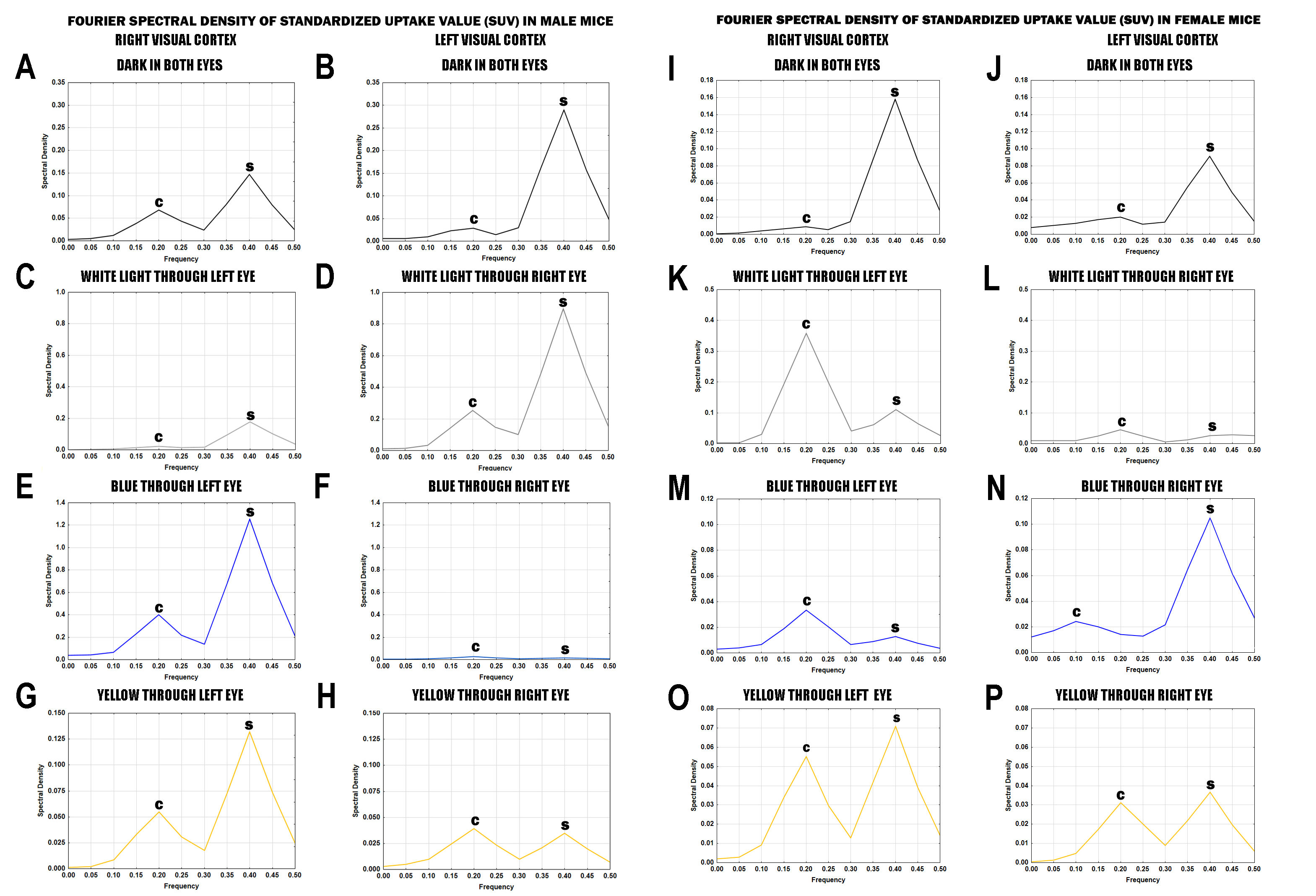
2.6. Fourier Analysis

The spectrum analysis was applied to examine the cyclical patterns of data of the mean ± SD SUV values. The rationale for exploration of the cyclical components is that it may correlate to the frequency of neuronal discharges in a given region of the brain during the observed phenomenon. It is hoped that we could uncover just a few recurring cycles of different lengths in the time series of metabolic activity that may reveal the seemly random noise of neuronal activity. The Fourier transform algorithm was applied using standard software (Time series and forecasting module, Statistica for Windows, StatSoft, OK, USA). All other analyses were performed using the software packages Statistica for Windows (StatSoft, OK, USA) and SPSS Version 20.0, (IBM SPSS Statistics for Windows, IBM Corp., Armonk, NY, USA). The spectrum analysis was applied to the SUV values provided in Table 1, to obtain spectral density coefficients given in Table 2, in male and female mice respectively. Fourier Spectral Density obtained during Dark condition and stimulation with white light, blue and yellow color in male and female mice, respectively.
The purpose of the Fourier analysis is to decompose the original time series into underlying sine and cosine functions of different frequencies, so as to identify the important frequency region. The wavelength of a sine or cosine function expressed as the number of cycles per unit time (frequency) is denoted as v. The period T of a sine or cosine function is defined by the length of time required for one full cycle. Thus, the period T is the reciprocal of frequency, or T = 1/v. One approach used is to restate the matter as a linear multiple regression model where the dependent variable is the observed time series, and the independent variables are the sine functions of all possible (discrete) frequencies. Thus the multiple regression model could be expressed as:
  x t = a 0 + k = 1 q   [ a k   ×   cos ( λ   ×   t ) + b k   ×   sin ( λ   ×   t ) ]  
The notation lambda (λ) is the frequency expressed in radians per unit time, given by = 2 × π × ν, where π = 3.1416. The cosine parameters ak and sine parameters bk are regression coefficients that indicate the degree of correlation with the data. There are q different sine and cosine functions; of which there are n/2 + 1 cosine functions and n/2 − 1 sine functions. This would mean that there would be many different sinusoidal waves as there are data points that would be able to completely replicate the series from the underlying functions. If the number of data points in the series is odd, then the last data point is ignored; and there must be at least two data points of high peak and low trough for a sinusoidal function to be identified. In other words, the standard and most efficient Fourier algorithm requires that the length of the input series is equal to a power of 2 [24]. If this is not the case, additional computations have to be performed. Fourier analysis will identify the correlation of sine and cosine functions of different frequencies within the observed data. If a large correlation is identified it could be said that there is strong periodicity of the respective frequency in the data.
The Fourier series states that any periodic function (or signal) can be expressed as a summation of orthogonal pair of matrices with one fundamental frequency and infinite number of harmonics. In other words, the sine and cosine functions are mutually independent (or orthogonal), thus the squared coefficients of each frequency may be summed to obtain the periodogram:
Pk = ak2 × bk2 × n/2
where Pk is the periodogram value at frequency vk and n is the overall length of the series. However, the periodogram values are subject to substantial random fluctuation that could yield many chaotic periodogram spikes. Hence, in practice, the plots utilized are the frequencies with the greatest spectral densities; that is, the frequency regions consisting of many adjacent frequencies that contribute most to the overall periodic behavior of the series. This is accomplished by smoothing the periodogram values via a weighted moving average transformation. The Hamming window is most often applied for this purpose.
The Hamming window is a modified Hanning window that belongs to the family of windows dependent upon the parameter α, with α normally being an integer [32]. As α becomes larger, the windows become smoother and the transform reflects this smoothness in decreased sidelobe level and faster falloff of the side lobes, but with an increased width of the main lobe. A perfect cancellation of the first side lobe (at θ = 2.5[2π/N]) occurs when α = 25/46 (α = 0.54). The N is the number of samples. When α is selected as 0.54, the new zero occurs at θ = 2.5[2π/N] and a marked improvement in side lobe level is achieved and for this value of α, the window is called Hamming window. In the Hamming window for each frequency, the weights for the weighted moving average of the periodogram values are computed as follows:
w(n) = 0.54 + 0.46 × cos × 2π/N × n n = −N/2, …, −1, 0, 1, …, N/2
w(n) = 0.54 − 0.46 × cos × 2π/N × n n = 0, 1, …, N − 1
The coefficients of the Hamming windows are nearly the set which achieve minimum side lobe levels. The approximation of the coefficients to two decimal places substantially lowers the level of side lobes to nearly equiripple condition. In the equiripple sense, the weights were optimally chosen as α = 0.53836 and α = 0.46164 [32,33]. All weight functions will assign the greatest weight to the observation being smoothed in the center of the window and increasingly smaller weights to values that are further away from the center. A ‘white noise’ input series will result in periodogram values that follow an exponential distribution.
Cross spectrum analysis was implemented to determine the relationship between the two times series in the left and right visual cortex during blue light stimulation to the right and left eye, in male and female mice, respectively. The cross correlation function (CCF) was calculated as the correlation of the time series for the pairs: left visual cortex through the right eye (RvisCtxL) with right visual cortex through the right eye (RvisCtxR); and left eye in the right visual cortex (LvisCtxR) with left eye in the left visual cortex (LvisCtxL), shifted by a particular number of observations, in male and female mice, respectively. The cross amplitude values were computed as the square root of the sum of the squared cross-density and quad-density values. It was interpreted as a measure of the covariance between the respective frequency components in the two series. The phase spectrum estimates show the extent to which each frequency component of one series leads the other. The gain was interpreted as the standard least squares regression coefficient for the respective frequencies. The squared coherency was interpreted as the squared correlation coefficient of the two time series in the given context.

2.7. Software Procedure for Data Analysis

To obtain the required time series, the 20 data points for each stimulus condition were analyzed for males and females, respectively. The analysis begins in Fourier Analysis dialog window, by choosing spectral density estimates and the Hamming window, then Plot to display cyclical patterns in male and female mice, respectively. The spectral density estimates, derived from single series Fourier analysis were plotted, and the frequency regions with the highest estimates were marked as peaks. The spectral density estimates between two minima including the peak (as maxima) were analyzed to examine the effects of stimuli on cortical and subcortical sites. The spectral density peaks were identified as cortical (C-peak) and subcortical (S-peaks) whose peaks occurred at regular frequency intervals of 0.2 and 0.4, respectively. For evaluation of stimulus responses, the area under the curve derived for a particular stimulus was compared to that derived from another stimulus. Further statistical analysis was carried out using the five data points from trough-to-peak-to-trough for the C-peak and S-peak, respectively, as shown in Table 2.

3. Results

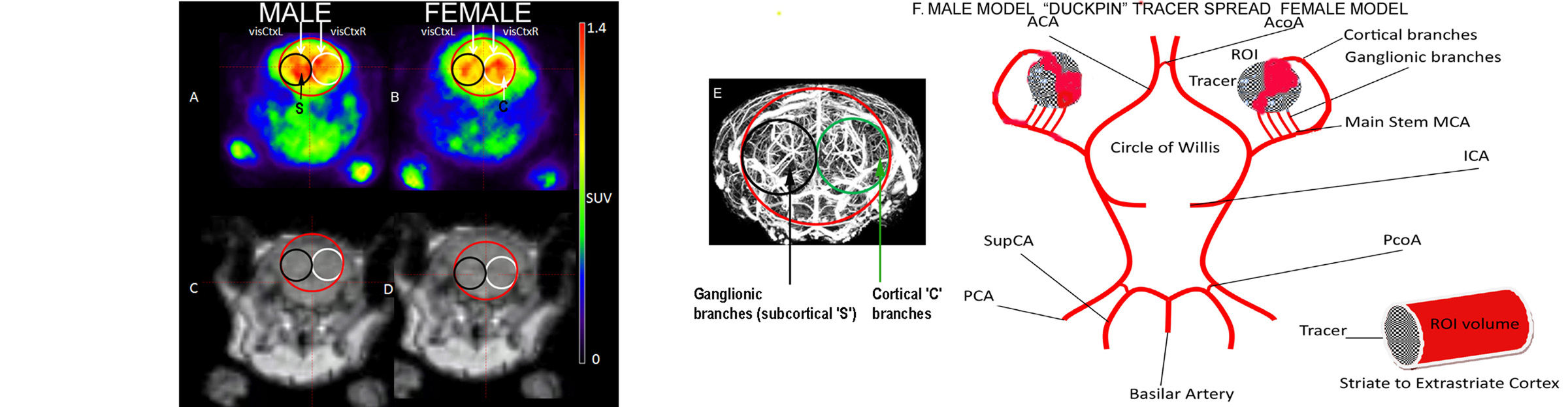
3.1. Analysis of fPET/MRI Images

Figure 2A,B show the fPET/MRI images (Figure 2A) and volumes of interest (VOI) in mouse cerebral vasculature by X-ray micro-computerized tomography (micro-CT) (Figure 2B). In male mice, Figure 2A (black circle) shows a tracer distribution in the left visual cortex (visCtxL) that is shaped like a Canadian ‘duckpin’ with a short small head at the top dorsal cortical region, a narrow neck (open arrow), and a long fat base into a wide area of spread in the central ventral subcortical region during Blue light stimulation. In male mice, the “upright Canadian duckpin” tracer spread may suggest a small focal brain area of ‘arousal’ at the head placed within the dorsal cortical region of the left visual cortex and at the base a secondary wide area of spread in the subcortical region. On the other side, in the right visual cortex (visCtxR) there is intense concentration of tracer and no peculiar organization of the tracer distribution. In female mice, Figure 2B (white circle) shows an “inverted Canadian duckpin” tracer distribution in the right visual cortex (visCtxR) with a small area of “arousal” at the head placed within the subcortical region in the right visual cortex and at the base in the dorsal tempero-occipital cortical region. The contralateral left visual cortex (visCtxL) does not show any remarkable tracer distribution.
Figure 2C,D shows the MRI images in male (Figure 2C) and female (Figure 2D) mice used for anatomic orientation. Figure 2E, shows the VOI setup in mouse brain on micro-CT image [34] in coronal view. The figure illustrates the VOIs used for data analysis in relation to the brain vessel system, red: Ctx, black: visCtxL and green: visCtxR. Visual observation due to low image resolution could not clearly delineate vascular territories and borders of cortical and subcortical distribution. Hence, more reliable methods are needed. Figure 2F, shows the schematic diagram of the arterial tree of the Circle of Willis and the relationship to the region of interest (ROI) to the cortical and ganglionic branches of the middle cerebral artery in the mouse brain. The left side of the Circle of Willis shows the ‘male model’ of radiotracer distribution, while the right side shows the ‘female model’.

3.2. Analysis of Mean SUV Data

We analyzed the mean ± SD SUV data obtained in direct measurements in male (Table 1 top panel) and female mice (Table 1 bottom panel), respectively. A MANOVA with repeated measures was performed on the mean ± SD SUV values, with a 7 × 2 × 2 design: seven levels of stimulation of the visual cortex, Stimulations (Dark, Light R, Light L, Blue R, Blue L, Yellow R, Yellow L), two levels of Visual Cortex (visCtxR, visCtxL) and two levels of Gender (male and female), with the mean ± SD SUV during stimulations were analyzed as the dependent variable. There were main effects of Stimulations, F(6,228) = 7.621, MS = 0.356, p < 0.0000001; Visual Cortex, F(1,38) = 7.157; MS = 0.026; p < 0.05; and Gender, (F(1,38) = 15.15, MS = 2.065, p < 0.001. There was a Stimulation x Gender interaction, F(6,228) = 6.405, MS = 0.299, p < 0.0001). There was also a Stimulations x Visual Cortex interaction F(6,228) = 4.21, MS = 0.0141, p < 0.001. The analysis of mean ± SD values of SUV detected changes related to the overall effects of visual stimulations in the visual cortex but did not distinguish changes in the dorsal and ventral streams, respectively.

3.3. Analysis of Spectral Density Data

The spectral density data obtained from the time series analysis SUV values (Table 1) are provided for male and female (Table 2). A MANOVA with repeated measures was performed with a 7 × 2 × 2 × 2 design: seven levels of Stimulations (Dark, Light R, Light L, Blue R, Blue L, Yellow R, Yellow L), two levels of Visual Cortex (visCtxR, visCtxL), two levels of Peaks (C-peak, S-peak) and two levels of Gender (male, female). There was a main effect of Stimulations, F(6,102) = 8.65, MS = 0.094, p < 0.0000001. There was a Stimulations x Gender interaction, F(6,102) = 7.68, MS = 0.083, p < 0.000001. There was a Stimulations x Visual Cortex x Gender interaction, F(6,102) = 3.4, MS = 0.00098, p < 0.01. There was a Stimulations x Visual Cortex x Peaks interaction, F(6,102) = 3.4, MS = 0.00075, p < 0.01. Fourier spectral density analysis demonstrated the overall effects. Further analysis was undertaken to show specific effects of spatial opponency, luminance opponency and chromatic opponency during visual stimulations in the visual cortex in the dorsal (cortical C-peak) and ventral (subcortical S-peak) streams, respectively. Detection of these effects would dramatically improve the temporal and spatial resolutions of conventional PET/MRI imaging.

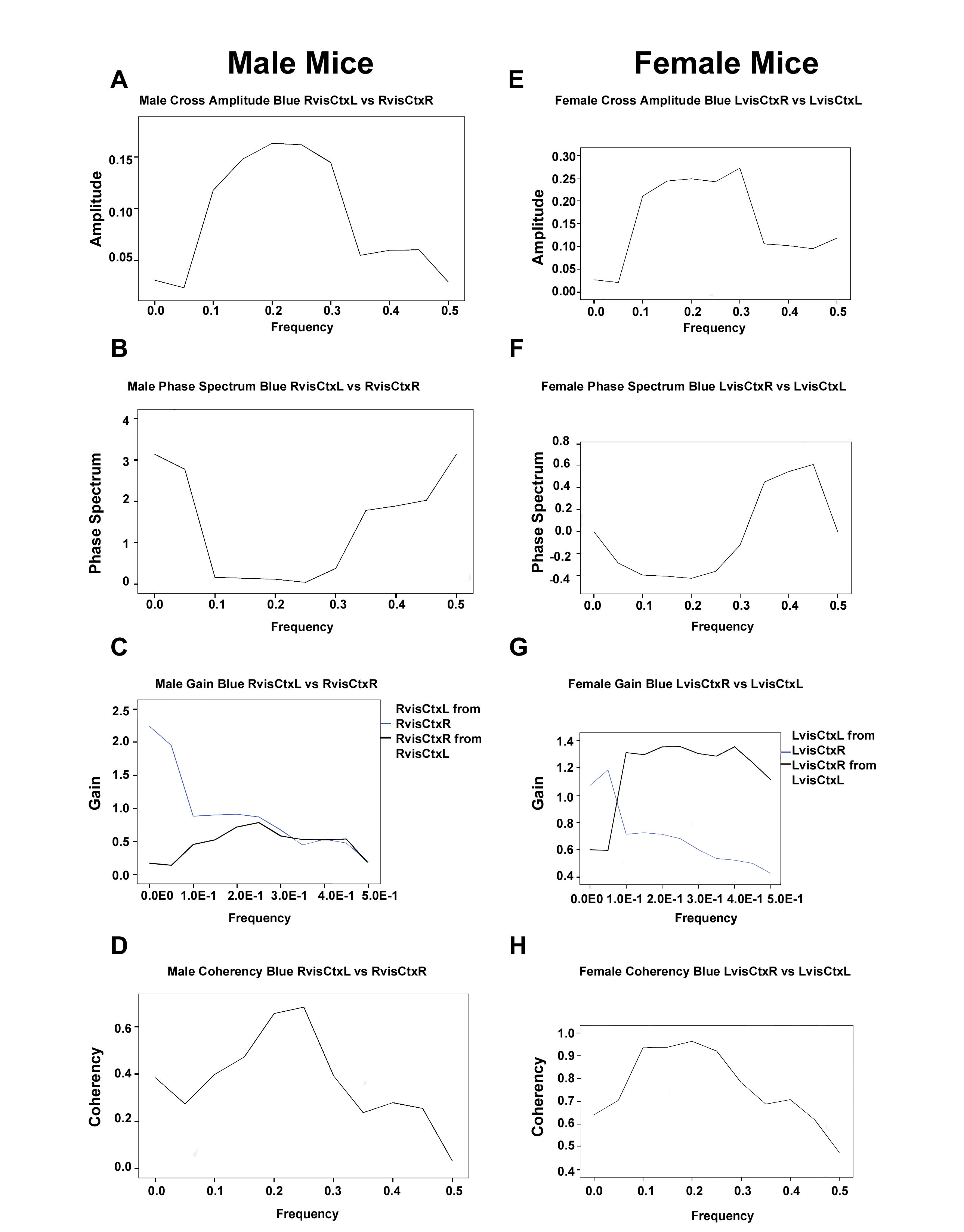
3.3.1. Analysis of Spectral Density Data in Male Mice

In male mice, Table 3 (top panel) demonstrates spatial, luminance and chromatic opponency determined by Fourier spectral density coefficients (mean ± SD) values in paired t-test results in the right visual cortex through the left eye (LvisCtxR) and left visual cortex through the right eye (RvisCtxL), and percentage changes from the Dark condition (Δ%Dark). Figure 3A–H shows the spectral density plots of Fourier coefficients. In male mice, under the Dark condition, while there was no significant difference in amplitudes between C-peak and S-peak in the right visual cortex (visCtxR) (Figure 3A), in the left visual cortex (visCtxL) (Figure 3B), the S-peak was significantly higher than the C-peak, which demonstrated spatial opponency, (p < 0.05).
During White light stimulation through the left eye in the right visual cortex (LvisCtxR) (Figure 3C), the C-peak was attenuated by −66.7%, (p < 0.05), with no significant change in S-peak, but resulted in significant presence of spatial opponency, (p < 0.05). During stimulation with White light through the right eye in the left visual cortex (RvisCtxL) (Figure 3D), there was accentuation of S-peak by 210%, (p < 0.05), which in comparison to Dark condition induced luminance opponency, (p < 0.05), in the subcortical region in the ventral stream. Luminance opponency was present in the cortico-subcortical circuit of combined contrast using C-peak and S-peak, (p < 0.05). During stimulation with Blue light through the left eye in the right visual cortex (LvisCtxR) (Figure 3E), there was attenuation of C-peak by −21%, (p < 0.05), but no significant change in S-peak. However, during stimulation with Blue light through the right eye in the left visual cortex (RvisCtxL) (Figure 3F), there was no significant change in C-peak, but the S-peak was remarkable attenuated by −92.7%, (p < 0.05). During stimulation with Yellow light through the left eye in the right visual cortex (LvisCtxR) (Figure 3G), the C-peak was attenuated by −21%, (p < 0.05), and S-peak was also attenuated by −9.8%, (p < 0.05). However, during stimulation with Yellow light through the right eye in the left visual cortex (RvisCtxL) (Figure 3H), the C-peak did not change significantly, but there was a marked attenuation of the S-peak by −87%, (p < 0.05). In other words, during stimulation with the Blue/Yellow pairs, there was marked attenuation of C-peaks and S-peaks across brain regions but not the C-peaks in the left visual cortex through the right eye (RvisCtxL), which resulted in significant differences between Blue versus Yellow for chromatic opponency, (p < 0.05) in the cortical region in the dorsal stream. The chromatic opponency was present in the cortico-subcortical circuit of combined C-peak and S-peak Blue/Yellow contrast, (p < 0.01). Spatial opponency was not elicited during stimulation with Blue and Yellow colors.
Overall, in male mice, luminance opponency was implemented in the subcortical region of the left visual cortex in the ventral stream, while chromatic opponency was present in the cortical region of the left visual cortex in the dorsal stream.
Cross spectrum analysis with Blue light stimulation demonstrated consistent findings in both male and female. Cross spectrum analysis in male mice is displayed in Figure 4A,B and Figure 5A–D. Figure 4A shows the CCF for Blue light stimulation for the pair LvisCtxR vs. LvisCtxL. In Figure 4A for the pair LvisCtxR vs. LvisctxL, CCF shows strong positive correlation at −5, 0, +5 lags, and strong negative correlation at +1 lag. This activation pattern was associated with regions not specifically implicated in Blue light stimulation in male mice. On the other hand, regions implicated in Blue light stimulation as demonstrated in Figure 4B for the pair RvisctxL vs. RvisCtxR, showed that the CCF was negatively correlated at −3 lag.
Further analysis of the effects of Blue light stimulation was demonstrated in Figure 5(A–D), and shows the cross amplitude (Figure 5A), phase spectrum (Figure 5B), gain (Figure 5C) and coherency (Figure 5D) for the RvisCtxL vs. RvisCtxR pairs. Figure 5A, shows that the cross amplitude was highest in the lower frequency range from 0.1 to 0.3, and diminished by about one-third in the higher frequency from 0.35 to 0.5. Figure 5B, demonstrates that the phase spectrum was least in the lower frequency range from 0.1 to 0.3, and increased in the higher frequency range of 0.35 to 0.5. Figure 5C, shows that the gain reduced across the lower and higher frequency range from 1.0 × 10⁻¹ to 5.0 × 10⁻¹, which may suggest that both time series constitute predominantly of similar component waveforms with no amplification. Figure 5D shows that the coherency was very high in the very narrow frequency range from 0.2 to 0.25, exceeding by three times the coherency in the higher frequency range from 0.35 to 0.5. In other words, in male mice, the cross spectrum analysis suggests that Blue light stimulation caused specific changes of ‘spectral narrowing’ in the lower frequency range.

3.3.2. Analysis of Spectral Density Data in Female Mice
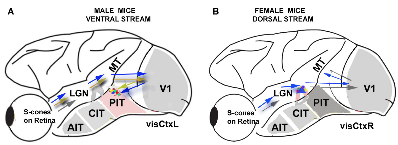
In female mice, Table 3 (bottom panel) demonstrates spatial, luminance and chromatic opponency determined by Fourier spectral density coefficients (mean ± SD) values in paired t-test results in the right visual cortex through the left eye (LvisCtxR) and left visual cortex through the right eye (RvisCtxL), and percent changes from Dark condition (Δ% Dark). In female mice, under Dark condition, there was significant difference in amplitudes in the right visual cortex (visCtxR) (Figure 3I), the S-peak was significantly higher than the C-peak, which demonstrated spatial opponency, (p < 0.05). On the other hand, in the left visual cortex (visCtxL) (Figure 3J), the C-peak and S-peak were not significantly different. During White light stimulation in the right visual cortex through the left eye (LvisCtxR) (Figure 3K), there was marked broad-spectrum accentuation of C-peak by 3020% with a wide range of standard deviation (SD) and was not significantly different from Dark condition. There was a wide range of spectral densities below the area of the curve (Figure 3K), which in turn indicates a broad spectrum of constituent frequencies activated by the broad spectra of White light photonic frequencies from low to very high with no selective response. In the contralateral left visual cortex through the right eye (RvisCtxL), both C-peak and S-peak were not significantly different from Dark condition. During stimulation with Blue light through the left eye in the right visual cortex (LvisCtxR) in female mice (Figure 3M), there was significant accentuation of C-peak by 220%, (p < 0.05), and attenuation of S-peak by −90.5%, (p < 0.05), suggestive of a selective response to the high-frequency Blue light. In the contralateral left visual cortex through the right eye (RvisCtxL) (Figure 3N), the changes were not significantly higher than for the Dark condition, but with a tendency for attenuation of C-peak and accentuation of S-peak which created a condition for spatial opponency, (p < 0.05). During stimulation with Yellow light through the left eye in the right visual cortex (LvisCtxR) (Figure 3O), the C-peak and S-peak were not significantly different from that in the Dark condition. During stimulation with Yellow light through the right eye in the left visual cortex (RvisCtxL) (Figure 3P), there was no significant change in C-peak, but a significant attenuation of S-peak by −75%, (p < 0.05). The chromatic opponency of Blue/Yellow pairs was present in the subcortical region (S-peak) in the ventral stream in the right visual cortex, (p < 0.05). The chromatic opponency was implemented in the cortico-subcortical circuit of combined C-peak and S-peak Blue/Yellow contrast, (p < 0.01). Overall, in female mice, the response to Blue light stimulation was frequency-modulated which induced resonance phenomenon [35] in the cortical region in the dorsal stream of the right visual cortex, while in the subcortical region in the ventral stream in the right visual cortex, chromatic opponency was implemented.
Cross spectrum analysis in female mice is displayed in Figure 4C,D and Figure 5E–H. Figure 4C shows the CCF for Blue light stimulation for the pair RvisCtxL vs. RvisCtxR. In Figure 4C for the pair RvisCtxL vs. RvisCtxR, CCF shows strong positive correlation at −5, 0, +5 lags, and strong negative correlation at −4, −1, +1, +4, +6 lags. This activation pattern was associated with regions not directly implicated in Blue light stimulation in female mice. On the other hand, regions directly implicated in Blue light stimulation as demonstrated in Figure 4D for the pair LvisCtxR vs. LvisCtxL, showed that the CCF was strongly positively correlated at −5 and 0 lags, and strongly negatively correlated at +2 lag, distinct from that seen in male mice.
Further analysis of the effects of Blue light stimulation was demonstrated in Figure 5(E–H), and shows the cross amplitude (Figure 5E), phase spectrum (Figure 5F), gain (Figure 5G) and coherency (Figure 5H) for the pairs LvisCtxR vs. LvisCtxL. Figure 5E, shows that the cross amplitude was highest in the lower frequency range from 0.1 to 0.3, and diminished by twice in the higher frequency range from 0.35 to 0.45, compared to the relatively much lower levels in male mice. Figure 5F, demonstrates that the phase spectrum was least in the lower frequency range of 0.1 to 0.2 and highest in the higher frequency range of 0.35 to 0.5. Figure 5G, shows that the gain for the pair LvisCtxR from LvisCtxL was significantly amplified compared to the pair LvisCtxL from LvisCtxR, across the lower and higher frequencies from 1.0 × 10⁻¹ to 5.0 × 10⁻¹. This may suggest that both time series constitute different component waveforms with amplification of LvisCtxR. Figure 5H, shows the coherency was highest with ‘spectral broadening’ in the lower frequency range from 0.1 to 0.3. In the higher frequency range from 0.35 to 0.5, the coherency increased to the two-third level of that in the lower frequency range. In other words, in contrast to the male pattern, in female mice, coherency increased with ‘spectral broadening’ across the lower and higher frequency range.

4. Discussion

4.1. Gender Differences in Mechanisms for Color Processing

There were novel gender differences in white light and color processing. The frequency-related resonance phenomenon [35] while present in female mice was absent in male mice, that is, female mice had preference for processing the frequency of particles of light, while male mice has the preference of processing the wavelength of light. In other words, male mice differentiated color light stimulus by wavelength-differencing, while female mice implemented frequency-differencing [18,19]. The gender differential processing of light as a wave and as a particle to our knowledge has not be firmly established [17,18,19], and requires further studies, because of the potential implications for understanding the differences in processing in the visual sensory system. We postulate that, there are two separate male (Figure 6A) and female (Figure 6B) models for white light and color processing in the mouse brain, shown in the schematic diagram (Figure 6 A,B).
Figure 6A shows the male mouse model, comprising a wavelength-differencing system that receive inputs from retinal S-cones on activation of the visual pathway from the retina, through the dorsal lateral geniculate nucleus of the thalamus (LGN) to the primary visual cortex (V1) traversing the associative visual areas (V2, V3) and areas like the fusiform gyrus and lingual gyrus with others collectively referred to as visual area 4 (V4), to the angular gyrus implicated in the higher order processing of colors along the ventral stream [36] through posterior (PIT), central (CIT) and anterior inferior temporal (AIT) cortex in the left hemisphere of the brain. The color processing is accomplished between two color spaces by wavelength-sensitive cortical neurons with axons in the cortical-subcortical circuits. The inferior temporal (IT) contains regions that are relatively more responsive to color (seen in Figure 6A as an area checkered with colors in PIT). The ventral pathway is thought to represent stable attributes of objects (object quality) [36,37]. The processing of luminance takes place within the retino-subcortical circuits by light-sensitive subcortical neurons. Female mice demonstrate a frequency-differencing system by neurons in the subcortical region that differentiate high frequency color, such as blue from low frequency color such as yellow. Figure 6B, shows the schematic model in female mice, which demonstrates retino-subcortico-cortical circuits that receive inputs from the retinal S-cones on activation of the visual pathway from the retina to specialized frequency-selective neurons in the dorsal lateral geniculate nucleus of the thalamus (LGN), with axons ascending within the dorsal stream to the primary visual cortex (V1) and middle temporal (MT) area in the right hemisphere of the brain, involved primarily in the detection of motion. Conventionally, it is presumed that, the dorsal stream was implicated in encoding dynamic spatiotemporal relationships among visual objects (object action) [36,37].

4.2. Fourier Analysis to Differentiate Cortical and Ganglionic Vessels

The primary questions were to resolve the origins of C-peak and S-peak, their anatomic correlates and functional significance. The C-peak and S-peak occurred at multiples of the first harmonic or the fundamental frequency, at the second and third harmonics, respectively. It has been demonstrated that, in the vascular system, the first five harmonics contain 90% percent of the pulsatile energy of the system [38]. These frequencies could be converted to cycles per second (Hz), assuming that the fundamental frequency of cardiac oscillation was the mean heart rate. The fundamental frequency f of the first harmonic was determined by the mean heart rate per second of CD-1 mice = 515 ± 30 bpm/60 s = 8.6 Hz [38]. Thus, the distance of the reflection site for fundamental frequency could be presumed to emanate from a site at D1 = =1/4 λ or c/4f, or 1.91m/s/(4 × 8.6 Hz) = 0.055 m/s or 5.5 cm; where c = 1.91 ± 0.44 m/s, is the wave propagation velocity [39]. These distances are not physical measurements but approximate the actual arterial lengths. Taking into account vascular tortuosity, the estimated distance (5.5 cm) approximates that from the terminal vessels in the brain, to an imaginary site of summed reflections from the aorto-iliac junction of the mice. The C-peak occurred at the second harmonic, such that, the estimated arterial length given by D2 = 1/8 λ or c/8 × 2f, or 1.91 m/s/(8 × (2 × 8.6 Hz or 17.2 Hz)) = 0.0139 m or 1.4 cm, approximates the visible arterial length from the main stem of the major cortical arteries around the cerebral convexity to the end occipito-temporal junction as shown in mouse brain [34]. The cortical frequency of 17 Hz is within the beta rhythm range (~14–18 Hz) said to be implicated in cortical areas of higher visual hierarchy in top-down feed-back processing [40] in the visual system. Thus it is implied that beta rhythms could predominate in cortico-subcortical patterns of activation in male mice. The S-peak occurred at the third harmonic, such that the estimated arterial length given by D3/= 1/16 λ or c/16 × 3f, or 1.91 m/s /(16 × (3 × 8.6 Hz or 25.8 Hz)) = 0.0046 m or 0.46 cm or 4.6 mm, which approximates the visible arterial length from the main stem of the major cortical arteries to the distal arterioles of the ganglionic branches [34]. The 25 Hz is the frequency of the rhythm of gamma waves [40]. The ratio of the length of the ganglionic branches to the cortical branches is 1:3 in mice. The same ratio has been found in human subjects [20]. This may suggest that the cerebral vaso-architecture was optimized in mammals to facilitate harmonic oscillations within the cortico-subcortical networks.

5. Conclusions

The findings suggest that during color stimulation there was enhancement of the cortical C-peak in the lower frequency range which correlates with 17 Hz beta-band synchronization in the left visual cortex in male mice. Conversely, in female mice, there was ‘spectral broadening’ and accentuation of subcortical S-peak in the higher frequency range which correlates with 25 Hz gamma-band synchronization [40] in the right visual cortex. These present findings agree with recordings of neuronal cortical beta-band and subcortical gamma-band synchronization in neuronal computation [40], consistent with the input function from gamma aminobutyric acid (GABA) modulation of color-opponent bipolar cells in the retina [41,42]. Furthermore, the present work demonstrated that Fourier time-series analysis is a computational approach that could be implemented in the visual system for light and color processing. Fourier analysis of mean SUV of [18F]FDG [43] have improved the use of fPET/MRI to index the coupling of rCBF, CMRO2 and neuronal activity with a wide range of applications in several areas of cognitive neuroscience [44].
Of particular interest is the hypothesis suggesting that the main gender differential in color memory mechanisms is input into memory formation processes in male mice, but output retrieval of memory in female mice. This may suggest that color processing could be of immense use in diagnosis of brain degenerative diseases and depression, and further extend the possibilities of development and testing of new memory drug targets within the hippocampus [45]. The findings could also apply to methodologies of artificial intelligence and human–computer interface, as well as understanding the relationships of quantum mechanics and human perception of conscious experience. The very important principle of cerebal asymmetry implying gender complimentarity was demonstrated in humans for color [18,19], facial [20] and general intelliegence [46] processing, and now has been upheld in the present study for color processing in the mice model [1]. To explain these findings, a light hypothesis for cerebral asymmetry was postulated, which posits that, the phenotypic neuroadaptation to the environmental physical constraints of light wave/particle duality, led to phenotypic evolution and genetic variation of X-Y gene pairs that determined cerebral asymmetry for brain functions in both males and females. The evolutionary trend is towards optimization of perception of the ‘whole’ environment by functional coupling of the genes for complementarity of both hemispheres within self, and between genders [18,19].

Author Contributions

Conceptualization, P.C.N. and P.B.; Methodology, P.C.N., and M.K.; Software, P.C.N. and M.K.; Validation, P.C.N., M.K. and P.B.; Formal Analysis, P.C.N.; Investigation, P.C.N. and M.K.; Resources, P.C.N. and P.B.; Data Curation, P.B.; Writing-Original Draft Preparation, P.C.N.; Writing-Review & Editing, P.C.N. and P.B.; Visualization, P.C.N. and M.K.; Supervision, P.B.; Project Administration, P.C.N., and P.B.; Funding Acquisition, P.C.N. and P.B.

Funding

This research received no external funding.

Conflicts of Interest

The authors declare no conflict of interest.

References

  1. Njemanze, P.C.; Kranz, M.; Amend, M.; Hauser, J.; Wehrl, H.; Brust, P. Gender differences in cerebral metabolism for color processing in mice: A PET/MRI study. PLoS ONE 2017, 12, e0179919. [Google Scholar] [CrossRef] [PubMed]
  2. Ungerleider, L.G.; Haxby, J.V. ‘What’ and ‘where’ in the human brain. Curr. Opin. Neurobiol. 1994, 4, 157–165. [Google Scholar] [CrossRef]
  3. Ungerleider, L.G.; Mishkin, M. Two cortical visual systems. In Analysis of Visual Behavior; Goodale, M.A., Mansfield, R.J.Q., Eds.; MIT: Cambridge, MA, USA, 1982; pp. 549–586. [Google Scholar]
  4. Perry, C.J.; Fallah, M. Feature integration and object representations along the dorsal stream visual hierarchy. Front. Comput. Neurosci. 2014, 8, 84. [Google Scholar] [CrossRef] [PubMed]
  5. McKeefry, D.J.; Zeki, S. The position and topography of the human color centre as revealed by functional magnetic resonance imaging. Brain 1997, 120, 2229–2242. [Google Scholar] [CrossRef] [PubMed]
  6. Gray, H.; Clemente, C.D. Gray’s Anatomy of the Human Body, 30th American ed.; Lippincott Williams & Wilkins: Philadelphia, PA, USA, 1984; ISBN-13 978-0812106442. [Google Scholar]
  7. Takechi, H.; Onoe, H.; Shizuno, H.; Yoshikawa, E.; Sadato, N.; Tsukada, H.Y.; Watanabe, Y. Mapping of cortical areas involved in color vision in non-human primates. Neurosci. Lett. 1997, 230, 17–20. [Google Scholar] [CrossRef]
  8. Buchsbaum, G.; Gottschalk, A. Trichromacy, opponent colors coding and optimum color information transmission in the retina. Proc. R. Soc. Lond. B Biol. Sci. 1983, 220, 89–113. [Google Scholar] [CrossRef] [PubMed]
  9. Gouras, P. The Perception of Color: Vision and Dysfunction; Macmillan: England, UK, 1991; pp. 179–197. [Google Scholar]
  10. Daw, N.W. Goldfish retina: Organization for simultaneous color contrast. Science 1967, 158, 942–944. [Google Scholar] [CrossRef] [PubMed]
  11. Livingstone, M.S.; Hubel, D.H. Anatomy and physiology of a color system in the primate visual cortex. J. Neurosci. 1984, 4, 309–356. [Google Scholar] [CrossRef] [PubMed]
  12. Dufort, P.A.; Lumsden, C.J. Color categorization and color constancy in a neural network model of V4. Biol. Cybern. 1991, 65, 293–303. [Google Scholar] [CrossRef] [PubMed]
  13. Kraft, J.M.; Brainard, D.H. Mechanisms of color constancy under nearly natural viewing. Proc. Natl. Acad. Sci. USA 1999, 96, 307–312. [Google Scholar] [CrossRef] [PubMed] [Green Version]
  14. Conway, B.R. Spatial structure of cone inputs to color cells in alert macaque primary visual cortex (V-1). J. Neurosci. 2001, 21, 2768–2783. [Google Scholar] [CrossRef] [PubMed]
  15. Zeki, S. A Vision of the Brain; Plate 16; Blackwell Scientific: Cambridge, MA, USA, 1993. [Google Scholar]
  16. Njemanze, P.C.; Gomez, C.R.; Horenstein, S. Cerebral lateralization and color perception: A transcranial Doppler study. Cortex 1992, 28, 69–75. [Google Scholar] [CrossRef]
  17. Njemanze, P.C. Asymmetric neuroplasticity of color processing during head down rest: A functional transcranial Doppler spectroscopy study. J. Gravit. Physiol. 2008, 15, 49–59. [Google Scholar]
  18. Njemanze, P.C. Gender-related asymmetric brain vasomotor response to color stimulation: A functional transcranial Doppler spectroscopy study. Exp. Transl. Stroke Med. 2010, 2, e21. [Google Scholar] [CrossRef] [PubMed]
  19. Njemanze, P.C. Gender-related differences in physiologic color space: A functional transcranial Doppler (fTCD) study. Exp. Transl. Stroke Med. 2011, 3, e1. [Google Scholar] [CrossRef] [PubMed]
  20. Njemanze, P.C. Cerebral lateralisation for facial processing: Gender-related cognitive styles determined using Fourier analysis of mean cerebral blood flow velocity in the middle cerebral arteries. Laterality 2007, 12, 31–49. [Google Scholar] [CrossRef] [PubMed]
  21. Yarowsky, P.J.; Ingvar, D.H. Symposium summary. Neuronal activity and energy metabolism. Fed. Proc. 1981, 40, 2353–2362. [Google Scholar] [PubMed]
  22. Fox, P.T.; Raichle, M.E. Focal physiological uncoupling of cerebral blood flow and oxidative metabolism during somatosensory stimulation in human subjects. Proc. Natl. Acad. Sci. USA 1986, 83, 1140–1144. [Google Scholar] [CrossRef] [PubMed]
  23. Dahl, A.; Lindegaard, K.-F.; Russell, D.; Nyberg-Hansen, R.; Rootwelt, K.; Sorteberg, W.; Nornes, H. A comparison of transcranial Doppler and cerebral blood flow studies to assess cerebral vasoreactivity. Stroke 1992, 23, 15–19. [Google Scholar] [CrossRef] [PubMed]
  24. Bloomfield, P. Fourier Analysis of Time Series: An Introduction; Wiley: New York, NY, USA, 1976. [Google Scholar]
  25. Attinger, E.O.; Anne, A.; McDonald, D.A. Use of Fourier series for analysis of biological systems. Biophys. J. 1966, 6, 291–304. [Google Scholar] [CrossRef]
  26. Njemanze, P.C.; Beck, O.J.; Gomez, C.R.; Horenstein, S. Fourier analysis of the cerebrovascular system. Stroke 1991, 22, 721–726. [Google Scholar] [CrossRef] [PubMed]
  27. Schuett, S.; Bonhoeffer, T.; Hübener, M. Mapping retinotopic structure in mouse visual cortex with optical imaging. J. Neurosci. 2002, 22, 6549–6559. [Google Scholar] [CrossRef] [PubMed]
  28. Bastos, A.M.; Vezoli, J.; Bosman, C.A.; Schoffelen, J.M.; Oostenveld, R.; Dowdall, J.R.; De Weerd, P.; Kennedy, H.; Fries, P. Visual areas exert feedforward and feedback influences through distinct frequency channels. Neuron 2015, 85, 390–401. [Google Scholar] [CrossRef] [PubMed]
  29. Bliss, T.V.; Lomo, T. Long-lasting potentiation of synaptic transmission in the dentate area of the anaesthetized rabbit following stimulation of the perforant path. J. Physiol. 1973, 232, 331–356. [Google Scholar] [CrossRef] [PubMed] [Green Version]
  30. Ito, M. Long-term depression. Annu. Rev. Neurosci. 1989, 12, 85–102. [Google Scholar] [CrossRef] [PubMed]
  31. Kwiatkowski, D.; Phillips, P.C.B.; Schmidt, P.; Shin, Y. Testing the null hypothesis of stationarity against the alternative of a unit root: How sure are we that economic time series have a unit root? J. Econom. 1992, 54, 159–178. [Google Scholar] [CrossRef]
  32. Harris, F.J. On the use of windows for harmonic analysis with the discrete Fourier transform. Proc. IEEE 1978, 66, 51–83. [Google Scholar] [CrossRef] [Green Version]
  33. Poularikas, A.D. The Handbook of Formulas and Tables for Signal Processing; CRC Press LLC: Boca Raton, FL, USA, 1999. [Google Scholar]
  34. Ghanavati, S.; Yu, L.X.; Lerch, J.P.; Sled, J.G. A perfusion procedure for imaging of the mouse cerebral vasculature by X-ray micro-CT. J. Neurosci. Methods 2014, 221, 70–77. [Google Scholar] [CrossRef] [PubMed] [Green Version]
  35. Hutcheon, B.; Yarom, Y. Resonance, oscillation and the intrinsic frequency preferences of neurons. Trends Neurosci. 2000, 23, 216–222. [Google Scholar] [CrossRef]
  36. DiCarlo, J.J.; Zoccolan, D.; Rust, N.C. How does the brain solve visual object recognition? Neuron 2012, 73, 415–434. [Google Scholar] [CrossRef] [PubMed]
  37. Kravitz, D.J.; Saleem, K.S.; Baker, C.I.; Mishkin, M. A new neural framework for visuospatial processing. Nat. Rev. Neurosci. 2011, 12, 217–230. [Google Scholar] [CrossRef] [PubMed]
  38. McDonald, D.A. Blood Flow in Arteries, 2nd ed.; Williams & Wilkins Co.: Baltimore, MD, USA, 1974. [Google Scholar]
  39. Di Lascio, N.; Stea, F.; Kusmic, C.; Sicari, R.; Faita, F. Non-invasive assessment of pulse wave velocity in mice by means of ultrasound images. Atherosclerosis 2014, 237, 31–37. [Google Scholar] [CrossRef] [PubMed]
  40. Fries, P. Neuronal gamma-band synchronization as a fundamental process in cortical computation. Annu. Rev. Neurosci. 2009, 32, 209–224. [Google Scholar] [CrossRef] [PubMed]
  41. Jacobs, G.H.; Williams, G.A.; Cahill, H.; Nathans, J. Emergence of novel color vision in mice engineered to express a human cone photopigment. Science 2007, 315, 1723–1725. [Google Scholar] [CrossRef] [PubMed]
  42. Zhang, D.Q.; Yang, X.L. GABA modulates color-opponent bipolar cells in carp retina. Brain Res. 1998, 792, 319–323. [Google Scholar] [CrossRef]
  43. Thie, J.A. Understanding the standardized uptake value, its methods, and implications for usage. J. Nucl. Med. 2004, 45, 1431–1434. [Google Scholar] [PubMed]
  44. Ramachandran, V.S. The Tell Tale Brain: A Neuroscientist’s Quest for What Makes Us Human; W. W. Norton & Company, Inc.: New York, NY, USA, 2012; ISBN 9780393340624. [Google Scholar]
  45. Serafini, G.; Hayley, S.; Pompilli, M.; Dwivedi, Y.; Brahmachari, G.; Giraldi, P.; Amore, A. Hippocampal neurogenesis, neurotrophic factors and depression: Possible therapeutic targets? CNS Neurol. Disrd.-Drug Targets 2014, 13, 1708–1721. [Google Scholar] [CrossRef]
  46. Njemanze, P.C. Cerebral lateralisation and general intelligence: Gender differences in a transcranial Doppler study. Brain Lang 2005, 92, 234–239. [Google Scholar] [CrossRef] [PubMed]
Figure 1. (AF) shows the experimental setup (A) in close view of the mice Chromatoscope (B), with the animal placed within the gantry of the positron emission tomography and magnetic resonance imaging (PET/MRI) (C). The animals were housed under controlled conditions with free access to food and water (D). The heart rate, respiration (E) and anesthetic airflow were monitored (F).
Forecasting 01 00010 g001
Figure 2. (AF) shows the functional positron emission tomography (fPET) images of radiotracer accumulation in male (A) and female mice (B) and the MRI images in male (C) and female (D) mice. (E), shows the volume of interest (VOI) setup in mouse brain on micro-CT image [34] in coronal view. (F), shows the schematic diagram of the arterial tree of the Circle of Willis and the relationship to the ROI to the cortical and ganglionic branches of the middle cerebral artery in the mouse brain. The radiotracer distribution shows a ‘male model’ and a ‘female model’.
Forecasting 01 00010 g002
Figure 3. (AP) shows the spectral density plots of Fourier coefficients for male, (AH), and female (IP) mice, respectively.
Forecasting 01 00010 g003
Figure 4. (AD) Cross correlation factor (CCF) in male mice, (A), for the pair left eye in the right visual cortex (LvisCtxR) vs. left eye in the left visual cortex (LvisCtxL); and (B) for the pair left visual cortex through the right eye (RvisCtxL) vs. right visual cortex through the right eye (RvisCtxR) in male mice. In female mice, (C), for the pair RvisCtxL vs. RvisCtxR; and (D) for the pair LvisCtxR vs. LvisCtxL.
Forecasting 01 00010 g004
Figure 5. (AD), shows the cross amplitude (A), phase spectrum (B), gain (C) and coherency (D) for the RvisCtxL vs. RvisCtxR pairs in male mice. In female mice, the cross amplitude (E), phase spectrum (F), gain (G) and coherency (H) for the pair LvisCtxR vs. LvisCtxL.
Forecasting 01 00010 g005
Figure 6. The schematic diagram of two separate male (A) and female (B) models for color processing in the mouse brain.
Forecasting 01 00010 g006
Table 1. The standardized uptake value (SUV) values for each time measurement obtained during dark condition, white light, blue and yellow light stimulation in time series in each of the five male and female mice, respectively.
StimulationDarkDarkLightRLightRLightLLightLBlueRBlueRBlueLBlueLYellowRYellowRYellowLYellowL
Visual CortexvisCtxRvisCtxLvisCtxRvisCtxLvisCtxRvisCtxLvisCtxRvisCtxLvisCtxRvisCtxLvisCtxRvisCtxLvisCtxRvisCtxL
TimeMale Mice
1501.481.281.581.811.531.351.411.371.321.291.481.311.161.08
1501.411.231.121.040.941.031.341.491.221.121.241.321.010.91
1501.521.551.631.561.671.791.361.520.881.001.541.501.421.46
1500.990.970.690.721.141.061.581.651.431.461.481.431.191.13
1501.381.341.051.021.511.411.371.521.211.221.481.551.161.18
4501.441.201.731.841.431.391.411.501.331.311.501.361.201.18
4501.351.211.121.081.001.071.391.561.271.281.261.371.070.96
4501.521.731.711.611.661.751.451.461.031.061.571.621.491.46
4501.061.070.800.781.131.141.561.631.431.331.471.451.211.27
4501.491.471.121.151.541.491.561.551.261.241.561.491.291.24
7501.531.321.791.641.401.411.521.431.351.281.511.251.261.29
7501.381.211.081.021.051.121.501.481.201.231.271.411.000.93
7501.451.661.701.581.581.711.501.491.141.171.641.601.501.47
7501.121.150.780.801.241.241.661.591.511.301.531.481.331.22
7501.461.451.271.181.501.531.451.681.301.241.461.571.291.32
10501.481.411.701.741.401.331.461.471.401.301.601.381.301.26
10501.291.241.021.021.051.051.321.471.271.251.211.360.990.97
10501.551.611.741.631.621.551.411.491.221.181.571.591.501.50
10501.191.140.880.921.301.351.651.561.441.461.531.441.311.29
10501.441.371.241.301.541.491.481.681.281.251.521.461.401.43
TimeFemale Mice
1501.140.990.940.971.131.031.231.261.291.221.211.241.281.21
1501.311.221.000.921.111.061.441.491.251.301.351.231.321.39
1501.061.111.151.111.401.361.051.221.411.381.151.001.011.01
1501.391.371.191.081.581.601.211.241.381.401.161.181.261.28
1501.211.251.060.991.131.181.341.251.371.181.161.181.231.32
4501.171.160.950.991.130.981.081.161.291.271.251.271.381.28
4501.261.281.101.071.151.131.521.401.301.241.401.251.411.41
4501.031.121.111.141.441.381.141.121.441.431.210.981.081.01
4501.401.311.191.231.711.751.261.371.401.351.191.231.231.29
4501.181.170.971.021.061.121.351.351.311.131.191.231.211.29
7501.111.170.920.981.140.981.031.141.291.281.251.191.301.35
7501.331.331.161.151.121.111.531.531.271.231.471.231.521.51
7501.011.101.161.121.441.351.141.221.511.541.161.011.051.13
7501.461.491.181.241.711.631.341.291.431.381.181.191.271.22
7501.161.140.930.981.081.191.301.331.261.101.181.191.251.30
10501.171.050.910.981.041.011.041.051.341.341.271.201.281.25
1050 1.351.321.221.181.191.081.441.391.291.281.411.341.441.53
10500.971.091.131.061.431.391.141.111.441.391.231.081.141.09
10501.371.331.211.231.681.661.291.301.361.361.181.171.241.28
10501.111.140.920.881.031.111.391.351.201.121.181.171.241.20
Table 2. Fourier Spectral Density obtained during Dark condition and stimulation with white light, blue and yellow color in male and female mice, respectively.
StimulationDarkDarkLightRLightRLightLLightLBlueRBlueRBlueLBlueLYellowRYellowRYellowLYellowL
Visual CortexvisCtxRvisCtxLvisCtxRvisCtxLvisCtxRvisCtxLvisCtxRvisCtxLvisCtxRvisCtxLvisCtxRvisCtxLvisCtxRvisCtxL
Male Mice
C-peak0.0050.0060.0120.0140.0020.0030.0140.0040.0010.0020.0020.0050.0020.005
0.0120.0100.0260.0330.0050.0060.0150.0070.0060.0080.0040.0100.0080.009
0.0380.0230.1050.1410.0140.0230.0210.0160.0290.0220.0190.0250.0330.038
0.0680.0290.1850.2550.0230.0390.0300.0270.0550.0300.0340.0390.0550.068
0.0430.0150.1030.1480.0130.0210.0170.0170.0370.0160.0190.0230.0310.038
S-peak0.0230.0300.0440.1020.0170.0370.0060.0080.0220.0130.0130.0100.0170.023
0.0810.1620.1700.4850.0950.2240.0140.0110.0610.0390.0510.0210.0730.098
0.1470.2900.3120.8960.1770.4200.0220.0140.1020.0580.0880.0350.1320.180
0.0800.1570.1690.4900.1010.2390.0130.0110.0580.0300.0480.0200.0730.100
0.0250.0480.0510.1520.0360.0830.0070.0070.0210.0100.0160.0070.0250.033
Female Mice
C-peak0.0020.0100.0020.0100.0030.0060.0030.0090.0040.0020.0020.0010.0030.006
0.0040.0130.0110.0090.0300.0380.0090.0170.0060.0080.0060.0050.0090.012
0.0070.0170.0490.0250.1930.2330.0140.0120.0190.0370.0280.0170.0340.033
0.0090.0200.0820.0440.3580.4290.0100.0050.0330.0660.0500.0310.0550.048
0.0050.0120.0460.0250.1970.2340.0060.0030.0200.0380.0270.0200.0300.025
S-peak0.0150.0140.010.0060.0410.0440.0190.0140.0060.0130.0060.0090.0130.013
0.0860.0540.0090.0120.0610.0340.10.0640.0090.0230.0120.0220.0420.055
0.1580.0910.0180.0260.1110.0580.1830.1110.0130.0340.0210.0370.0710.103
0.0870.0490.0160.0290.0640.0350.1020.060.0080.0190.0120.020.0390.059
0.0280.0150.0140.0260.0260.0170.0340.020.0040.0070.0050.0060.0140.022
Table 3. Fourier spectral density (mean ± standard deviation (SD)) values and paired t-test results in the right visual cortex through left eye and left visual cortex through right eye, and percent changes (Dark Δ%) from Dark condition, to demonstrate spatial, luminance and chromatic opponency, as averages across male and female mice, respectively.
Stimulation Through (R,L)Brain AreaMean ± SDΔ%p-ValueSpatial Opponency p-ValueLuminance Opponency p-Value Chromatic Opponency p-Value
C-PeakS-PeakC-PeakS-PeakC-PeakS-PeakC-Peak vs. S-PeakC-peak vs. C-PeakS-peak vs. S-PeakC-peak plus S-Peak C-peak vs. C-PeakS-peak vs. S-PeakC-peak plus S-Peak
Male Mice
*DarkvisCtxR0.033 ± 0.2550.071 ± 0.05----NS
*DarkvisCtxL0.016 ± 0.0090.137 ± 0.140----0.05
LightLvisCtxR0.011 ± 0.0080.085 ± 0.06366.7%19.7%0.05NS0.05NSNS
LightRvisCtxL0.118 ± 0.0980.425 ± 0.319638%210%NS0.05NSNS0.050.01
BlueLvisCtxR0.026±0.0220.053 ± 0.033−21%−25%0.05NSNS NSNS
BlueRvisCtxL0.014±0.0090.01 ± 0.003−12.5%−92.7%NS0.05NS 0.05NS0.01
YellowLvisCtxR0.026 ± 0.0210.064 ± 0.046−21%−9.8%0.050.05NS NSNS
YellowRvisCtxL0.02 ± 0.0130.019 ± 0.0125%87%NS0.05NS 0.05NS0.01
Female Mice
*DarkvisCtxR0.005 ± 0.0030.075 ± 0.057----0.05
*DarkvisCtxL0.014 ± 0.0040.045 ± 0.032----NS
LightLvisCtxR0.156 ± 0.1440.06 ± 0.0323020%−18.9%NSNSNSNSNS
LightRvisCtxL0.023 ± 0.0140.02 ± 0.0164%−55.5%NSNSNSNSNSNS
BlueLvisCtxR0.017 ± 0.0120.008 ± 0.003220%−90.5%0.050.05NS NS0.050.01
BlueRvisCtxL0.009 ± 0.0050.054 ± 0.039−35.7%20%NSNS0.05 NS0.05
YellowLvisCtxR0.026 ± 0.020.036 ± 0.024420%−52%NSNSNS NS0.050.01
YellowRvisCtxL0.015 ± 0.0120.02 ± 0.012180%−75%NS0.05NS NS0.05
* Dark in both eyes. Numbers in italics are significant percent changes in comparison to Dark condition.

