A Nonparametric Monitoring Framework Based on Order Statistics and Multiple Scans: Advances and Applications in Ocean Engineering

Abstract

In this work, we introduce a statistical framework for monitoring the performance of a breakwater structure in reducing wave impact. The proposed methodology aims to achieve diligent tracking of the underlying process and the swift detection of any potential malfunctions. The implementation of the new framework requires the construction of appropriate nonparametric Shewhart-type control charts, which rely on order statistics and scan-type decision criteria. The variance of the run length distribution of the proposed scheme is investigated, while the corresponding mean value is determined. For illustration purposes, we consider a real-life application, which aims at evaluating the effectiveness of a breakwater structure based on wave height reduction and wave energy dissipation.

1. Introduction

Statistical process control is commonly applied to monitor the consistency of manufacturing operations, since some degree of variation is inevitable regardless of how carefully the process is managed. Control charts support practitioners in identifying specific sources of fluctuation. When the system drifts into an alternative, undesired condition, the monitoring framework should detect the change as quickly as possible and issue an alert indicating loss of control.

It is clear that most monitoring approaches rely on distributional assumptions. Yet, in practical settings, these conditions are not always satisfied. To overcome this limitation while maintaining the conventional structure of standard control charts, researchers have proposed various nonparametric (or distribution-free) alternatives. Each of these employs a suitably selected nonparametric test statistic, while still operating within the general framework of control chart methodology.

Over the past ten years, a number of distribution-free control charts based on the EWMA principle have been proposed in the literature. For example, Ref. [1] introduced an alternative Phase II EWMA chart by the aid of the well-known sign statistic, while Ref. [2] suggested a distribution-free EWMA-type framework, which utilizes the Wilcoxon signed rank statistic. Moreover, Refs. [3,4] established EWMA-type sign charts for detecting changes in process dispersion and location, respectively.

CUSUM-type control charts have also seen increased research focus in recent years. For example, Ref. [5] proposed a nonparametric CUSUM chart for monitoring multivariate serially correlated processes, while Ref. [6] introduced nonparametric CUSUM-type control charts for monitoring the dispersion of count data based on data categorization and categorical data analysis. The case wherein process parameters of multiple correlated quality characteristics are under investigation is well discussed in [7].

It is universally acknowledged that Shewhart-type control charts exhibit an attractive performance under large shifts in the underlying distribution. In such a framework, different nonparametric monitoring tools that are connected to some order statistics already exist. For instance, Ref. [8] proposed two-sided nonparametric monitoring procedures, where the control limits are determined using a reference sample assumed to represent an in-control process. Within this approach, the classification of the process as stable or unstable is based on the median of each sequential test sample obtained from the system. This median-based scheme was further examined and extended in [9], where multiple quantiles, beyond just the median, were incorporated. Building on this line of work, Refs. [10,11] explored the use of particular order statistics from the test samples, as well as observations lying between the upper and lower control bounds, to decide whether the process remains in control or has shifted. In addition, Ref. [12] developed semiparametric bivariate charts that employ order statistics and are effective in simultaneously tracking potential changes in both the mean and variance of the process.

On the other hand, Ref. [13] proposed efficient and robust one-sided monitoring schemes with the aid of precedence statistics and enhanced runs-type criteria, avoiding making assumptions for the underlying distribution either in the zero- or steady-states scenarios. Additionally, Ref. [14] proposed control charts based on order statistics and simple runs-type rules. For a comprehensive discussion and further insights into Nonparametric Statistical Process Control, readers may consult [15,16,17].

It is also worth noting that a number of methods presented in the literature integrate the Shewhart structure with either the CUSUM or EWMA approaches. Further developments on this subject are discussed in [18,19,20,21,22].

In the present work, we study a Shewhart-type framework which is connected to order statistics with signaling multiple scan criteria. To be more precise, we follow the strategy mentioned by [11], and the resulting distribution-free scheme is improved by adding multiple scan rules. The methodological framework, alongside the explicit expressions proved in the present paper, are new and they do not appear previously in the literature. In Section 2, the framework of the new monitoring schemes is discussed in some detail, while explicit expressions for determining the mean and variance of the corresponding run length are proved in Section 3. In Section 4, a real-life application, which aims at evaluating the effectiveness of a breakwater structure based on wave height reduction and wave energy dissipation, is considered. Therein, the new monitoring framework is designed to keep track of the quality of the provided structure. This specific example aims to highlight the usefulness of the proposed method in the field of Ocean Engineering, as well as its potential extensions to related areas such as Mechanical or Industrial Engineering.

In the conclusion, the study’s contributions are reviewed, limitations are considered, and avenues for future work are suggested.

2. The General Framework for Constructing the New Non-Parametric Monitoring Scheme

In the next lines, a class of enhanced monitoring tools that are connected to order statistics is established, wherein multiple scans are also employed in order to declare whether the operation is in- or out-of-control. The so-called control limits of the proposed nonparametric framework rely on reference data, which are collected from the in-control procedure, namely, when the provided services meet the required level of performance. The resulting schemes are constructed by implementing the plotting statistics used by [8], while some improvements on their performance are accomplished by the activation of multiple runs-type criteria.

For building up the proposed control charts, a reference sample of size m, namely m observations, say $X_1,X_2,\dots ,X_m$, with cumulative distribution function $F$, is collected from the process when it is in control. The aforementioned variables are assumed to be independent and identically distributed. Let us symbolize by $X_{i:m}$ the $i$ th smallest observation of the reference data set. Then, we shall choose some of these ordered data as the control limits of the monitoring framework.

To assess if the process is still under control, we draw test samples of size n, say $Y_1^h,Y_2^h,\dots ,Y_n^h$ ($h=1,2,\dots )$, with cumulative distribution function $G$. It is important to mention that the aforementioned sampling procedure should ensure that each sample does not depend on any other, while at the same time, all of them are not connected to reference sample. To be more technical, we aim to track down plausible irregularities in the underlying process, e.g., to recognize dissimilarities between $F$ and $G$.

The new monitoring scheme relies on appropriately chosen test-ordered observations, which are drawn from the process. Let us first denote as $Y_{1:n}^h,Y_{2:n}^h,\dots ,Y_{n:n}^h$, where $h$ is an integer-valued parameter which could be equal to or greater than 1, the ordered observations from the sample which has been drawn as the $h-th$ one. At the same time, we should appropriately determine two ordered values from the reference data set, say $X_{a:m},X_{b:m}$, which are going to play the role of control limits (Lower Control Limit, Upper Control Limit hereafter), where $a, b$ range between 1 and $m$ ($a\ne b)$. According to the proposed idea, the plotting values from each test sample correspond to appropriately chosen ordered test data.

Τhe initial step is to select four reference observations, say $X_{a:m},X_{b:m}, X_{c:m},X_{d:m}$, where $a, b, c, d$ are arranged in ascending order and range between 1 and $m$. Afterwards, two specific ordered test observations, say $Y_{i:n}^h,Y_{j:n}^h$ with $i<j$, should be collected and these values plotted for the proposed monitoring scheme. Besides these observations, our interest is also directed towards the number of test data, which lies between $(X_{a:m},X_{b:m})$ and $(X_{c:m},X_{d:m})$ respectively. If we denote as $R_1^h=R\left(Y_1^h,Y_2^h,\dots ,Y_n^h;X_{a:m},X_{b:m}\right)$ and $R_2^h=R\left(Y_1^h,Y_2^h,\dots ,Y_n^h;X_{c:m},X_{d:m}\right)$ the amount of $Y-$ data which lie inside the intervals $(X_{a:m},X_{b:m})$ and $(X_{c:m},X_{d:m})$ correspondingly, we may readily define the quantities $R_1^h$ and $R_2^h$ as two extra plotting values for the new tool. That means that all four variables are expected to be used when the suggested monitoring framework is applied.

Before further analyzing the methodological framework of the proposed monitoring schemes, we next illustrate a numerical example, wherein both plotting statistics $Y_{i:n}^h, Y_{j:n}^h, R_1^h,R_2^h$ are computed. Let us assume that a reference sample of size $m=10$ is available, e.g., the following data:

5.1, 6.8, 4.7, 8.5, 6.2, 7.5, 10.7, 9.7, 4.8, 7.2

have been collected from the in-control process. Based on the reference data, we determine the control limits of the scheme as $X_{2:10}=4.8,X_{4:10}=6.2,X_{8:10}=8.5,X_{10:10}=10.7$. Afterwards, four test samples of size $n=5$ are drawn successively from the underlying process and the corresponding data are reported below:

• Test sample 1: 6.4, 9.5, 11.7, 10.3, 6.1
• Test sample 2: 4.5, 8.6, 7.4, 5.0, 11.1
• Test sample 3: 10.0, 9.1, 6.7, 6.4, 6.3
• Test sample 4: 9.0, 9.1, 5.7, 5.4, 8.8

Test statistics $Y_{i:n}^h,Y_{j:n}^h,R_1^h,R_2^h$ can be calculated for each one of the four available test samples as follows ($i=2,j=4)$:

$$\begin{gathered} h=1:Y_{2:5}^1=6.4,Y_{4:5}^1=10.3,R_1^1=1,R_2^1=2 \\ h=2:Y_{2:5}^2=5.0,Y_{4:5}^2=8.6,R_1^2=1,R_2^2=1 \\ h=3:Y_{2:5}^3=6.4,Y_{4:5}^3=9.1,R_1^3=0,R_2^3=2 \\ h=4:Y_{2:5}^4=5.7,Y_{4:5}^4=9.0,R_1^4=2,R_2^4=3. \end{gathered}$$

It is quite clear that we characterize a test sample as a good one (or in-control), if the next inequalities hold true:

$$\begin{gathered} X_{a:m}\le Y_{i:n}^h\le X_{b:m},{ X}_{c:m}\le Y_{j:n}^h\le X_{d:m}, \\ R_1^h\ge r_1\mathrm{and} R_2^h\ge r_2, \end{gathered}$$

(1)

where $r_1,r_2$ are positive integer-valued parameters. On the other hand, the $h-th$ test sample is characterized as out-of-control, whenever at least one of the conditions appearing in Equation (1) is violated.

In addition, we propose that the entire process, which is under monitoring, shall be declared to be in- or out-of-control based on the occurrence of multiple scans. As every test sample obtained from the production generates either a favorable (in-control, IC) or unfavorable (out-of-control, OOC) indication, the monitoring procedure may be regarded as a sequence of binary experiments with two possible outcomes, namely in-control or out-of-control.

Under the proposed framework, the process shall be declared as OOC whenever there are exactly $r$ subsequences of plotting points, each of a length of at most $s$, such that each subsequence contains at least $k$ points outside the control limits.

In technical terms, the process shall be characterized as OOC upon the $r$ th appearance of a $k$-out-$s$ scan, namely an ${MS}_{r,k}$, where the positive integer-valued parameters $r,k,s$ obey the restrictions $r,k,s\ge 1$ and $k\le s$ (see, e.g., [23]).

The general set-up of the proposed class of enhanced monitoring schemes obeys the following stage-by-stage strategy:

Stage A. m reference data should be collected.

Stage B. Based on reference-ordered observations, the control limits should be computed.

Stage C. Test samples with n observations should be collected without sharing any dependence.

Stage D. The observed values of plotting statistics $Y_{i:n}^h,Y_{j:n}^h,R_1^h$, and $R_2^h$ should be calculated with the aid of test observations for each sample separately.

Stage E. A multiple scan ${MS}_{r,k}$ criterion should be activated.

Stage F. Τhe decision on whether the process is in-control or out-of-control relies not only on plotting statistics but also at the same time on the ${MS}_{r,k}$ criterion.

Notably, several previously published monitoring tools can be interpreted as specific instances of the new nonparametric family introduced in this work. Denoting as ${DFMS}_{i,j}^{r,k,s}$ the proposed distribution-free monitoring scheme, the nonparametric control chart proposed by [11] can be viewed as ${DFMS}_{i,j}^{1,1,1}$, while the ones established in [8,9,10] are also members of the new class. The latter argument can be readily confirmed if we assume that $r=k=s=1$ and pick up appropriate values for the remaining design parameters $i, j$. Clearly, when the design parameters of the proposed distribution-free control charts are assigned different values, new monitoring schemes can be developed.

3. Main Results for the Proposed ${\mathit{D}\mathit{F}\mathit{M}\mathit{S}}_{\mathit{i},\mathit{j}}^{\mathit{r},\mathit{k},\mathit{s}}-$ Tools

We next carry out a study to shed some light on the performance of the ${DFMS}_{i,j}^{r,k,s}$ schemes. To be more specific, we investigate two crucial attributes of the run length for the proposed ${DFMS}_{i,j}^{r,k,s}$ tools. Explicit expressions for determining the mean values and the dispersion of the run length distribution are delivered. Τhe abundance of design parameters in the proposed schemes allows practitioners to configure them to meet any targeted specifications.

The following theoretical result provides explicit formulae for the average run length and the corresponding variance of the proposed ${DFMS}_{i,j}^{r,k,s}$ charts for $k=2$.

Proposition 1. 

The unconditional Average Run Length and the unconditional Variance of the Run Length of the   ${DFMS}_{i,j}^{r,2,s}$ tool can be computed as follows:

$$AR{L}_{r,s}={\int }_0^1{\int }_0^{t_2}{\int }_0^{s_2}{\int }_0^{t_1}{\displaystyle \frac{r·(2-q^{s-1})}{\left(1-q\right)\left(1-q^{s-1}\right)}}\times f_{a,b,c,d}\left(s_1,t_1,s_2,t_2\right)d{s}_{1}d{t}_{1}d{s}_{2}d{t}_2$$

(2)

and

$$V{RL}_{r,s}={\int }_0^1{\int }_0^{t_2}{\int }_0^{s_2}{\int }_0^{t_1}{\displaystyle \frac{r\cdot q\cdot (2q_1+q^{2s-1}-q^{s-1}\left(1-2q\left(1-q\right)+q\right))}{(1-q{)}^2({1-q^{s-1})}^2}}\times f_{a,b,c,d}\left(s_1,t_1,s_2,t_2\right)d{s}_{1}d{t}_{1}d{s}_{2}d{t}_2$$

(3)

respectively, while

$$\begin{gathered} q=q\left(v,w,t,z;r_1,r_2\right) \\ =\sum _{c_1=0}^{n-2}\sum _{c_2=\mathrm{m}\mathrm{a}\mathrm{x}(0,r_1-c_1-1)}^{\mathrm{m}\mathrm{i}\mathrm{n}(n-c_1-2,j-i-1)}\sum _{c_3=0}^{\mathrm{m}\mathrm{i}\mathrm{n}(n-c_1-c_2-2,j-i-1-c_2)}\sum _{c_4=\mathrm{m}\mathrm{a}\mathrm{x}(0,r_2+c_2+c_3-j+i)}^{n-c_1-j+i-1}n! \\ \times {\displaystyle \frac{v^{i-c_1-1}{\left(w-v\right)}^{c_1+c_2+1}{\left(t-w\right)}^{c_3}{\left(z-t\right)}^{j-i-c_2-c_3+c_4}{\left(1-z\right)}^{n-j-c_4}}{\left(i-c_1-1\right)!\left(c_1+c_2+1\right)!c_3!\left(j-i-c_2-c_3+c_4\right)!\left(n-j-c_4\right)!}} \end{gathered}$$

(4)

and

$$\begin{gathered} f_{a,b,c,d}\left(s_1,t_1,s_2,t_2\right)={\displaystyle \frac{m!}{\left(a-1\right)!\left(b-a-1\right)!\left(c-b-1\right)!\left(d-c-1\right)!\left(m-d\right)!}} \\ \times s_1^{a-1}(t_1-s_1{)}^{b-a-1}(s_2-t_1{)}^{c-b-1}(t_2-s_2{)}^{d-c-1}(1-t_2{)}^{m-d}, \\ 0<s_1<t_1<s_2<t_2<1, \end{gathered}$$

(5)

corresponds to the joint density function of the random variables $s_1,t_1,s_2,t_2$.

Proof. 

We symbolize by $T_{r,2,s}$ the so-called waiting time until the appearance of a bad indication, which is generated by the ${DFMS}_{i,j}^{r,2,s}$ monitoring tool. To be more technical, $T_{r,2,s}$ expresses the run length for the ${DFMS}_{i,j}^{r,2,s}$ monitoring scheme. Given that $X_{a:m}=x_a,X_{a+1:m}=x_{a+1},\dots ,X_{b:m}=x_b$, the quantity $T_{r,2,s}$ corresponds to the $r$ th convolution of the geometric distribution of order $2/s$. Our first step is to determine the probability-generating function of $T_{r,2,s}$. It is evident that the following expression holds true:

$$E\left(z^{T_{r,2,s}^1}\right)={\left(G\left(z\right)\right)}^r,$$

(6)

where $G\left(z\right)$ is the probability generating function of the random variable which gives the waiting time till the occurrence of the first scan. Practically, this means that given the corresponding success probability $p$, $G\left(z\right)$ can be determined as (see [23])

$$G\left(z\right)={\displaystyle \frac{{\left(pz\right)}^2·\left(1-(\left(1-p\right)z{)}^{s-1}\right)}{\left(1-\left(1-p\right)z-p{\left(1-p\right)}^{s-1}{z}^s\right)·\left(1-\left(1-p\right)z\right)}}$$

(7)

Our second step is to provide the corresponding average value and variance for the underlying variable. Indeed, if $G\prime \left(z\right)$ and $G″\left(z\right)$ are simply the derivates of $G\left(z\right)$, the conditional mean and variance of the run length $T_{r,2,s}$ could be computed as follows:

$$E\left(T_{r,2,s}\left|X_{a:m}=x_a,X_{a+1:m}=x_{a+1},\dots ,X_{b:m}=x_b\right.\right)=r·G^{\prime \left(1\right)} =r·{\displaystyle \frac{2-p^{s-1}}{\left(1-p\right)\left(1-p^{s-1}\right)}}$$

(8)

and

$$\begin{gathered} Var\left(T_{r,2,s}^1\left|X_{a:m}=x_a,X_{a+1:m}=x_{a+1},\dots ,X_{b:m}=x_b\right.\right)=r·\left(G^{″}\left(1\right)+G^{\prime }\left(1\right)-{\left(G\prime \left(1\right)\right)}^2\right) \\ ={\displaystyle \frac{r\cdot p\cdot \left(2p+p^{2s-1}-p^{s-1}\left(1-2p\left(1-p\right)+p\right)\right)}{(1-p{)}^2({1-p^{s-1})}^2}} \end{gathered}$$

(9)

correspondingly.

Our third and last step is to provide an explicit expression for determining the probability for the proposed scheme to produce an alarm. It is readily observed that, under the ${DFMS}_{i,j}^{r,k,s}$ tool, the quantity p expresses the probability that the set of conditions stated in (1) is not satisfied ($k=2$). Nevertheless, the aforementioned quantity can be viewed as the next multiple sum (see, e.g., [11]).

$$\begin{gathered} \sum _{c_1=0}^{n-2}\sum _{c_2=\mathrm{m}\mathrm{a}\mathrm{x}(0,r_1-c_1-1)}^{\mathrm{m}\mathrm{i}\mathrm{n}(n-c_1-2,j-i-1)}\sum _{c_3=0}^{\mathrm{m}\mathrm{i}\mathrm{n}(n-c_1-c_2-2,j-i-1-c_2)}\sum _{c_4=\mathrm{m}\mathrm{a}\mathrm{x}(0,r_2+c_2+c_3-j+i)}^{n-c_1-j+i-1}n! \\ \times {\displaystyle \frac{v^{i-c_1-1}{\left(w-v\right)}^{c_1+c_2+1}{{\left(t-w\right)}^{c_3}{\left(z-t\right)}^{j-i-c_2-c_3+c_4}\left(1-z\right)}^{n-j-c_4}}{\left(i-c_1-1\right)!\left(c_1+c_2+1\right)!c_3!\left(j-i-c_2-c_3+c_4\right)!\left(n-j-c_4\right)!}}. \end{gathered}$$

(10)

Combining Formulas (8)–(10), the desirable results are readily obtained. □

Kindly note that the symbols mentioned within the integrals expressions coincide to the ones mentioned in (5), namely, they are simply alternative symbols for the same quantities. On the other hand, for the case k ≥ 3, explicit expressions for the quantities of interest are not available. Thus, a parallel application of the present methodology is not feasible. A potential alternative would be to estimate the necessary quantities via simulation.

With the findings stated in Proposition 1 available, the unconditional $AR{L}_{r,s}$ and $V{RL}_{r,s}$ can be delivered if we consider that $F=G$. In other words, expressions (2) and (3) deliver an appropriate tool for evaluating the in-control performance of the proposed monitoring scheme.

Table 1. In-control Average Run Length of ${DFMS}_{i,j}^{r,2,s}$ tools for different scenarios.

ARL	Designs and ARL’s
	(m,n)	(r, s, a, b, c, d, i, j, r1, r2)	Exact ARLin
370	(100,7)	(9, 2, 2, 47, 48, 98, 2, 6, 1, 1)	374.0
	(100,11)	(6, 3, 3, 41, 45, 96, 2, 9, 2, 2)	367.9
	(100,15)	(6, 3, 3, 41, 48, 97, 2, 13, 3, 3)	378.0
	(200,7)	(13, 3, 2, 94, 96, 199, 2, 6, 2, 2)	365.9
	(200,11)	(7, 3, 3, 94, 99, 194, 2, 10, 2, 3)	366.0
	(200,15)	(8, 3, 3, 83, 105, 188, 2, 13, 3, 3)	372.9
500	(100,7)	(12, 2, 2, 47, 48, 98, 2, 6, 1, 1)	498.7
	(100,11)	(6, 2, 3, 44, 48, 94, 2, 9, 2, 2)	496.9
	(100,15)	(8, 3, 3, 41, 48, 97, 2, 13, 3, 3)	504.0
	(200,7)	(18, 3, 2, 96, 99, 199, 2, 6, 2, 2)	500.1
	(200,11)	(10, 3, 3, 94, 100, 194, 2, 10, 2, 3)	497.8
	(200,15)	(10, 3, 3, 83, 108, 189, 2, 13, 3, 3)	498.1

offers some numerical evidence about the performance of ${DFMS}_{i,j}^{r,2,s}$ control charts under different choices of design parameters.

Kindly mention that the integral expression for ARL was evaluated numerically using Mathematica 14.2 software, employing built-in numerical integration functions to obtain accurate estimates.

Referring to Table 1, one can select suitable scenarios to develop a distribution-free tool that meets the specified criteria, namely the targeted in-control ARL performance. For instance, let us consider the case of collecting 200 reference data. In order to apply the suggested monitoring strategy, successive test samples with $n$ observations should be drawn. We target the construction of a control chart which gives an in-control ARL almost equal to 500. Given the above-mentioned numerical results, the requirement can be ensured by building one of the following:

• a ${DFMS}_{i,j}^{r,2,s}$ chart with design parameters $n=7, r=18, s=3, a=2, b=96, c=99, d=199, {i=2, j=6, r}_1=2,r_2=2$. In other words, the practitioner should collect test samples of seven observations, while the 3rd, 96th, 99th, and 199th ordered reference observation should be chosen as the control limits. The resulting ${DFMS}_{2,10}^{18,2,3}$ chart achieves an in-control ARL equal to 500.1.
• a ${DFMS}_{i,j}^{r,2,s}$ tool which follows the following choices: $r_1=2,r_2=3n=11, r=10, s=3, a=3, b=94, c=100, d=194, i=2, j=10$. To make this clear, one could draw test samples with 11 observations each, while the 3rd, 94th, 100th, and 194th ordered reference observation should be chosen as the control limits. The resulting ${DFMS}_{2,10}^{10,2,3}$ tools attain an in-control Average Run length equal to 497.8.
• a ${DFMS}_{i,j}^{r,2,s}$ chart which follows the following choices: $n=15, r=10, s=3, a=3, b=83, c=108, d=189, {i=2, j=13, r}_1=3,r_2=3$. To make this clear, one could draw test samples with 11 observations once again, while the 3rd, 83rd, 108th, and 189th ordered reference observation should be chosen as the control limits. The resulting ${DFMS}_{2,13}^{10,2,3}$ chart achieves an in-control ARL equal to 498.1.

In order to implement the above-mentioned monitoring scheme, a large number of design parameters should be specified. Thereof, some guidelines could prove to be helpful to this direction. Next, we illustrate several numerical results in order to shed light on the influence of each one of the design parameters to the performance of the proposed monitoring schemes. Kindly note that in each figure all parameters remain stable, while only one varies. 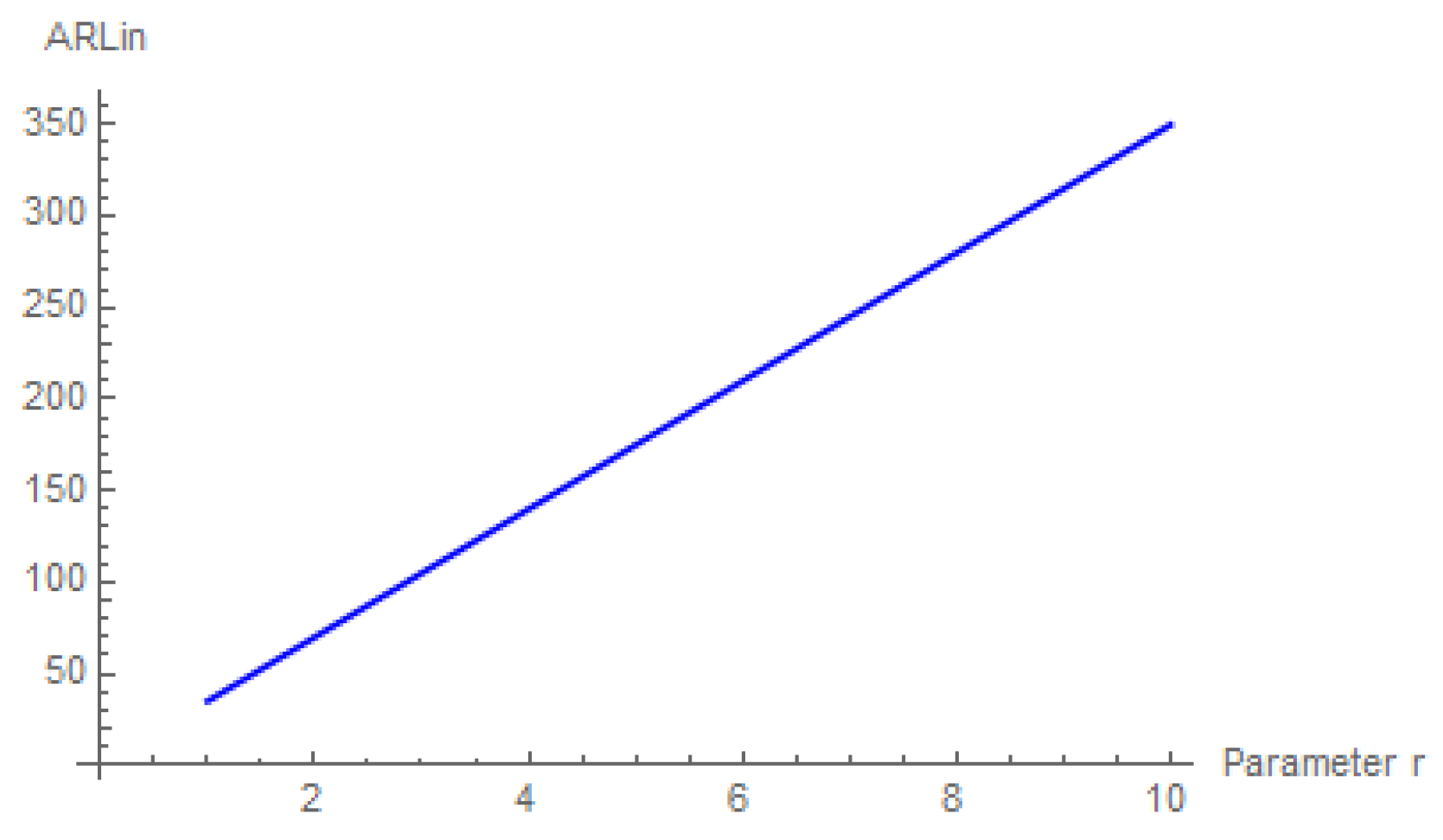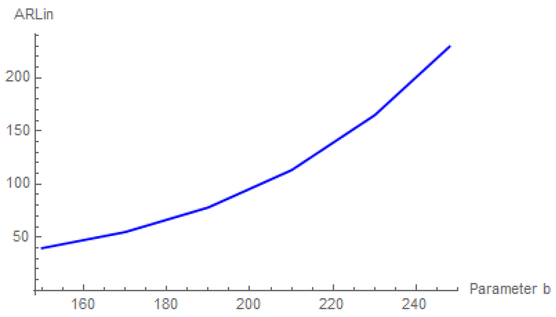Figure 1 and Figure 2 depict the behavior of the new methodology towards the sample size of the reference and the test data, respectively.

Based on Figure 1 and Figure 2, it is readily observed that, given that the remaining parameters do not vary, the in-control ARL performance deteriorates as the reference sample size increases. The same conclusion can also be drawn for the test sample size, which is utilized within the proposed framework.

As it concerns the role of parameter r, we can easily deduce that, once its value decreases, the ARL_in of the corresponding scheme becomes smaller (see Figure 3).

On the other hand, the in-control behavior of the proposed monitoring schemes worsens as the values of parameters r, i increase (see Figure 4).

In addition, the practitioner is advised to determine the values of parameters b, d to be as large as possible in order to reach a larger ARL_in. This is shown in Figure 5 and Figure 6.

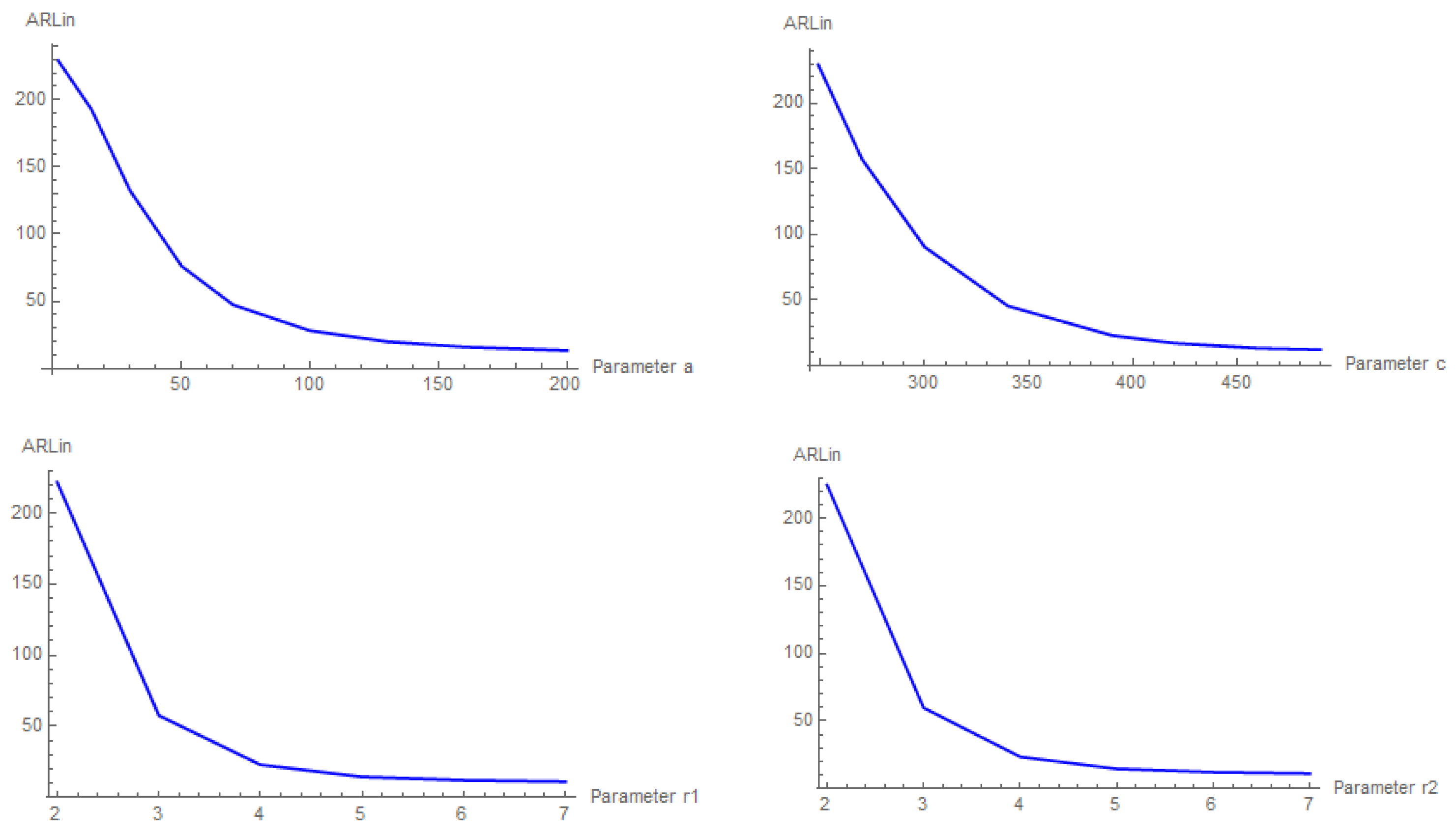
However, large values of the remaining design parameters result in small values of the in-control ARL performance of the charts. Indeed, Figure 7 offers some evidence to confirm the aforementioned conclusion.

We next compare the proposed scheme versus existing nonparametric methods. A typical approach when comparing two different control charts is to use a common in-control average run length and then to examine their out-of-control average run length. To this direction, we examine well-known nonparametric monitoring approaches and evaluate their out-of-control performance in relation to that of the proposed methods.

Table 2. ARL values of four different control charts under the N(0,1) distribution.

Shift	New Chart	W-Shewhart Chart	W-CUSUM	W-EWMA
0.0	497.23	501.92	498.64	502.94
0.25	88.17	93.12	333.45	321.52
0.50	18.35	21.88	107.19	103.15
1.00	3.44	3.46	13.04	14.29
1.50	1.33	1.33	6.25	7.52

presents a set of numerical comparisons between the newly proposed control charts and three existing distribution-free schemes. More specifically, the new chart is compared to the W-Shewhart chart, which has been introduced by [20], and the so-called W-CUSUM and W-EWMA control charts established by [21]. Note that the comparisons are made under the assumption that the underlying in-control process is normally distributed, with parameters 0 and 1.

The design parameters of all competing schemes were appropriately selected so that the corresponding rules would yield an in-control Average Run Length of approximately 500. Subsequently, the out-of-control ARL values were computed under specific mean shifts in the underlying distribution. The results in Table 2 furnish numerical support for the superior performance of the proposed monitoring schemes over existing alternatives. Indeed, the out-of-control ARL of the proposed chart is lower than that of the competing charts. In practical terms, this implies that the new charts are able to detect distributional shifts more rapidly than the alternative monitoring schemes.

As an illustration, under a distributional shift of 0.25 units, the proposed chart identifies the change within 88.17 plotting points, e.g., independent test samples, while the competing charts detect it at a noticeably slower rate. As we readily observe on the second line of the above table, the W-Shewhart chart 1 attains an out-of-control performance equal to 93.12. On the other hand, the remaining competitors achieve even worse performance. In particular, the W-CUSUM chart realizes an ARL_out equal to 333.45, while the ARL_out for the W-EWMA control chart corresponds to 321.52 plotting points.

As readily inferred from the above numerical investigation, the proposed schemes provide a competitive approach to monitoring the quality of the underlying process, regardless of the specific distribution governing it. In other words, the new control charts appear to detect potential shifts in the process distribution more quickly than their competitors in all examined cases. In addition, due to the flexibility of the proposed frameworks, which allows us to appropriately determine their design parameters in order to reach the desired level of performance under any requirements, the practitioner seems to be able to choose suitable design for every case.

4. An Illustrative Example

For illustration purposes, let us next implement the proposed monitoring framework for a real-life application. Within the present application, ocean engineers conducted 143 measurements to evaluate the performance of a breakwater structure under realistic sea conditions. The data set captures both wave height reduction—quantified as the percentage decrease in average wave height before and after the structure—and wave energy dissipation, expressed as the percentage of incoming wave energy absorbed or dissipated by the breakwater. The data set was generated as part of a pilot project implemented in collaboration with a coastal engineering consortium, focusing on the resilience of protective infrastructures in semi-exposed marine environments. Although the monitoring campaign was successfully completed and provided valuable insights regarding overtopping events, wave run-up dynamics, and structural energy dissipation, the results remain internal, serving primarily as reference material for design validation and further computational modeling.

Both variables were drawn from truncated normal distributions reflecting realistic sea conditions, using random sampling with replacement to ensure independent observations and controlled variability. Each data set included 125 observations, and the simulation was replicated 5000 times to ensure robustness and reproducibility. However, it should be noted that in the context of the present study, the data set is not analyzed to derive conclusions in the field of ocean engineering. Instead, it is employed exclusively as a demonstrative example to illustrate how the proposed methodology can be applied in practice, using real-world measurements.

The aim of this study is to provide a robust quantitative basis for optimizing breakwater dimensions and materials in future coastal protection projects. For that purpose, a monitoring framework should be developed for the crucial characteristics of the underlying structure.

Table 3. Wave height reduction (%) (upper entry) and wave energy dissipation (%) (lower entry).

72.5 91.5	76.4 79.8	77.1 77.6	73.3 83.5	78.2 85.8	72.1 73.0	78.3 94.5	80.3 90.7	79.7 73.6	82.3 76.1	77.5 80.1	81.2 84.8
77.2 82.8	73.3 84.0	79.1 81.7	80.0 75.8	75.5 91.9	77.7 73.3	78.5 73.3	80.1 71.1	82.3 83.4	73.9 90.4	84.4 86.9	79.1 75.1
81.2 81.6	75.6 91.6	77.8 81.6	73.4 74.2	77.7 82.6	82.7 85.0	80.4 75.6	80.1 89.2	81.9 89.8	84.4 75.7	80.9 91.6	82.1 77.5
77.7 76.3	70.1 87.4	77.2 67.7	73.4 87.5	75.6 91.7	79.1 75.8	76.4 88.4	73.9 75.6	77.8 86.7	72.3 73.6	71.7 73.7	79.3 74.8
87.8 85.9	76.7 79.0	72.5 77.1	75.9 87.2	84.4 84.8	74.7 83.9	79.9 74.3	75.7 86.1	72.8 77.6	81.1 85.3	73,6 90.7	79.0 71.5
76.0 87.1	77.8 85.5	80.0 88.5	78.9 76.1	72.2 77.6	78.4 85.3	88.4 68.9	88.0 70.4	78.6 74.1	87.2 78.6	84.6 79.2	80.2 82.3
79.3 84.7	82.4 81.0	84.6 80.1	80.2 73.3	85.9 77.5	81.0 76.4	84.5 68.1	84.6 72.7	82.2 79.9	82.4 84.1	88.1 74.6	80.3 80.3
80.6 81.8	88.2 70.2	81.3 77.7	85.8 82.0	77.0 69.8	83.5 78.4	82.6 73.1	81.2 70.3	82.4 79.6	91.8 84.4	80.3 80.2	80.9 68.7
88.1 82.1	81.3 75.9	82.3 71.4	73.3 79.2	87.7 70.6	85.8 81.0	82.8 73.4	86.4 77.8	89.9 83.7	90.3 76.5	90.9 74.2	92.5 78.9
91.4 80.4	85.7 82.5	71.3 78.9	87.7 70.1	80.8 83.4	76.8 79.2	86.4 72.7	92.9 68.5	90.3 80.3	90.4 74.6	92.3 77.0	91.8 81.6
85.7 73.9	75.8 70.8	82.3 69.1	81.3 78.5	79.2 80.4	91.4 74.0	91.9 77.1	80.2 82.9	92.2 81.3	82.3 85.0	81.8 72.4	86.0 79.7
75.5 70.2	85.4 70.5	83.0 70.8	82.7 74.4	85.4 76.0	90.2 77.1	92.0 79.1	90.6 81.3	89.2 82.9	87.6 83.8	88.4 88.0

displays the percentage decrease in average wave height (wave height reduction (%), hereafter), along with the corresponding percentage of incoming wave energy absorbed or dissipated by the breakwater (wave energy dissipation (%), hereafter).

Since the breakwater structure is a rubble mound one, the desirable level of wave height reduction ranges from 70% to 85%, while the corresponding one for wave energy dissipation varies from 75% to 90%.

It is evident that the first 66 measurements provide the impression that the structure performed adequately, conforming to the engineers’ requirements. Nevertheless, from 67th measurement onwards, the performance of the structure seems to be weakened, and the engineers realized that the structure does not attain a satisfactory level of performance anymore. According to the above-mentioned argumentation, measurements 1 to 66 can play the role of a reference sample of size $m=66$, while the remaining 77 measurements are test data divided into samples of size $n=11$.

We first monitor the wave height reduction (%) data. The design parameters of the suggested monitoring tool are determined such that the in-control ARL of the final control chart is determined to be almost 370. As a matter of fact, if the remaining parameters are defined as follows:

$$n=11,r=2,s=3,a=2,b=38,c=39, d=66, {i=2,j=10,r}_1=2,r_2=2$$

the constructed framework, consisting of two individual control charts, provides an in-control ARL = 368.1. The choices made previously call for the following:

• a reference sample of size $m=66 \mathrm{o}\mathrm{b}\mathrm{s}\mathrm{e}\mathrm{r}\mathrm{v}\mathrm{a}\mathrm{t}\mathrm{i}\mathrm{o}\mathrm{n}\mathrm{s}$ has been drawn when the process is in stable state;
• the ordered observations at the 2nd, 38th, 39th, and 66th position of the reference sample, e.g., the observed values $X_{2:66},X_{38:66},X_{39:66} \mathrm{a}\mathrm{n}\mathrm{d} X_{66:66}$ are related to the control limits for the resulting charts;
• test samples of size $n=11$ observations are drawn from the process;
• the quantities $Y_{i:n}^h,Y_{j:n}^h,R_1^h$ and $R_2^h$ of the monitoring statistics correspond to the h-th test sample ($h=1,2,3,4,5)$ are calculated for all available test data.

It is noteworthy that the practitioner may select any alternative combination of parameter values to develop an appropriate design that achieves the desired level of in-control performance, e.g., $AR{L}_{in}=370$. However, note that it is recommended to use a large reference sample size and a relatively small test sample size. This is justified by the fact that the first condition enables a reliable determination of the control limits, while the second facilitates the prompt detection of possible process shifts.

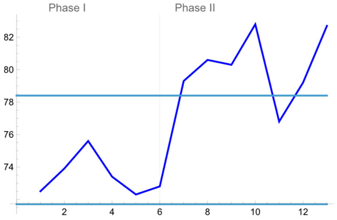
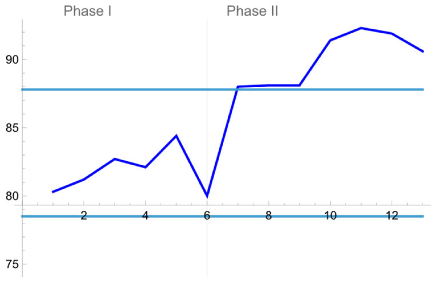
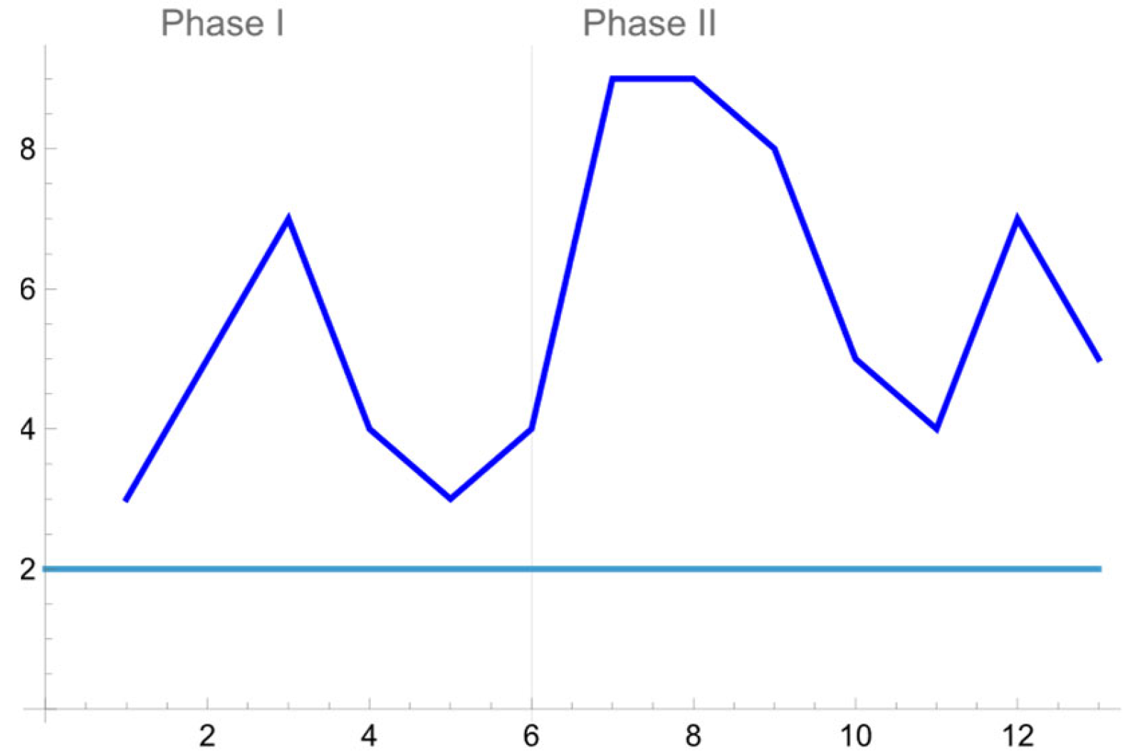
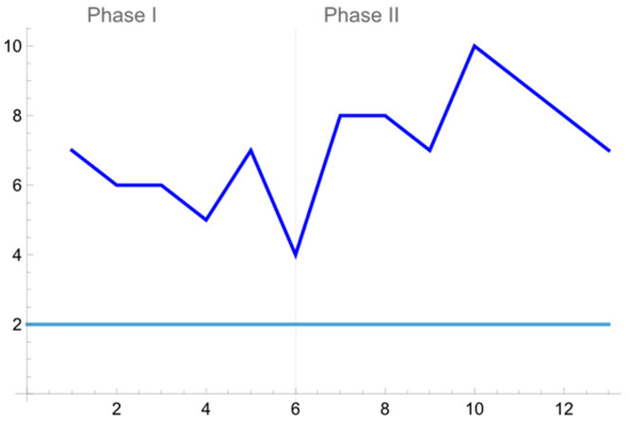
Afterwards, we construct four control charts for the wave height reduction (%) data, which comprise the proposed monitoring scheme for the available data. The results are displayed in Figure 8, Figure 9, Figure 10 and Figure 11.

The $h$ th test sample is characterized as OOC, if at least one of the following conditions is violated:

$$\begin{gathered} X_{2:66}\le Y_{2:11}^h\le X_{38:66},{ X}_{39:66}\le Y_{10:11}^h\le X_{66:66}, \\ R_1^h\ge 2\mathrm{and} R_2^h\ge 2, \end{gathered}$$

or equivalently

$$\begin{gathered} 71.7\le Y_{2:11}^h\le 78.4, 78.5\le Y_{10:11}^h\le 87.8, \\ R_1^h\ge 2\mathrm{and} R_2^h\ge 2, \end{gathered}$$

(11)

Note that every time that a plotting point is over the horizontal line, which expresses the corresponding control limit, we record a single undesirable measurement. However, under the proposed monitoring scheme, the process is characterized as OOC whenever we observe two subsequences of plotting points of length $3$ (or less), while the points contained in each one of them which lie out of control limits should be at least two in order for an OOC signal to be produced.

During Phase I, all available samples (Measurements 1 to 66 or samples 1 to 6) are not creating an OOC signal (as expected due to the good quality of the process at that time). However, the suggested distribution-free tool signals later on (Measurement 67 onwards). Indeed, an OOC (bad) signal is observed upon the 6th test data set (or 12th data set if we start to count from the beginning) since at that time two 2-out-of-3 scans are present.

Based on the above results, the ocean engineer may deduce that the underlying disruption in the performance of the structure is present, and the assembly process no longer meets their requirements. It is noticeable that the proposed scheme, which has been applied for monitoring the process, promptly detects the undesirable alteration of the process.

Furthermore, the suggested tool can also be applied for monitoring the available wave energy dissipation (%) data. More precisely, our interest focuses now on the low entries of each cell in Table 3. The first thing to do is to choose appropriate values for the design parameters of the proposed scheme, such as the in-control Average Run Length of the resulting monitoring scheme to be equal to 370 (approximately). Since we have already at hand that $m=66, n=11$, the values of the remaining parameters are suitably determined as follows:

$$n=11,r=2,s=3,a=2,b=38,c=39, d=66, {i=2,j=10,r}_1=2,r_2=2$$

The final tool, which contains two separate control schemes, achieves an in-control Average Run length which equals 368.1.

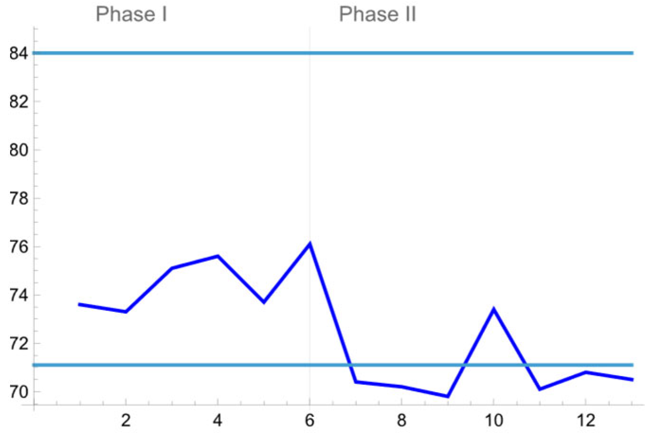
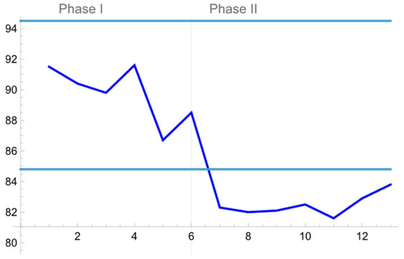
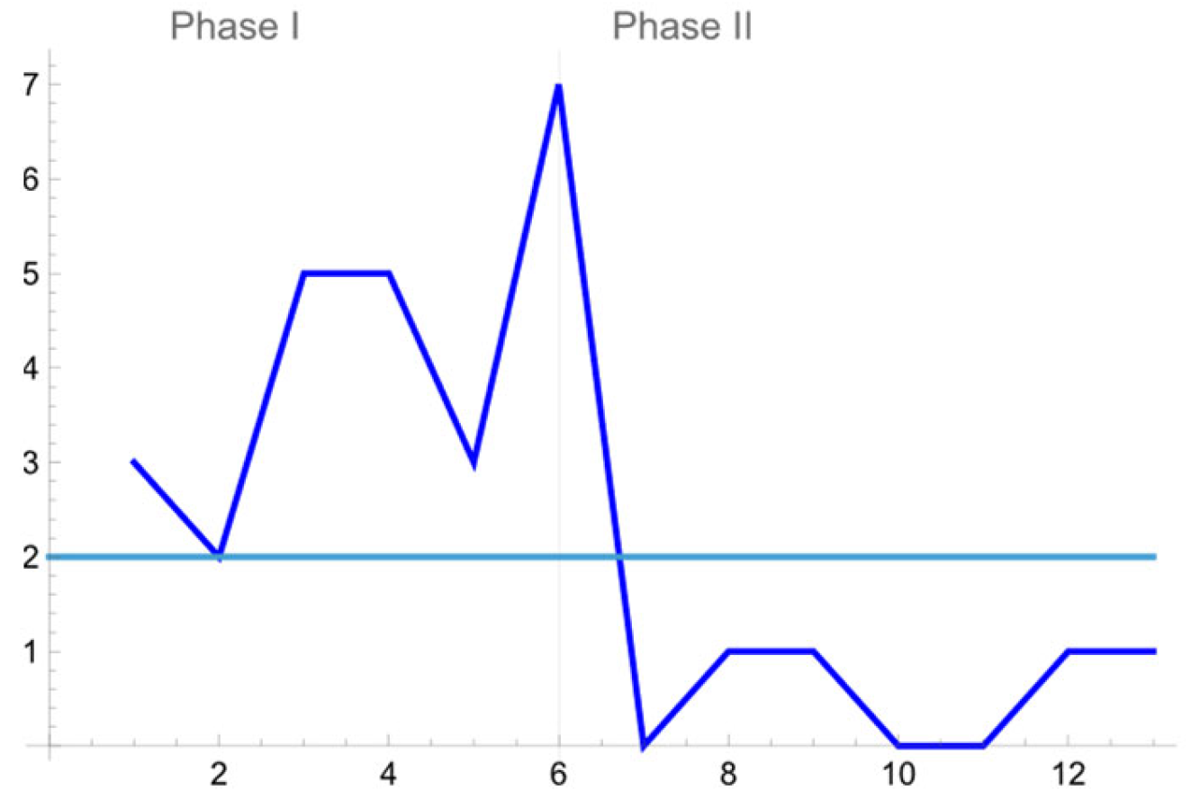
Afterwards, we construct four control charts for the wave energy dissipation (%) data, which comprise the proposed monitoring scheme for the available measurements. The outcomes are presented in Figure 12, Figure 13, Figure 14 and Figure 15.

The $h$ th test sample is characterized as OOC, if at least one of the following conditions is violated:

$$\begin{gathered} X_{2:66}\le Y_{2:11}^h\le X_{38:66},{ X}_{39:66}\le Y_{10:11}^h\le X_{66:66}, \\ R_1^h\ge 2\mathrm{and} R_2^h\ge 2, \end{gathered}$$

or equivalently

$$\begin{gathered} 71.1\le Y_{2:11}^h\le 84, 84.8\le Y_{10:11}^h\le 94.5, \\ R_1^h\ge 2\mathrm{and} R_2^h\ge 2, \end{gathered}$$

(12)

Based on Phase I and Phase II samples, the same conclusions with the ones drawn earlier for the wave height reduction (%) data, can be also stated for the available wave energy dissipation measurements.

5. Discussion

This study introduces a distribution-free monitoring tool that employs multiple scanning procedures. The scan-based rules are integrated with a distribution-free monitoring statistic, yielding promising outcomes. Furthermore, a practical application in Ocean Engineering is examined, where the proposed methodology is implemented to improve the performance of a breakwater structure. Specifically, a novel family of distribution-free Shewhart-type control charts is presented, which relies on order statistics and multiple scans. The control limits are determined by suitably selected order statistics from the reference data set, and the classification of the process as in-control or out-of-control is achieved through additional multi-scan rules. The run length behavior of these nonparametric control charts is analyzed in detail. Designers can select from the configurations listed in the manuscript tables to develop the most appropriate monitoring scheme for the application at hand. It should be mentioned that two main limitations could be met with when that practitioner attempts to apply the proposed monitoring scheme. The first one refers to the fact that quite a large reference sample is required for developing properly the corresponding control limits. The second drawback is related to the complexity of the proposed technique, since it calls for the determination of the values for a large number of design parameters. However, the latter difficulty could be considered a privilege at the same time, since it offers the practitioner the opportunity to choose the proper design among many available ones.

The paper emphasizes the potential usefulness of the proposed control charts in the field of Ocean Engineering. In terms of future potential, it could be reported that the implementation of additional or more complex scan-type rules, along with alternative distribution-free test statistics, may result in even more effective monitoring schemes. In addition, further and deeper analysis could be provided to reduce the complexity of applying the proposed technique in practice and to highlight its usefulness in other related fields as well, such as Mechanical or Industrial Engineering.