Abstract
In Bayesian statistics, the prior distributions play a key role in the inference, and there are procedures for finding prior distributions. An important problem is that these procedures often lead to improper prior distributions that cannot be normalized to probability measures. Such improper prior distributions lead to technical problems, in that certain calculations are only fully justified in the literature for probability measures or perhaps for finite measures. Recently, expectation measures were introduced as an alternative to probability measures as a foundation for a theory of uncertainty. Using expectation theory and point processes, it is possible to give a probabilistic interpretation of an improper prior distribution. This will provide us with a rigid formalism for calculating posterior distributions in cases where the prior distributions are not proper without relying on approximation arguments.
Keywords:
Bayesian statistics; expectation measure; improper prior distribution; expected value; point process; Poisson point process; s-finite measure; posterior distribution; statistical model; stopping time MSC:
60A05; 60G55
1. Introduction
In Bayesian statistics, we usually use probability measures to quantify uncertainty. These probability measures are defined as measures with total mass equal to 1. Before we do any calculations, we need a prior distribution, so we need guidelines about how such prior distributions should be assigned to a specific problem. A subjective Bayesian would have consistency as the only limitation on how prior distributions are assigned. A significant problem with this approach is that it is subjective, so that more or less any conclusion can be reached by a suitable choice of prior distribution. On the contrary, an “objective” Bayesian would advocate for specific methods for determining prior distributions in particular situations. Although such methods may not be objective in any absolute sense, the aim should be that the methods are intersubjective in the sense that different scientists would get the same prior distribution if they agree that certain conditions are fulfilled.
Objective Bayesians have developed different methods for assigning prior distributions, and a significant problem is that these methods often lead to improper prior distributions, where the prior distributions are described by measures that have infinite mass so that they cannot be normalized. Although posterior distributions can often be calculated from such improper prior distributions by plugging into a formula, the formula is not well justified in the usual probabilistic models of uncertainty. Handling and interpreting improper prior distributions is a significant problem in the Bayesian approach to statistics [1], and this will be the primary focus of the present paper.
In many textbooks, improper prior distributions are handled by the selection of a “large” subset of the parameter space. If the parameter space is and the improper prior measure is , then one selects a subset , such that . Then, the measure restricted to is normalized, so that the normalized measure can be interpreted as a probability measure. If is an increasing sequence of sets, such that , then the posterior based on the normalized version of the measure restricted to will converge to the posterior based on . Hence, by selecting a sufficiently large subset of the parameter space, we get a probabilistic inference that approximately gives the right result. Akaike and many others have advocated this approach to handling improper prior distributions [2]. See [3] for a more recent exposition regarding the approximation of improper priors by probability measures.
Inference based on restriction of the parameter space is problematic for two reasons. The first reason is that the subset should, in principle, be chosen before any observation has been made, and if is improper and , there will exist observations for which the posterior based on is very different from the posterior based on the whole parameter space . The second reason is that if is chosen with a finite measure, it will often conflict with how we justify the use of the prior measure . If, for instance, is determined as a Haar measure on a non-compact group, then the restriction of to a set of finite measure will, in general, not be a Haar measure.
1.1. Expectation Theory
In a recent paper, expectation theory was presented as an alternative to the Kolmogorov style of probability theory [4]. Our main result is that with expectation measures at our disposal, we can handle improper prior distributions without restricting to a subset of the parameter space. No approximation argument is required as long as we condition on an event of positive finite measure. Approximation may be relevant if we condition on an event of measure 0, but this problem is related to using continuous measures and not to the prior distribution being improper.
In [4], it was shortly mentioned that expectation theory allows us to give a probabilistic interpretation for improper prior distributions and conditioning based on such measures. Here, we will provide a more detailed exposition on this problem. Some results in [4] will be generalized from discrete measures to s-finite measures.
The basic objects for describing uncertainty in expectation theory are s-finite measures rather than probability measures that are the fundamental objects in Kolmogorov-style probability theory. These measures can be interpreted as expectation measures of specific point processes. This gives a probabilistic interpretation of expectation theory, so there is no dichotomy between probability theory and expectation theory, but the focus is slightly different in expectation theory. Expectation theory and Kolmogorov-style probability theory are two theories that both quantify uncertainty, and each of the two theories comes with a set of basic concepts, as illustrated in Table 1.

Table 1.
Fundamental concepts in Kolmogov-style probability theory and the corresponding fundamental concepts in expectation theory.
Recently, M. Albert and S. Mellick have proved that if a group is locally compact, second-countable, unimodular, non-discrete, and non-compact, then any free-probability-measure-preserving action of the group can be realized by an invariant point process [5,6]. As we will see in this paper, the idea of interpreting measures that are not probability measures via point processes can be used for any s-finite measure without reference to a group structure. Since the methods and results of M. Albert and S. Mellick are so closely related to the present work, we will briefly mention how Haar measures are relevant for determining prior distributions in Section 2.7.
It is possible to define a monad for point processes [7]. The monad defined in [7] is also related to the observation that the Giry monad is distributive over the multiset monad, as discussed in [8]. These results from category theory provide the underlying structure that allows for the results presented in this paper.
1.2. Terminology and Notation
In principle, there is no dichotomy between expectation theory and Kolmogorov-style probability theory, but in practice, we have to make some modifications to the terminology in order to avoid confusion.
In standard probability theory, a probability measure lives in either the sample space [9] (p. 292), [10] (Section 1.3), [11] (p. 22), the outcome space [12] (p. 10), [13] (Sec. 1.1), the space of elementary events [14] (p. 5), the sample description space [15] (p. 7), or the possibility space [16] (p. 3). In this paper, we will use the term outcome space, and the elements of the outcome space will be called outcomes, points, or letters. The word sample will be used informally about the result of sampling. Sampling can often be modeled by a point process where the result is a multiset, i.e., a set of points in the outcome space each with a weight indicating the number of observations of that point. The result of a point process will be called an instance of the point process, and the elements of the instance will often be called points. We avoid the term sample space, because it may make it less clear whether a sample leads to a point in outcome space or whether it leads to a multiset over the outcome space.
If is a probability measure, then the conditional probability measure given a measurable set A is denoted as . In the standard approach to probability theory, the conditional probability measure may be viewed as a restriction of the original probability measure to a subset. In many expositions, the measure restricted to a measurable set A is denoted as [17] (Sec. 3) or [18] (p. 3). In expectation theory, the restricted measure and the conditional measure are two related but distinct measures, which should not be confused. For this reason, we will denote the restricted measure as .
A measure with a total mass of 1 is usually called a probability measure. We will deviate from this terminology and use the alternative term normalized measure for a measure with total mass 1 [12] (p. 10). We will reserve the word probability measure to situations where the weights of a normalized measure are used to quantify uncertainty, and it is known that precisely one observation will be made, and one can decide which event the observation belongs to in a system of mutually exclusive events that cover the whole outcome space. Similarly, we will talk about an expectation measure if our interpretation of its values is given in terms of expected values of some random variables, or if it is the expectation measure of a point process.
If a measure is used to quantify our prior knowledge about a parameter before observation, we will call it a prior distribution. Following [19], we use the term proper prior when the measure is normalized, and in other cases, we say that the prior distribution is improper. Note that many statisticians only use the term improper prior when the measure has infinite total mass [20] (Chap. 8.2 Improper prior).
1.3. Organization of the Paper
In order to make this paper more self-contained, there is some slight overlap between this paper and [4], but the reader should consult [4] if the reader is interested in a more complete motivation for basing a theory of uncertainty on expectation measures rather than probability measures.
In Section 2, we provide a brief introduction to expectation theory and related topics concerning point processes. We also discuss statistical models and some methods for calculating prior distributions. There are many other ways to get prior distributions, and this is not an attempt to cover this topic. We just provide enough background material to present some examples of statistical models with prior distribution.
Section 3 contains the main contribution of this paper. We provide a probabilistic interpretation of improper priors based on point processes. The interpretation allows for the calculation of posterior distributions without relying on any approximation arguments.
We end the paper with a short discussion.
2. Methods
Here, we will introduce the concepts and results needed in the subsequent sections. For motivation and more details, we refer to the literature.
2.1. Observations and Expectations
In statistics, data are often given in terms of frequency tables. To each entry, the table gives the observed frequency of that entry. An example of such a frequency table is Table 2.
Table 2.
Frequencies of eyes in 68 independent throws with a six-sided die.
A frequency table can be identified with a multiset, i.e., a set where each point has a multiplicity. To relate such multisets to Kolmogorov-style probability theory, we will represent them as measures. Let denote a measurable space. Observations in will be represented as finite or countable sums of Dirac measures.
Example 1.
The frequencies in Table 2 can be represented by the measure
A finite or countable sum of Dirac measures will be called an observation measure. One can define kernels with expectation measures as outcomes, and such kernels can be composed in the same way as Markov kernels can be composed. The category of finite expectation measures was studied in [4], and this category may serve as a model of descriptive statistics.
2.2. Expectations as s-Finite Measures
Before making any observations, there will be uncertainty about what the observations will be. The uncertainty will be quantified in terms of an expectation measure, which is a measure on an outcome space , such that for the value is the expected value of the number of observations in B. If we would allow all measures as expectation measures, we would get into technical problems. For instance, Tonelli’s theorem does not hold for arbitrary measures, and kernels based on arbitrary measures cannot be composed. For this reason, we should look for a well-behaved category that can handle both normalized measures and observation measures.
The set of normalized measures on will be denoted or for short. Like Rényi, we are more interested in kernels than in measures [21,22,23]. A measurable mapping is called a Markov kernel, and an important property of Markov kernels is that they can be composed. Let and denote Markov kernels from to and from to , respectively. The two Markov kernels can be composed by
With this compostion, the measurable spaces and Markov kernels form a category that Lawvere was the first to study [24]. From the point of view of category theory, the composition is related to the fact that the functor is part of a monad [4,25].
A kernel is said to be a sub-Markov kernel if for all [26] (Def.1, ii’). Sub-Markov kernels can be composed in just the same way as Markov kernels. Thus, the measurable spaces and sub-Markov kernels form a category with the category of Markov kernels as a sub-category.
A kernel is said to be s-finite if there exists a countable set of sub-Markov kernels , such that . Such s-finite kernels can be composed, resulting in an s-finite kernel [27]. To see that, let be a s-finite kernel from X to Y and let be a s-finite kernel from X to Y. Then
which is clearly an s-finite kernel. With this composition, we get a category of s-finite kernels, and the category of Markov kernels is a sub-category.
Many textbooks on probability theory or general measure theory focus on -finite measures. The problem is that the composition of -finite kernels may lead to s-finite kernels that are not -finite. In recent years, s-finite measures have gained increasing attention among people studying denotational semantics for probabilistic programming [23,27,28,29].
2.3. Point Processes
We will define a point process with points in the measurable space . In the literature on point processes, will be a d-dimensional Euclidean space, but we will not make such a restriction. Let denote a probability space. A transition kernel from to is called a point process if
- For all , the function is a s-finite measure.
- For all bounded sets , the random variable is a count variable.
In the literature, it is often assumed that that is locally finite rather than s-finite, but we will make no such restriction. For further details about point processes, see [30] or [31] (Chapter 3).
The interpretation is that if the outcome is , then is a measure that counts how many points there are in various subsets of , i.e., is the number of points in the set . Each measure will be called an instance of the point process. We note that under weak topological conditions, an instance of a point process is the same as an empirical measure. In the literature on point processes, one is often interested in simple point processes, where when B is a singleton. However, point processes that are not simple are also crucial for the problems that will be discussed in this paper.
The definition of a point process follows the general structure of probability theory, where everything is based on a single underlying probability space. This will ensure consistency, but often this probability space has to be quite large if several point processes or many random variables are considered simultaneously.
The measure is called the expectation measure of the process if for any we have
The term intensity measure is sometimes used instead of expectation measure. For simple point processes, expectation measures are often expressed in terms of the Radon–Nikodym derivative with respect to an underlying measure. In such cases, the term intensity measure is appropriate. However, we also consider point processes that are not simple, so we prefer the term expectation measure.
The expectation measure gives the mean value of the number of points in the set B. Different point processes may have the same expectation measure. A one-point process is a process that outputs precisely one point with probability 1. For a one-point process, the expectation measure of the process is simply a probability measure on . Thus, probability measures can be identified with one-point processes.
2.4. Poisson Distributions and Poisson Point Processes
For , the Poisson distribution is the probability distribution on with point probabilities:
For , we define as the normalized measure concentrated on ∞.
It was proven in [32] (Thm. 3.6) that for any s-finite measure on , there exists a point process , such that
- For all , the random variable is Poisson distributed with a mean value .
- If and are disjoint, then the random variables and are independent.
Such a process is called a Poisson point process with expectation measure , and we will denote it by . All results regarding an s-finite measure can now be translated into results regarding the Poisson process . We call this the Poisson interpretation of the measure.
Example 2
(Temporal Poisson process). Let denote the Lebesgue measure restricted to the interval . Then, is a homogeneous Poisson process with intensity 1. This is normally considered a temporal model, where the elements in are considered as times where certain events happen.
Example 3
(Spatio-temporal Poisson process). If is a Poisson point process with points in space, then can be viewed as a spatio-temporal point process, where any points of the spatial process are created at a random time in . This process has the process as its marginal distribution.
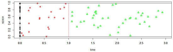
Formally, one may consider the spatio-temporal Poisson process where points continue to be created. An instance of such a process would have infinitely many points, so it cannot be simulated. A simulation of a spatio-temporal process can be found in Figure 1.
Figure 1.
Simulation for some point processes. The black points are points in an instance of a Poisson point process on distributed according to a uniform distribution. The red point are point in an instance of a spatio-temporal process, where one has assigned a random time in to each of the black points. The green triangles illustrate a continuation of the same process from time 1 to time 3. One cannot simulate the whole spatio-temporal with time in because the expected number of points is infinite.
2.5. Measures and Kernels Associated with Statistical Models
Let be a measurable space that represents the possible outcomes. Further, let be a measurable space that represents possible values of a parameter of a statistical model. A statistical model is given by a Markov kernel that assigns a probability measure on to each parameter [33]. The goal of the statistician is to make an inference on the unobserved value of based on an observed value .
Assume that our prior knowledge about the parameter is given by the measure on . This leads to a joint measure on . Following [26], the joint measure will denote . For and , we have a measurable function from , which is given by . The joint measure is defined by
Let denote the marginal measure of on , i.e., is the restriction of to the sub-algebra of consisting of sets of the form . If is a -finite measure, then there exists a Markov kernel from to , such that
and we will write for short. Remark that, at this level, the existence of the Markov kernel is a purely formal construction.
In information theory, a Markov kernel is called an information channel with input alphabet and output alphabet [34] (Chapter 8). In the branch of information theory called channel coding, the input letters are controlled by the sender (Alice), but unknown to the receiver (Bob). The goal of Bob is to make an inference about the letter sent by Alice based on the letter received by Bob.
A Markov kernel can be used to model sequences of observations in in two ways. In statistics, a sequence of length n is modeled by , which gives a Markov kernel from to . In channel coding, a sequence of length n is modeled by . In channel coding, we get a Markov kernel from to .
2.6. Minimax Redundancy and Jeffreys’ Prior
Prior distributions play a major role in Bayesian statistics. We will provide examples of how prior distributions are calculated using ideas from information theory. The information-theoretic approach to calculating prior distributions will also lead to a motivation using Jeffreys’ prior. The examples we discuss in this section will be used in subsequent sections. A detailed discussion about different methods for the calculation of prior distributions is beyond the topic of this article. We will refer to [35] for a review of the subject, including a long list of references.
One method for calculating a prior distribution for a statistical model is to consider the model as an information channel. Here, we will only mention some of the basic ideas briefly. The reader may consult [36] or [37] for a more detailed exposition. Assume for simplicity that is a finite set. If data is distributed according to , then the code that will give the shortest mean code-length uses a code-word of length proportional to when the letter b is encoded. Optimal coding requires that is known. If is not known and the data is coded as if the distribution was given by the probability measure P, then the code-length of the code-word corresponding to the letter b is . If the letter is b, the redundancy of coding as if the distribution was given by P when it is actually is defined as the difference in code-length., i.e.,
The mean value of the redundancy (8) is given by the Kullback–Leibler divergence is defined by
The Kullback–Leibler divergence quantifies redundancy, i.e., the mean number of bits one can save by coding according to the true distribution rather than coding as if the data were distributed according to P. The minimax redundancy is given by
where the minimum in Equation (10) takes over all probability measures P on . Coding according to the distribution P that minimizes the maximal redundancy is optimal, in the sense that it leads to the shortest description of data compared with what could have been achieved knowing the true distribution .
The capacity of the channel is the maximal transmission rate, which is the maximal mutual information between input and output [34] (Chap. 8). According to the Gallager–Ryabko Theorem [38], the maximal transmission rate equals the minimax redundancy. If is the distribution that achieves the minimum in Equation (10), then a capacity-achieving input distribution is the same as a probability measure Q, such that
The input distribution Q is the optimal prior distribution if we want to minimize the maximal redundancy.
Example 4
(The binary erasure channel). The binary erasure channel has an input alphabet and an output alphabet A Markov kernel is given by
The output letter e represents an erasure of the input letter. The capacity achieving input distribution is the uniform distribution on the input alphabet . See [34] (Subsec. 8.1.5) for a detailed discussion of the binary erasure channel.
Example 5
(The binomial model). The binomial distributions form a statistical model with point probabilities . In this case, there is no unique capacity-achieving distribution if the parameter space is . If we restrict the parameter space to the set of possible maximum likelihood estimates , there is a unique capacity-achieving distribution that can be used as a prior distribution on Θ. For small values of n, the exact optimal distribution can be calculated. If, for instance , the optimal distribution on is . In general, no closed formula for the capacity-achieving distribution exists, but it can be approximated using an iterative algorithm (see [36] (Sec. 5.2) and [39]).
Kullback–Leibler divergence given by Equation (9) equals the Rényi divergence of order 1. If we use the Rényi divergence of order ∞ [40] (Thm. 6)
instead of Kullback–Leibler divergence, then we get the regret, which reveals how many bits can be saved by coding with respect to P rather than coding according the model Q for the data that is least favorable without any assumption on how the data sequence is generated. From a statistical perspective, an analysis based on regret rather than redundancy is more conservative.
Example 6
(The binomial model). The distribution that achieves minimax regret can be calculated as the normalized maximum likelihood (NML) distribution. It has point probabilities
This corresponds to the prior on the parameters .
As demonstrated in Examples 5 and 6, finding a prior using minimax redundancy or minimax regret will, in general, lead to different results, but for long data sequences, the distributions that achieve minimax redundancy and minimax regret, respectively, can both be approximated by Jeffreys’ prior [37] (Sec. 8.2). Thus, Jeffreys’ prior can be used as an approximation of the prior that is optimal in the sense of achieving minimax redundancy or minimax regret.
Let denote a statistical model and assume that for some dominating measure . Assume further that is an open subset of , and that is twice differentiable. Note that this excludes statistical models where is a discrete set. The Fisher information matrix is given by
Jeffreys’ prior is defined as the distribution on with density
One should note that there are other reasons for choosing Jeffreys’ prior than the ones based on information theory. For instance, except for a constant factor, Jeffreys’ prior does not depend on parametrization [41,42].
Example 7
(The binomial model). For the binomial model, we have
The Fisher information equals the mean value of (17):
Jeffreys’ prior has density proportional to
In this case, Jeffreys’ prior has finite mass so that it can be normalized. The normalized Jeffreys’ prior is a beta distribution with parameters . The posterior distribution of p, if x successes and failures have been observed, is a beta distribution with parameters .
Example 8
(The exponential model). For , the exponential distribution has density:
We have
Hence, the Fisher information is given by
and Jeffreys’ prior has density . In this case, Jeffreys’ prior is improper, and it cannot be normalized. This is related to the fact that the statistical model has infinite channel capacity. Jeffreys’ prior is also optimal in an information-theoretic sense without relying on any approximation argument involving long sequences [43,44].
With this prior measure, the joint measure has density . The marginal measure of X is
The conditional distribution of the parameter Λ, given , is an inverse gamma distribution with density , shape parameter 1, and scale parameter x.
Example 9
(The Poisson model). For the Poisson model with , we have
Therefore, the Fisher information equals
Therefore, Jeffreys’ prior has density on , which cannot be normalized.
The marginal measure on X is . The conditional distribution of the parameter as a random variable Λ given has the following density:
where the parameter Λ is gamma distributed with scale parameter 1 and shape parameter .
2.7. Haar Measures
Many statistical models have symmetries, and these can be useful in determining prior distributions. Let denote a statistical model with outcome space . Let G be a group that acts on both and via and . The group action is said to be covariant if
The notion of covariance was introduced by A. Holevo in the context of quantum information theory [45]. Group actions on statistical models have also been discussed in the statistical literature (see [33] (p. 1241)) and references in that paper), but the idea is less used and developed in statistics than in quantum information theory. Equation (27) can be expressed in terms of the following commutative diagram
If a group has a covariant action on a statistical model, then, one may argue, the prior should be invariant under the action of the group.
Theorem 1
(Existence of Haar measures [46,47]). Let denote a locally compact group. Then, there exists a measure μ that is invariant under left actions, i.e., for any measurable set and any we have The measure μ is unique except for a multiplicative constant.
A left invariant measure is called a left Haar measure. The left Haar measure is finite if, and only if, the group is compact. A locally compact group also has a right Haar measure that may be different from the left Haar measures, but if the group acts on a set X from the left, we are mainly interested in the left Haar measures. On abelian groups, discrete groups, and compact groups, all left Haar measures are also right Haar measures. For such groups, we do not need to distinguish between left Haar measures and right Haar measures and just talk about Haar measures [48].
If a group has a left action on the parameter space, and the action is transitive, then the action induces a measure on the parameter space, which is invariant under actions of the group. This measure will be the uniquely determined left invariant measure, except for a multiplicative constant.
Example 10
(Binary erasure channel). For the binary erasure channel, there is a symmetry between the letters a and b, and this symmetry holds both for the input alphabet and for the output alphabet . Measures that put equal weight on a and b are the only measures on that are invariant under the symmetry. The symmetry does not depend on whether we use minimax redundancy or minimax regret as a criterion for selecting the prior, so these and many other criteria for selecting a prior all lead to the same prior except perhaps for a multiplicative constant.
If the outcome space is discrete and the parameter space is continuous, then a covariant action of a symmetry group cannot be transitive on the parameter space.
Example 11
(The Binomial model). In the binomial model, there is a symmetry between success and failure corresponding to the mapping in the parameter space. The prior distributions in Examples 5–7 are all symmetric, but the action of the symmetry group is not transitive, so symmetry alone does not determine the prior.
Example 12
(The exponential model). For the exponential model , the group of positive numbers with multiplication has a covariant action on the statistical model via scaling . A measure with density with respect to the Lebesgue measure is a Haar measure on . Therefore, Jeffreys’ prior must be proportional to the Haar measure.
If a group is locally compact and -compact, then any left Haar measure is s-finite, and there exists a Poisson point process with the Haar measure as the expectation measure. This gives a probabilistic interpretation that will allow for a much wider use of Haar measures in probability theory.
3. Results
Many textbooks handle improper prior distributions by restricting the parameter space. In this section, we will utilize expectation theory to provide a more satisfactory approach to handling improper prior distributions.
3.1. Normalization and Conditioning for Expectation Measures
Empirical measures can be added, restrictions can be taken, and induced measures can be found. Using the same formulas, these operations can be performed on expectation measures, but we are not only interested in the formulas but also in probabilistic interpretations.
The norm of a (positive) measure is defined by , and the normalized measure has an interpretation as a probability measure, which is equivalent to a one-point process.
The following proposition gives a probabilistic interpretation of restriction for expectation measures via the same operations applied to empirical measures. A simple calculation proves the proposition.
Proposition 1.
Let be a probability space. Let denote a point process with expectation measure μ and with points in . Let B be a subset of . Then
Normalized measures are usually called probability measures, and the next theorem gives a probabilistic interpretation of the normalized measure by specifying an event that has probability equal to .
Theorem 2
([4] (Thm. 10)). Let B be a measurable subset of . Let μ be a non-trivial finite measure on . If P denotes a probability measure on Ω and is a Poisson point process with expectation measure μ, then
Proposition 1 holds for all point processes, but in Theorem 2, it is required that the point process is a Poisson point process. An example of a point process where Equation (30) does not hold can be found in [4] (Ex. 5).
Theorem 2 states that is the probability of observing a point in B, which has an interpretation that involves two steps.
- 1.
- Observe a multiset of points as an instance of a point process.
- 2.
- Select a random point from the observed multiset.
By replacing the point process by a spatio-temporal point process we can replace this two-step interpretation by a one-step interpretation. The one-step interpretation will be formulated as a theorem that has a much simpler proof than the proof of Theorem 2 given in [4], and the proof of the new theorem will not rely on the proof of Theorem 2.
Consider the point process on . From this process, we construct a spatio-temporal process. To each point in an instance of the point process , we randomly select a number in according to a uniform distribution. The number selected for a specific point is considered as the time at which the point is created. This gives the process . Instead of choosing a random point from the instance of the original point process , we choose the first point in the spatio-temporal point process.
For the process , there is a risk that no point is created before time . To avoid this problem, we replace the process by the process with points in . Let T be the time at which the first point is created. Then, T is a stopping time. The distribution of the point created at time T will be .
We can summarize this result in the following theorem:
Theorem 3.
Let B be a measurable subset of . Let μ be a non-trivial finite measure on . Let P denote a probability measure on Ω and let be a spatio-temporal Poisson process with expectation measure on . For an instance of the process, let denote the point in the instance, for which t has the smallest value. Then
Proof.
Let S denote the waiting time until the first point in B has been observed, and let T denote the waiting time until the first point in has been observed. The S has an exponential distribution with mean , and T has an exponential distribution with mean . We have
which proves the theorem because □
A simulation illustrating the theorem is given in Figure 2.
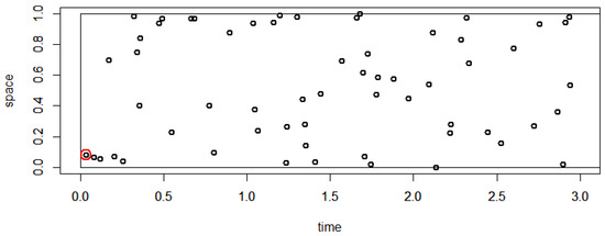
Figure 2.
Simulation of a spatio-temporal based on a measure proportional to the beta distribution with and . A red circle marks the first point in the instance. The process is stopped at time equal to 3, but it could have been stopped at any time after the first point has been observed.
3.2. Conditioning for Improrer Prior Measures
Here, we shall look at how the results of Section 3.1 will allow us to give an exact interpretation of conditional probabilities with respect to an improper prior distribution. First, we note that the Poisson interpretation of normalized expectation measures carries over to conditional measures.
Theorem 4.
Let B be a measurable subset of . Let μ be an s-finite measure on . Let P denote a probability measure on Ω and let be a spatio-temporal Poisson process with expectation measure on . Assume that A is a measurable subset of such that . For an instance of the process let denote the point in the instance for which t has the smallest value. Then
Proof.
A conditional measure is the normalization of an expectation measure restricted to a subset.
The corollary is proved by applying Theorem 2 to the measure . □
Theorem 4 is illustrated in Figure 3.
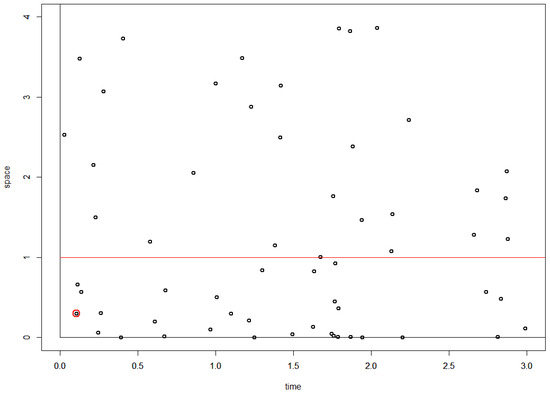
Figure 3.
Simulation of a spatio-temporal process based on an un-normalized measure with density proportional to . We condition on (indicated by the red line), which has finite measure. A red circle marks the first point in the instance below the red line. The process was stopped at time equal to 3, but it could have been stopped at any time after the marked point had been observed. Note that if we do not restrict to , then the marked point is not the first point. Only values of were included in this simulation, but all points with are irrelevant, for which point we should mark as the first point satisfying .
With this result at hand, we get an interpretation of posterior distributions calculated based on improper prior distributions.
Example 13
(The binary erasure channel). Consider the binary erasure channel discussed in Example 4. The prior measure μ gives the expected number of input letters from the alphabet . We run a spatio-temporal Poisson process on . This will give a stream of input letters at a rate of per time unit. Using the Markov kernel , we get a spatio-temporal process on .
For any instance of this process, we look at the first output letter that equals e. For this first instance, we look at the corresponding input letter. The probability of the input letter a is , and, similarly, the probability of the input letter b is . Thus, the conditional probability distribution over input letters, given the output letter e, equals the probability that an instance with output letter e has a certain input letter.
Example 14
(The binomial model). In this example, the parameter space is the . If we fix the number n of output letters generated by a single value of the parameter and calculate the prior distribution that maximizes the transmission rate or, equivalently, minimizes the maximal redundancy, then the prior is concentrated on a finite subset of the parameter space. The prior will have a finite total mass, and it can be normalized to a probability measure. If the measure is not normalized, we will get a probabilistic interpretation by running a spatio-temporal process in exactly the same way as in the previous example.
If we use Jeffreys’ prior, which is a good approximation to the case where n is large, then it is still possible to normalize the prior measure. Normalizing the measure corresponds to selecting the first point in a point process. The posterior distribution of the parameter given the output letters equals the distribution of the parameter, given that the first point (input value of the parameter) in the spatio-temporal process leads to these output letters.
Example 15
(The Poisson model). For this model, Jeffreys’ prior cannot be normalized. An instance of the point process with Jeffreys’ prior as expectation measure has infinitely many points with probability 1. The same is true for the joint distribution of Λ and X. Therefore, the corresponding spatio-temporal process has no first point. This may appear as a problem, but if the joint distribution is restricted to then the measure is finite and an instance of the corresponding spatio-temporal process will have a first point. The distribution of this first point will be the conditional distribution of Λ given , i.e., a gamma distribution with scale parameter 1 and shape parameter .
In Example 15 one may object that it is not realistic to observe an instance of a point process with infinitely many points. For instance, a computer simulation will never be able to output infinitely many points. Although it is not possible to observe infinitely many points, this is irrelevant for our result because we are only interested in what happens under the condition . What happens outside this event is irrelevant.
Example 16
(The exponential model). It is not possible to normalize Jeffreys’ prior for the family of exponential distributions. Therefore, one cannot run the corresponding spatio-temporal process and take the first point because in any small time interval, there will be infinitely many points. If, instead, we have a certain interval for the output variable with finite mass, then we can take the first point in the process that lies in this interval. The conditional distribution of the parameter is a mixture of conditional distributions given the numbers in the interval weighted and normalized according to density on the interval.
If the interval is short, then the conditional distribution given any point in the interval will be approximately constant, and conditioning on the interval will be approximately the same as conditioning on a point.
In the exponential model, one has to use some approximation argument if one has to condition with respect to the random variable having an exact value rather than being an element of an interval. This problem has nothing to do with the prior being proper or not. We will run into this problem for any continuous model, even if the parameter space is a finite set.
4. Discussion
We have applied expectation theory to give a probabilistic interpretation of improper prior distributions via the Poisson interpretation. This led to a probabilistic interpretation of conditioning with respect to improper prior distributions. With a probabilistic interpretation of improper prior measures and conditioning in place, one should go through all the arguments in favor of using specific methods for calculating prior distributions. We have briefly discussed Haar measures and Jeffreys’ prior, but a careful review of all the methods is needed, which is beyond the scope of this paper.
In this paper, a statistical model was identified with a Markov kernel, as is usually done in statistics. From the point of view of expectation theory, it would be more natural to identify statistical models as s-finite kernels rather than Markov kernels. This would not make much of a difference regarding the handling of improper distributions with respect to conditioning. The idea of basing statistics on more general kernels than Markov kernels has also been promoted recently by Taraldsen et al. [49].
In [50,51], it was proven that for one-dimensional exponential families, minimax redundancy is finite if, and only if, minimax regret is finite. It was also demonstrated that a similar result does not hold for three-dimensional exponential families. There are still no results that relate the finiteness of minimax redundancy or minimax regret with the finiteness of Jeffreys’ prior, and there are still a lot of open questions regarding improper prior distributions.
Funding
This research received no external funding.
Data Availability Statement
No new data were created or analyzed in this study. Data sharing does not apply to this article.
Acknowledgments
I want to thank Peter Grünwald and Tyron Lardy for stimulating discussions related to this topic.
Conflicts of Interest
The author declares no conflicts of interest.
References
- Jones, A. Improper Priors. Available online: https://andrewcharlesjones.github.io/journal/improper-priors.html (accessed on 29 August 2025).
- Akaike, H. The interpretation of improper prior distributions as limits of data dependent proper prior distributions. J. R. Stat. Soc. 1980, 42, 46–52. [Google Scholar] [CrossRef]
- Bioche, C.; Druilhet, P. Approximation of improper priors. Bernoulli 2016, 22, 1709–1728. [Google Scholar] [CrossRef][Green Version]
- Harremoës, P. Probability via Expectation Measures. Entropy 2025, 27, 102. [Google Scholar] [CrossRef]
- Mellick, S. Point Processes on Locally Compact Groups and Their Cost. Ph.D. Thesis, Alfréd Rényi Institute of Mathematics, Budapest, Hungary, 2019. [Google Scholar]
- Abért, M.; Mellick, S. Point processes, cost, and the growth of rank in locally compact groups. Isr. J. Math. 2022, 251, 48–155. [Google Scholar] [CrossRef]
- Dash, S.; Staton, S. A Monad for Probabilistic Point Processes. arXiv 2021, arXiv:2101.10479. [Google Scholar] [CrossRef]
- Jacobs, B. From Multisets over Distributions to Distributions over Multisets. In Proceedings of the 36th Annual ACM/IEEE Symposium on Logic in Computer Science, New York, NY, USA, 29 June–2 July 2021; LICS’21. pp. 1–13. [Google Scholar] [CrossRef]
- Everitt, B.S. The Cambridge Dictionary of Statistics; Cambridge University Press: Cambridge, UK, 1998. [Google Scholar]
- Whittle, P. Probability via Expectation, 3rd ed.; Springer texts in statistics; Springer: New York, NY, USA, 1992. [Google Scholar] [CrossRef]
- Ross, S. A first Course in Probability, 8th ed.; Pearson Prentice Hall: Hoboken, NJ, USA, 2010. [Google Scholar]
- Hogg, R.; Tannis, E.; Zimmerman, D. Probability and Statistical Inference; Pearson Education Inc.: Harlow, UK, 2013. [Google Scholar]
- Adhikari, A.; Pitman, J. Probability for Data Science; Lecture notes; Berkeley, 2025; Available online: https://data140.org/textbook/content/README.html (accessed on 27 August 2025).
- Shiryaev, A.N. Probability; Springer: New York, NY, USA, 1996. [Google Scholar]
- Stark, H.; Woods, J.W. Probability and Random Processes with Applications to Signal Processing, 3rd ed.; Pearson: Upper Saddle River, NJ, USA, 2002. [Google Scholar]
- Forbes, C.; Evans, M.; Hastings, N.; Peacock, B. Statistical Distributions, 4th ed.; Wiley: Hoboken, NJ, USA, 2011. [Google Scholar]
- nLab Authors. Conditional Expectation. Revision 28. 2025. Available online: https://ncatlab.org/nlab/show/conditional+expectation/28 (accessed on 26 September 2025).
- Velhinho, J. Topics of Measure Theory on Infinite Dimensional Spaces. Mathematics 2017, 5, 44. [Google Scholar] [CrossRef]
- O’Hagan, A. Kendall’s Advanced Theory of Statistics, 2nd ed.; Wiley: Hoboken, NJ, USA, 2010; Volume 2B. [Google Scholar]
- Wu, Q.; Vos, P. Chapter 6—Inference and Prediction; Elsevier: Amsterdam, The Netherlands, 2018. [Google Scholar] [CrossRef]
- Rényi, A. On a new axiomatic theory of probability. Acta Math. Acad. Sci. Hung. 1955, 6, 185–335. [Google Scholar] [CrossRef]
- Rényi, A. Probability Theory; North-Holland: Amsterdam, The Netherlands, 1970. [Google Scholar]
- Vákár, M.; Ong, L. On s-Finite Measures and Kernels. Working Paper, Utricht University. 2018. Available online: http://arxiv.org/abs/arXiv:1810.01837 (accessed on 26 September 2025).
- Lawvere. The Category of Probabilistic Mappings; Unpublished Lecture Notes; 1962; Available online: https://ncatlab.org/nlab/files/lawvereprobability1962.pdf (accessed on 10 October 2024).
- Giry, M. A categorical approach to probability theory. In Categorical Aspects of Topology and Analysis; Banaschewski, B., Ed.; Springer: Berlin/Heidelberg, Germany, 1982; pp. 68–85. [Google Scholar]
- Janssen, S. Markov Jump Processes. Lecture Notes, Mathematisches Institut der Universität München, 2020. Preparatory Notes for a Chapter on Spatial Birth and Death Processes in a Course on Point Processes and Gibbs Measures (LMU, Winter 2019/20). Available online: https://www.mathematik.uni-muenchen.de/~jansen/jump-processes.pdf (accessed on 26 September 2025).
- Staton, S. Commutative Semantics for Probabilistic Programming. In Programming Languages and Systems; Yang, H., Ed.; Springer: Berlin/Heidelberg, Germany, 2017; pp. 855–879. [Google Scholar]
- Affeldt, R.; Cohen, C.; Saito, A. Semantics of Probabilistic Programs using s-Finite Kernels in Coq. In Proceedings of the 12th ACM SIGPLAN International Conference on Certified Programs and Proofs, New York, NY, USA, 16–17 January 2023; CPP 2023. pp. 3–16. [Google Scholar] [CrossRef]
- Hirata, M.; Minamide, Y. S-Finite Measure Monad on Quasi-Borel Spaces. Arch. Form. Proofs 2025. Available online: https://www.isa-afp.org/entries/S_Finite_Measure_Monad.html (accessed on 24 September 2025).
- Lieshout, M.V. Spatial Point Process Theory. In Handbook of Spatial Statistics; Handbooks of Modern Statistical Methods; Chapman and Hall/CRC: Boca Raton, FL, USA, 2010; Chapter 16. [Google Scholar]
- Kallenberg, O. Random Measures; Springer: Cham, Switzerland, 2017. [Google Scholar] [CrossRef]
- Last, G.; Penrose, M. Lectures on the Poisson Process; Cambridge University Press: Cambridge, UK, 2017. [Google Scholar]
- McCullagh, P. What is a statistical model? Ann. Stat. 2002, 30, 1225–1310. [Google Scholar] [CrossRef]
- Cover, T.M.; Thomas, J.A. Elements of Information Theory; Wiley: Hoboken, NJ, USA, 1991. [Google Scholar]
- Kass, R.E.; Wasserman, L.A. The Selection of Prior Distributions by Formal Rules. J. Am. Stat. Assoc. 1996, 91, 1343–1370. [Google Scholar] [CrossRef]
- Csiszár, I.; Shields, P. Information Theory and Statistics: A Tutorial; Foundations and Trends in Communications and Information Theory; Now Publishers Inc.: Hanover, MA, USA, 2004. [Google Scholar]
- Grünwald, P. The Minimum Description Length Principle; MIT Press: Cambridge, MA, USA, 2007. [Google Scholar]
- Ryabko, B.Y. Comments on “A source matching approach to finding minimax codes”. IEEE Trans. Inform. Theory 1981, 27, 780–781. [Google Scholar] [CrossRef]
- Csiszar, I. Sanov Property, Generalized I-Projection and a Conditional Limit Theorem. Ann. Probab. 1984, 12, 768–793. [Google Scholar] [CrossRef]
- van Erven, T.; Harremoës, P. Rényi Divergence and Kullback-Leibler Divergence. IEEE Trans Inform. Theory 2014, 60, 3797–3820. [Google Scholar] [CrossRef]
- Jordan, M.I. Jeffres Prior. Lecture Notes. Available online: https://people.eecs.berkeley.edu/~jordan/courses/260-spring10/lectures/lecture6.pdf (accessed on 29 August 2025).
- Ewing, B. What Is an Improper Prior? Available online: https://improperprior.com/pages/what-is-an-improper-prior/index.html (accessed on 29 August 2025).
- Hedayati, F.; Bartlett, P. Exchangeability Characterizes Optimality of Sequential Normalized Maximum Likelihood and Bayesian Prediction with Jeffreys Prior. In Proceedings of the Fifteenth International Conference on Artificial Intelligence and Statistics, La Palma, Spain, 21–23 April 2012; Volume 22, pp. 504–510. [Google Scholar]
- Bartlett, P.; Grünwald, P.; Harremoës, P.; Hedayati, F.; Kotłowski, W. Horizon-Independent Optimal Prediction with Log-Loss in Exponential Families. In Proceedings of the 26th Annual Conference on Learning Theory, Princeton, NJ, USA, 12–14 June 2013; Shalev-Shwartz, S., Steinwart, I., Eds.; Proceedings of Machine Learning Research. Volume 30, pp. 639–661. Available online: http://arxiv.org/abs/1305.4324 (accessed on 26 September 2025).
- Holevo, A.S. Probabilistic and Statistical Aspects of Quantum Theory; North-Holland Series in Statistics and Probability; North-Holland: Amsterdam, The Netherlands, 1982; Volume 1. [Google Scholar]
- Haar, A. Der Massbegriff in der Theorie der kontinuierlichen Gruppen. Ann. Math. 1933, 34, 147–169. [Google Scholar] [CrossRef]
- Weil, A. L’intégration Dans les Groupes Topologiques et ses Applications; Herman: Paris, France, 1940; Volume 869. [Google Scholar]
- Dowd, C.J. Notes on Haar Measures on Lie Groups. Lecture notes, Berkeley. 2023. Available online: https://math.berkeley.edu/~cjdowd/haar1.pdf (accessed on 26 September 2025).
- Taraldsen, G.; Tufto, J.; Lindqvist, B.H. Improper prior and improper posterior. Scand. J. Stat. 2022, 49, 969–991. [Google Scholar] [CrossRef]
- Grünwald, P.; Harremoës, P. Finiteness of Redundancy, Regret, Shtarkov Sums, and Jeffreys Integrals in Exponential Families. In Proceedings of the International Symposium for Information Theory, Seoul, Republic of Korea, 28 June–3 July 2009; IEEE: Seoul, Republic of Korea, 2009; pp. 714–718. [Google Scholar] [CrossRef]
- Grünwald, P.; Harremoës, P. Regret and Jeffreys Integrals in Exp. Families. In Proceedings of the Thirtieth Symposium on Information Theory in the Benelux, Eindhoven, The Netherlands, 20–21 May 2009; Tjalkens, T., Willems, F., Eds.; Werkgemeenschap voor Informatie- en Communicatietheorie: Amsterdam, The Netherlands, 2009; p. 143. [Google Scholar]
Disclaimer/Publisher’s Note: The statements, opinions and data contained in all publications are solely those of the individual author(s) and contributor(s) and not of MDPI and/or the editor(s). MDPI and/or the editor(s) disclaim responsibility for any injury to people or property resulting from any ideas, methods, instructions or products referred to in the content. |
© 2025 by the author. Licensee MDPI, Basel, Switzerland. This article is an open access article distributed under the terms and conditions of the Creative Commons Attribution (CC BY) license (https://creativecommons.org/licenses/by/4.0/).