Theoretically Based Dynamic Regression (TDR)—A New and Novel Regression Framework for Modeling Dynamic Behavior

Abstract

The theoretical modeling of a dynamic system will have derivatives of the response (y) with respect to time (t). Two common physical attributes (i.e., parameters) of dynamic systems are dead-time (θ) and lag (τ). Theoretical dynamic modeling will contain physically interpretable parameters such as τ and θ with physical constraints. In addition, the number of unknown model-based parameters can be considerably smaller than empirically based (i.e., lagged-based) approaches. This work proposes a Theoretically based Dynamic Regression (TDR) modeling approach that overcomes critical lagged-based modeling limitations as demonstrated in three large, multiple input, highly dynamic, real data sets. Dynamic Regression (DR) is a lagged-based, empirical dynamic modeling approach that appears in the statistics literature. However, like all empirical approaches, the model structures do not contain first-principle interpretable parameters. Additionally, several time lags are typically needed for the output, y, and input, x, to capture significant dynamic behavior. TDR uses a simplistic theoretically based dynamic modeling approach to transform x_t into its dynamic counterpart, v_t, and then applies the methods and tools of static regression to v_t. TDR is demonstrated on the following three modeling problems of freely existing (i.e., not experimentally designed) real data sets: 1. the weight variation in a person (y) with four measured nutrient inputs (x_i); 2. the variation in the tray temperature (y) of a distillation column with nine inputs and eight test data sets over a three year period; and 3. eleven extremely large, highly dynamic, subject-specific models of sensor glucose (y) with 12 inputs (x_i).

1. Introduction

Dynamic regression (DR), a lagged-based (and therefore empirical) modeling approach and is a methodology that appears in the statistics modeling literature [1,2,3,4,5]. It is an empirical methodology for modeling dynamic behavior, i.e., a system that does not immediately reach a steady state from an input change. An example of a DR mathematical structure is Equation (1) below [4]:

$$y_t=\alpha +{\displaystyle \sum _{i=0}^p{\beta }_i{x}_{t-i\Delta t}+}{\displaystyle \sum _{i=0}^q{\gamma }_i{y}_{t-i\Delta t}+}{u}_t$$

(1)

where Δt is the constant sampling time, α is the intercept, β_i and γ_i are regression coefficients, p and q are the lag lengths of the variables x and y, respectively, and u is the stochastic deviation term. As illustrated by Equation (1), this mathematical structure uses lag variables (i.e., $x_{t-i\Delta t}$ and $y_{t-i\Delta t}$, $i\ge 1$) to capture dynamic behavior, and the coefficients do not have physical meaning in first-principle (i.e., theoretical) dynamic modeling [6,7,8,9]. Thus, DR is an entirely empirical dynamic modeling approach since its structure is not rooted, in any way, in theoretical modeling. Moreover, it also does not utilize a static regression structure, in contrast to our proposed methodology, since it can only be written in terms of lagged variables [10,11,12,13]. In addition, for relatively significant dynamic behavior, p and/or q can be quite large, resulting in a very large set of unknown parameters.

In contrast, this work proposes a dynamic modeling approach that uses static regression modeling structures (i.e., ones without lagged variables). The fundamental idea of this methodology is to replace input x, which has a static nature, with input v, which has a dynamic nature in first-principle (i.e., theoretical) modeling. Thus, v is determined using a physically based dynamic model structure with a theoretical interpretation. The fundamental idea is the use of theoretical knowledge to provide phenomenological structure and thus significantly reduce parameterization in the concept of the principle of parsimony. To distinguish this approach from empirical ones and highlight its unique strengths, we have given it the name “Theoretically based Dynamic Regression” (TDR).

TDR is developed from the idea that dynamic systems can often be adequately approximated by first-order-plus-dead-time (FOPDT) or second-order-plus-dead-time (SOPDT) dynamic structures, and sufficiently accurate discrete-time derivatives (DTD) [14,15,16]. TDR FOPDT structures have at most two dynamic parameters for each input, and SOPDT structures have at most four. These two model structures are obtained by, firstly, transforming static inputs, $x_i$’s, into their dynamic counterparts, $v_i$’s, using DTD and then, secondly, by estimating y_t using a static regression structure with the $x_i$’s replaced by $v_i$’s. Thus, TDR is not a lagged-based dynamic modeling approach but uses classical static, multiple-input, regression modeling structures. Moreover, due to the empirical nature of lagged-based regression approaches, including DR, in comparison to the phenomenological nature of TDR, lagged-based regression requires more extensive parametrization, lacks the ability to set physical constraints, and makes it significantly more challenging, if not impossible, at times, to establish initial values and conditions in a cross-validation model identification approach.

The following section (Section 2) presents fundamental concepts of dynamic behavior related to our proposed approach. It also derives the mathematical equations for modeling FOPDT and SOPDT systems using backward difference derivatives (BDD) based on a method developed by [17]. Dynamic behavior is inherently serially correlated. Thus, formal inference methods such as the ones applied to static regression modeling are not applicable to dynamic modeling, and informal methods should be applied. The ones used by our approach are presented in Section 2. In Section 3, the details and results of three modeling cases are given. All models are identified (i.e., developed) using cross-validation. The first case models a person’s weight (y) over a period of nine years as a function of the consumption of p nutrients (x_i). This case is a direct comparison of static linear regression and TDR. It illustrates how the addition of only one dynamic parameter and the replacement of x with v in linear regression structures can improve fit considerably when the nature of the data is dynamic and not static. The second case presents dynamic modeling results of a DR regression approach and TDR consisting of ten models—one for training, one for validation, and eight for testing. The dynamic behavior of these data sets is quite complex, but the static behavior was effectively modeled using only a first-order structure. For the third case, the static and dynamic behavior are quite complex. It consists of eleven (11) type 1 diabetes data sets (i.e., eleven models) of free-living sensor glucose concentration (SGC) measurements with eleven inputs. Thus, this manuscript presents the results for 22 dynamic modeling cases.

Section 4, Discussion, focuses on TDR from its unique and broad perspective as demonstrated by the results in the three studies. It also includes an example showing how to build a TDR modeling data table. Section 5, Conclusions, highlights the critical points in this manuscript and discusses future work, as well as promising directions and contributions in forecasting modeling of SGC towards the development of a round-the-clock artificial pancreas for insulin-dependent people.

2. Materials and Methods

The basic approach of this methodology is two-fold dynamic modeling to transform the inputs, x_i, to their dynamic counterparts, v_i, and then using static regression to estimate the outputs, y_i, from the v_i’s. This section first gives the fundamental concepts of dynamic behavior and then describes the TDR methodology in detail. This is followed by the four recommended measures of performance for evaluating TDR dynamic modeling goodness of fit.

2.1. Fundamental Concepts of Dynamic Behavior

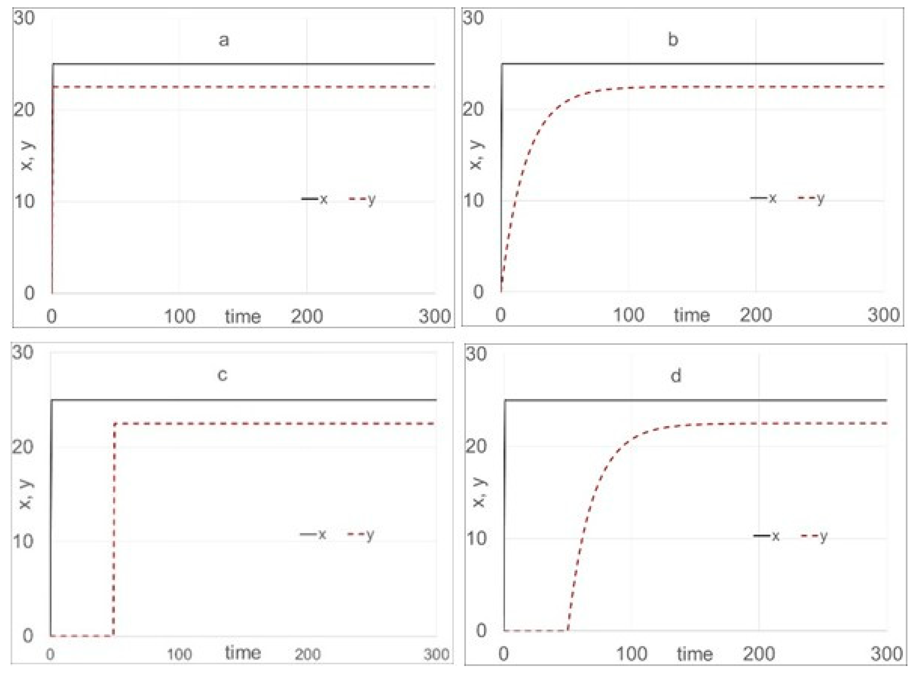
The response behavior of an output at time t, i.e., y_t, to changes in an input i at t, i.e., x_i,t, can be nondynamic (i.e., its total effect on y_t is immediate), or it can be dynamic (i.e., its total effect on y_t is not immediate). The two most common types of dynamic response behavior are dead-time (θ) and lag (τ). Figure 1 illustrates the nondynamic behavior and the effect these two types of dynamic behavior on y to a step change in the input, x, occurring at time t = 0. For the nondynamic response (a), y changes immediately to its new steady-state value. It is not correct to call this a steady-state case because steady state means “no change,” and in this example, x changes. Figure 1b illustrates lag since the change in y starts to occur at t = 0 and monotonically increases over time to its new steady-state value. Figure 1c illustrates dead-time since x changes at t = 0 but y does not change to its new value until some θ > 0 time later. Figure 1d illustrates lag and dead-time since x changes at t = 0 but y does not start to change until some θ > 0 time later and does not reach its new steady state immediately when it starts to change.

Examples of nondynamic changes include eyes opening (x) and immediate sight (y) and turning on the radio in a car (x) and hearing it (y) immediately. A dynamic time-delayed (i.e., dead-time) example is lightning occurring extremely far away. Lightning strikes first, followed by thunder, which is delayed and occurs significantly later. The sound does not gradually build up; instead, a sudden boom happens all at once. A dynamic lag occurs when a person has been in the cold for an extended period, causing their skin temperature to drop. Upon moving to a warmer environment, their skin temperature gradually rises, but it takes time to fully adjust to the new, warmer conditions.

When a system is dynamic, its mass and/or internal energy changes over time, being driven to a new state due to input changes, arriving there at a time different than when the input was changed. Mathematically (and theoretically), this is a time-order differential equation in y. Equation (2) below is a dynamic example with one input x and output y.

$$\begin{array}{l}{a}_n{\displaystyle \frac{d^{n}y(t)}{d{t}^n}}+a_{n-1}{\displaystyle \frac{d^{n-1}y(t)}{d{t}^{n-1}}}+\cdots +a_1{\displaystyle \frac{dy(t)}{dt}}+a_{0}y(t)=\\ \hspace{1em}{b}_m{\displaystyle \frac{d^{m}x(t-\theta )}{d{t}^m}}+b_{m-1}{\displaystyle \frac{d^{m-1}x(t-\theta )}{d{t}^{m-1}}}+\cdots +b_1{\displaystyle \frac{dx(t-\theta )}{dt}}+b_{0}x(t-\theta )\end{array}$$

(2)

2.2. Theoretically Based Dynamic Regression (TDR)

The proposed TDR approach uses backward difference derivatives (BDD) to discretize FOPDT and SOPDT theoretical dynamic systems [17,18,19]. The dynamic system does not have to be initially at a steady state for TDR modeling. Note that this initial condition is a common assumption in process dynamics and control textbooks [14,20], but this condition is not likely to be the case in real-world dynamic modeling and/or control applications [21].

Equations (3) and (4), below, are the theoretical (i.e., mathematical) representation for a one-input-one-output FOPDT system or process.

$$\tau {\displaystyle \frac{dv(t)}{dt}}+v(t)=x(t-\theta )$$

(3)

$$E[y(t)]=f(v(t))$$

(4)

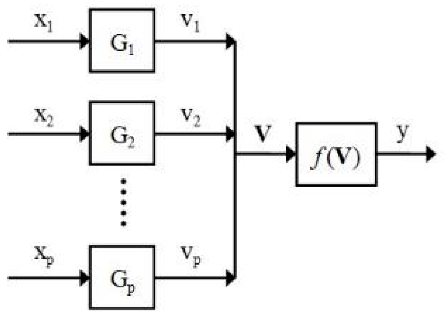
where $t\ge \theta ,$ x(t) is the value of the input variable at t, v(t) is the value of the output variable in the units of x at t, y(t) is the output variable in its units at t, and $E[y(t)]$ means the expected value of y(t), $f(v(t))$ is the true output (gain) function of v(t), such that $\tau \ge 0$ and $\theta \ge 0,$ for physical (i.e., theoretical) reasons. When $f(v(t))$ is a nonlinear function of v(t), Equations (3) and (4), taken together, have a Wiener block-oriented structure [17], as shown in Figure 2.

Backward difference discretization of Equation (3) gives:

$$\begin{array}{l}\widehat{\tau }\left({\displaystyle \frac{{\widehat{v}}_t-{\widehat{v}}_{t-\Delta t}}{\Delta t}}\right)+{\widehat{v}}_t=x_{t-(\widehat{\theta }+\Delta t)}\Rightarrow \left(\widehat{\tau }+\Delta t\right){\widehat{v}}_t=\widehat{\tau }{\widehat{v}}_{t-\Delta t}+\Delta t\hspace{0.17em}{x}_{t-(\widehat{\theta }+\Delta t)}\Rightarrow \\ {\widehat{v}}_t={\displaystyle \frac{\widehat{\tau }}{\widehat{\tau }+\Delta t}}{\widehat{v}}_{t-\Delta t}+{\displaystyle \frac{\Delta t}{\widehat{\tau }+\Delta t}}{x}_{t-(\widehat{\theta }+\Delta t)}=\widehat{\delta }{\widehat{v}}_{t-\Delta t}+\left(1-\widehat{\delta }\right)x_{t-(\widehat{\theta }+\Delta t)}\end{array}$$

(5)

where Δt is the constant sampling rate, and the “^” symbol means estimation because Equation (5) is a mathematical approximation of Equation (3) due to discretization, and as shown in Equation (5),

$$\widehat{\delta }={\displaystyle \frac{\widehat{\tau }}{\widehat{\tau }+\Delta t}}=1-{\displaystyle \frac{\Delta t}{\widehat{\tau }+\Delta t}}.$$

(6)

In Equation (5), $\widehat{\theta }$ is a positive integer of Δt, i.e., $\widehat{\theta }=m\Delta t,$ where m is a positive integer or 0. Note that, as shown in Equation (5), ${\widehat{v}}_t$ is nonlinear in $\widehat{\tau }$ and linear in $\widehat{\delta }$. We strongly recommend estimating τ and not δ to avoid ill conditioning, an artifact of linear regression but not of nonlinear regression. In addition, τ is physically interpretable, an advantage in physical understanding and for choosing starting values. Moreover, τ has physical constraints that protect against accepting estimates of parameters that fit well but are physically impossible (i.e., unrealizable). We illustrate the advantages of the use of τ over δ in the case below.

For practical implementation in modeling real data, we propose the following algorithm for FOPDT modeling:

$${\widehat{v}}_t=\left\{\begin{array}{l}{\displaystyle \frac{\widehat{\tau }}{\widehat{\tau }+\Delta t}}{\widehat{v}}_{t-\Delta t}+{\displaystyle \frac{\Delta t}{\widehat{\tau }+\Delta t}}{x}_{t-(\widehat{\theta }+\Delta t)},\hspace{1em}t>\widehat{\theta }=\widehat{m}\Delta t\\ {\widehat{v}}_{\widehat{\theta }}={\widehat{v}}_{\widehat{m}\Delta t}isestimated,\hspace{1em}t=\widehat{\theta }=\widehat{m}\Delta t\\ undefined,\hspace{1em}t<\widehat{\theta }=\widehat{m}\Delta t\\ Subjectto\widehat{\tau }>0,m\ge 0\end{array}\right.$$

(7)

Equation (7) is a physically (i.e., theoretically) constrained nonlinear regression estimation structure. In Equation (7), $\widehat{\tau }$ and $\widehat{\theta }$ (i.e., m) can be obtained using nonlinear regression along with input/output data. In addition, the initial value of $v_t,$ $v_{\widehat{\theta }}$, is also unknown. In the original development of this method, Ref. [17] proposed starting at process conditions where changes in y_t were minimal and setting ${\widehat{v}}_{\widehat{\theta }}$ to zero. In contrast, TDR treats $v_{\widehat{\theta }}$ as an unknown constant and estimates its value along with $\widehat{\tau }$ and $\widehat{\theta }$ using nonlinear regression. We found this approach to work well, as we will show. After obtaining ${\widehat{v}}_t,$ from Equation (7), the output, y_t, is estimated by Equation (8) below.

$${\widehat{y}}_t=\left\{\begin{array}{l}f({\widehat{v}}_t),\hspace{1em}t>\widehat{\theta }=\widehat{m}\Delta t\\ y_{\widehat{\theta }},\hspace{1em}t=\widehat{\theta }=\widehat{m}\Delta t\\ undefined,\hspace{1em}t<\widehat{\theta }=\widehat{m}\Delta t\end{array}\right.$$

(8)

A p-input version of Equation (3) is:

$${\tau }_i{\displaystyle \frac{d{v}_i(t)}{dt}}+v_i(t)=x_i(t-{\theta }_i),\hspace{1em}i=1,\dots ,p$$

(9)

y(t) = f(V(t))

(10)

where V(t) is a vector of v₁(t), …, v_p(t) and f(V(t)) is the mathematical function that maps V(t) to y(t). The multiple-input, backward difference, discrete-time version consists of changing ${\widehat{v}}_t,$ to ${\widehat{v}}_{i,t}$ and Equation (7) to its multiple-input form, as shown in Equation (11) below.

$${\widehat{v}}_{i,t}=\left\{\begin{array}{l}{\displaystyle \frac{{\widehat{\tau }}_i}{{\widehat{\tau }}_i+\Delta t}}{\widehat{v}}_{i,t-\Delta t}+{\displaystyle \frac{\Delta t}{{\widehat{\tau }}_i+\Delta t}}{x}_{i,t-({\widehat{\theta }}_i+\Delta t)},\hspace{1em}t>{\widehat{\theta }}_i={\widehat{m}}_i\Delta t\\ {\widehat{v}}_{{\widehat{\theta }}_i}={\widehat{v}}_{{\widehat{m}}_i\Delta t}isestimated,\hspace{1em}t={\widehat{\theta }}_i={\widehat{m}}_i\Delta t\\ undefined,\hspace{1em}t<{\widehat{\theta }}_i={\widehat{m}}_i\Delta t\\ Subjectto{\widehat{\tau }}_i>0,m_i\ge 0\end{array}\right.$$

(11)

A full second-order, discrete-time, linear regression function for f(V(t)) is:

$${\widehat{y}}_t=\left\{\begin{array}{l}f({\widehat{\mathrm{V}}}_t)={\widehat{a}}_0+{\widehat{a}}_1{\widehat{v}}_{1,t}+\cdots +{\widehat{a}}_p{\widehat{v}}_{p,t}+{\widehat{a}}_{11}{\widehat{v}}_{1,t}^2+\cdots +{\widehat{a}}_{pp}{\widehat{v}}_{p,t}^2\\ \hspace{1em}\hspace{1em}\hspace{0.17em}\hspace{0.17em}+{\widehat{a}}_{12}{\widehat{v}}_{1,t}{\widehat{v}}_{2,t}+\cdots +{\widehat{a}}_{p-1,p}{\widehat{v}}_{p-1,t}{\widehat{v}}_{p,t},\hspace{1em}\hspace{1em}\hspace{1em}\hspace{1em}\hspace{1em}\hspace{1em}\hspace{1em}t>{\theta }_{*}\\ {\widehat{a}}_0,\hspace{1em}\hspace{1em}\hspace{1em}\hspace{1em}\hspace{1em}\hspace{1em}\hspace{1em}\hspace{1em}\hspace{1em}\hspace{1em}\hspace{1em}\hspace{1em}\hspace{1em}\hspace{1em}\hspace{1em}\hspace{1em}\hspace{1em}\hspace{1em}\hspace{1em}\hspace{1em}t={\theta }_{*}\\ undefined,\hspace{1em}\hspace{1em}\hspace{1em}\hspace{1em}\hspace{1em}\hspace{1em}\hspace{1em}\hspace{1em}\hspace{1em}\hspace{1em}\hspace{1em}\hspace{1em}\hspace{1em}\hspace{1em}\hspace{1em}\hspace{1em}\hspace{1em}t<{\theta }_{*}\end{array}\right.\hspace{1em}$$

(12)

where ${\theta }_{*}={\widehat{\theta }}_{\max }$, i.e., the largest ${\widehat{\theta }}_i$ for a non-process control (i.e., a strictly dynamic modeling) application and ${\theta }_{*}={\widehat{\theta }}_{MV}$ (i.e., the estimated dead-time of the manipulated variable) for a process control application. Note that Equation (12) has the same structure as a static second-order linear regression function, with x replaced by v, and it contains no lag variables. Moreover, since the inputs are v_i’s and not x_i’s, Equation (12) is a TDR-class, multiple linear regression, and expectation function estimator.

Equation (13), below is a theoretical (i.e., mathematical) expression for a multiple-input, second-order-plus-dead-time-plus-lead (SOPDTPL), dynamic system or process [14].

$${\tau }_i^2{\displaystyle \frac{d^2{v}_i(t)}{d{t}^2}}+2{\tau }_i{\zeta }_i{\displaystyle \frac{d{v}_i(t)}{dt}}+v_i(t)={\tau }_{ai}{\displaystyle \frac{d{x}_i(t-{\theta }_i)}{dt}}+x_i(t-{\theta }_i)$$

(13)

The lead term is the first term on the right side of the equal sign. This term tends to “speed up” the response and provides what the process modeling and control community has termed “numerator dynamics”. For visual second-order behavior from one steady state to another steady state for particular domains of $\tau ,\zeta ,\mathrm{and} {\tau }_a$, see [14,17,20], which developed a second-order, multiple-input, single-output, discrete-time, nonlinear Wiener dynamic approach using backward difference derivatives (BDD) based on Equation (13). More specifically, using BDD approximation applied to a sampling interval of Δt, an approximate discrete-time form of Equation (13), for p inputs, is:

$${\widehat{v}}_{i,t}=\left\{\begin{array}{l}{\widehat{v}}_{i,t}={\widehat{\delta }}_{1,i}{\widehat{v}}_{i,t-\Delta t}+{\widehat{\delta }}_{2,i}{\widehat{v}}_{i,t-2\Delta t}+{\widehat{\omega }}_{1,i}{x}_{i,t-{\theta }_i-\Delta t}+{\widehat{\omega }}_{2,i}{x}_{i,t-{\theta }_i-2\Delta t},\hspace{1em}t>{\widehat{\theta }}_i={\widehat{m}}_i\Delta t\\ {\widehat{v}}_{{\widehat{\theta }}_i}={\widehat{v}}_{{\widehat{m}}_i\Delta t}isestimated,\hspace{1em}t={\widehat{\theta }}_i={\widehat{m}}_i\Delta t\\ undefined,\hspace{1em}t<{\widehat{\theta }}_i={\widehat{m}}_i\Delta t\\ Subjectto{\widehat{\tau }}_i>0,m_i\ge 0\end{array}\right.$$

(14)

where

$${\widehat{\delta }}_{1,i}={\displaystyle \frac{2{\widehat{\tau }}_i^2+2{\widehat{\tau }}_i{\widehat{\zeta }}_i\Delta t}{{\widehat{\tau }}_i^2+2{\widehat{\tau }}_i{\widehat{\zeta }}_i\Delta t+\Delta t^2}}$$

(15)

$${\widehat{\delta }}_{2,i}={\displaystyle \frac{-{\widehat{\tau }}_i^2}{{\widehat{\tau }}_i^2+2{\widehat{\tau }}_i{\widehat{\zeta }}_i\Delta t+\Delta t^2}}$$

(16)

$${\widehat{\omega }}_{1,i}={\displaystyle \frac{({\widehat{\tau }}_{ai}+\Delta t)\Delta t}{{\widehat{\tau }}_i^2+2{\widehat{\tau }}_i{\widehat{\zeta }}_i\Delta t+\Delta t^2}}$$

(17)

such that ${\widehat{\omega }}_{2,i}=1-{\widehat{\delta }}_{1,i}-{\widehat{\delta }}_{2,i}-{\widehat{\omega }}_{1,i}$ to satisfy the unity gain constraint and

$$G_{i,t}={\displaystyle \frac{v_{i,t}}{x_{i,\hspace{0.17em}t}}}={\displaystyle \frac{{\omega }_{i,1}B+\dots +{\omega }_{i,s}{B}^s}{1-{\delta }_{i,1}B-\dots -{\delta }_{i,r}{B}^r}}={\displaystyle \frac{{\omega }_i(B)}{{\delta }_i(B)}}$$

(18)

After obtaining ${\widehat{v}}_{i,t}$ for each input i, the modeled output value is determined by substituting these results into $f({\widehat{\mathrm{V}}}_t)$, such as the one given by Equation (12).

Process modeling and control textbooks, such as [14] and [20], have visual response examples of first- and second-order dynamic systems from their initial steady state to their new steady state for step input changes. When input changes are far enough apart, response plots can be sufficiently informative in choosing the model order and other behaviors. However, input changes are typically too frequent for visual examination to be helpful in identifying order and type of dynamic behavior. Our recommendation is to use the following model order strategy until the fit is sufficiently acceptable: 1. FO/FOPDT; 2. SO/SOPDT, $\zeta >1$; 3. SO/SOPDT, $0<\zeta \le 1$; 4. SO/SOPDT, $\zeta >1,{\tau }_a>0$; 6. SO/SOPDT, $\zeta >1,0<{\tau }_a$; 7. SO/SOPDT, $0<\zeta <1,{\tau }_a>0$; 8. SO/SOPDT, $0<\zeta <1,{\tau }_a<0$.

Model Identification and Summary Statistics

To avoid overfitting, we highly recommend using cross-validation as a supervised training approach that splits the data into two time-sequential sets—the training set $\left(t={\widehat{\theta }}_{\max },\dots ,t_{n_{tr}}\right)$ and the validation set $\left(t=t_{n_{tr}+1},\dots t_n\right)$, respectively [4]. We strongly recommend the use of the four (4) measures of performance given below to evaluate model fit. The first and most important is r_fit (which is bound between −1 and 1), the fitted correlation of the measured outputs, y_t, and the modeled outputs, ${\widehat{y}}_t,$ and is defined as:

$$r_{fit}=r_{y_t,{\widehat{y}}_t}={\displaystyle \frac{{\displaystyle \sum _{i=1}^n\left(y_i-\overline{y}\right)\left({\widehat{y}}_i-\overline{\widehat{y}}\right)}}{\sqrt{{\displaystyle \sum _{i=1}^n{\left(y_i-\overline{y}\right)}^2}}\cdot \sqrt{{\displaystyle \sum _{i=1}^n{\left({\widehat{y}}_i-\overline{\widehat{y}}\right)}^2}}}}$$

(19)

where n is the number of sampling times in the set. The TDR modeling objective is to find the largest possible positive value of r_fit in the validation set by changing the modeling parameters (i.e., all those with “^”) towards the minimum value of the sum of squared residuals (SSR) (often called the sum of squared errors, i.e., SSE) for the training data (SSRtr), as defined by Equation (20) below:

$$SSRtr={\displaystyle \sum _{i=m_{i,\max }}^{n_{tr}}{\left(y_i-{\widehat{y}}_i\right)}^2}$$

(20)

where m_i,max is the largest value of m_i, i.e., the one with the largest θ_i. The word “towards” is used here because the objective is not to find the values of the parameters that give the smallest value of SSRtr but the ones that give the largest value of r_fit for the validation set (i.e., r_fit,val). We note that using r_fit,val rather than SSR in the validation set (SSRval) is not common practice. However, since SSR is a measure of variability and not necessarily “fit,” we have found that using SSRval as an overfitting criterion can result in a substantial loss of fit. The drawback to using r_fit,val as opposed to SSRval is a greater tendency towards biased estimation. To address this drawback, we have obtained accurate results by first using SSRval and following this up (or finishing) with r_fit,val. Note that estimation bias can be addressed for the final trained model using the time series bias correction method described in [17].

The other two measures of performance that we recommend are for assessing, but not controlling, bias and closeness of fit. The third one, defined by Equation (21), is the average difference (AD):

$$AD={\displaystyle \frac{{\displaystyle \sum _{i=1}^n\left(y_i-\overline{y}\right)}}{n}}$$

(21)

AD is a measure of model bias, with zero as the smallest possible magnitude for this statistic. The final statistic, the average absolute difference (AAD), is defined as

$$AAD={\displaystyle \frac{{\displaystyle \sum _{i=1}^n\left|y_i-\overline{y}\right|}}{n}}$$

(22)

AAD is a measure of spread, i.e., variability. We prefer this measure over SSR because it is more easily interpretable, as roughly half of the values in a large data set will likely be greater than or less than its result since it is the mean absolute difference. To recap, our dynamic modeling goals are r_fit close to 1, with AD and AAD values being acceptably low.

It is important to understand that randomizing runs is not an option for modeling a dynamic system or process since data must be collected during dynamic transitions to obtain estimates of dynamic model coefficients. The nature of lag inherently controls the order of runs as systems change dynamically (see Figure 1). Furthermore, dynamic systems can only be modeled using dynamic data. Thus, the samples in a data set cannot be run in a random order, and time correlation/systematic bias is inherent. As a result, classical statistical inference, which requires full randomization runs, is not valid for dynamic modeling. Moreover, the four statistics above provide informal, not formal, measures of inference.

3. Results

This section consists of three real, freely existing data modeling cases to illustrate the strengths and effectiveness of TDR in modeling dynamic data. The first case, the weight model, illustrates the impact that one additional dynamic parameter can have on regression modeling. Thus, it illustrates the power of static modeling using v as the explanatory variable in place of x when the nature of the data is not static but dynamic. The second case compares the powerful empirical dynamic modeling method of Nonlinear Autoregressive Moving Average with eXogenous variables (NARMAX) [22,23,24,25,26,27,28] with TDR in eight test cases of a real pilot distillation column. The third case models SGC (y) using eleven explanatory variables (x_i). These data sets were modeled twice previously [18,19] for monitoring (i.e., without dead-time) but not for a forecast control application (with all inputs having a dead-time less than or equal to the insulin infusion dead-time of one hour), our current objective. This case illustrates the effectiveness of our current approach of forecast modeling for control for very large and stiff free-living data sets.

3.1. Weight Data Set Results

The second author provided a data set with the output (y) as the subject’s weight and several nutrient variables as the inputs. The data set covered a period of 9 years, during which time body weight was measured daily using a beam scale that was confirmed by a second measurement using a digital scale, and all food intake was weighed and recorded. The food intake was converted to individual nutrients by a nutritional database that includes information from the USDA Foods Database and many commercial sources, which was available through Calorie Count (sponsored by About.com) for the first 5.2 years and then through Nutritionix.com for the last 3.8 years of data collection. The data was compiled over consecutive 5-, 7-, or 10-day periods, with 28 occasional lapses of 5 to 28 days.

Given its limited size, our modeling work divided this data set into training and validation sets. Thus, our study does not include a test set. In addition, our objective is strictly modeling, rather than physiological assessments and interpretation. More specifically, our modeling objective is to obtain the highest r_fit,val to illustrate the modeling effectiveness of TDR in real, free-living modeling of highly dynamic data sets. Moreover, the modeling goal here is to achieve an r_fit,val > 0.90 for a relatively small set of input variables. The second author is interested in physiological understanding, and these results can provide a baseline fit for follow-up studies using other input combinations in this data set and other modeling ideas that she may have for this data set and other ones.

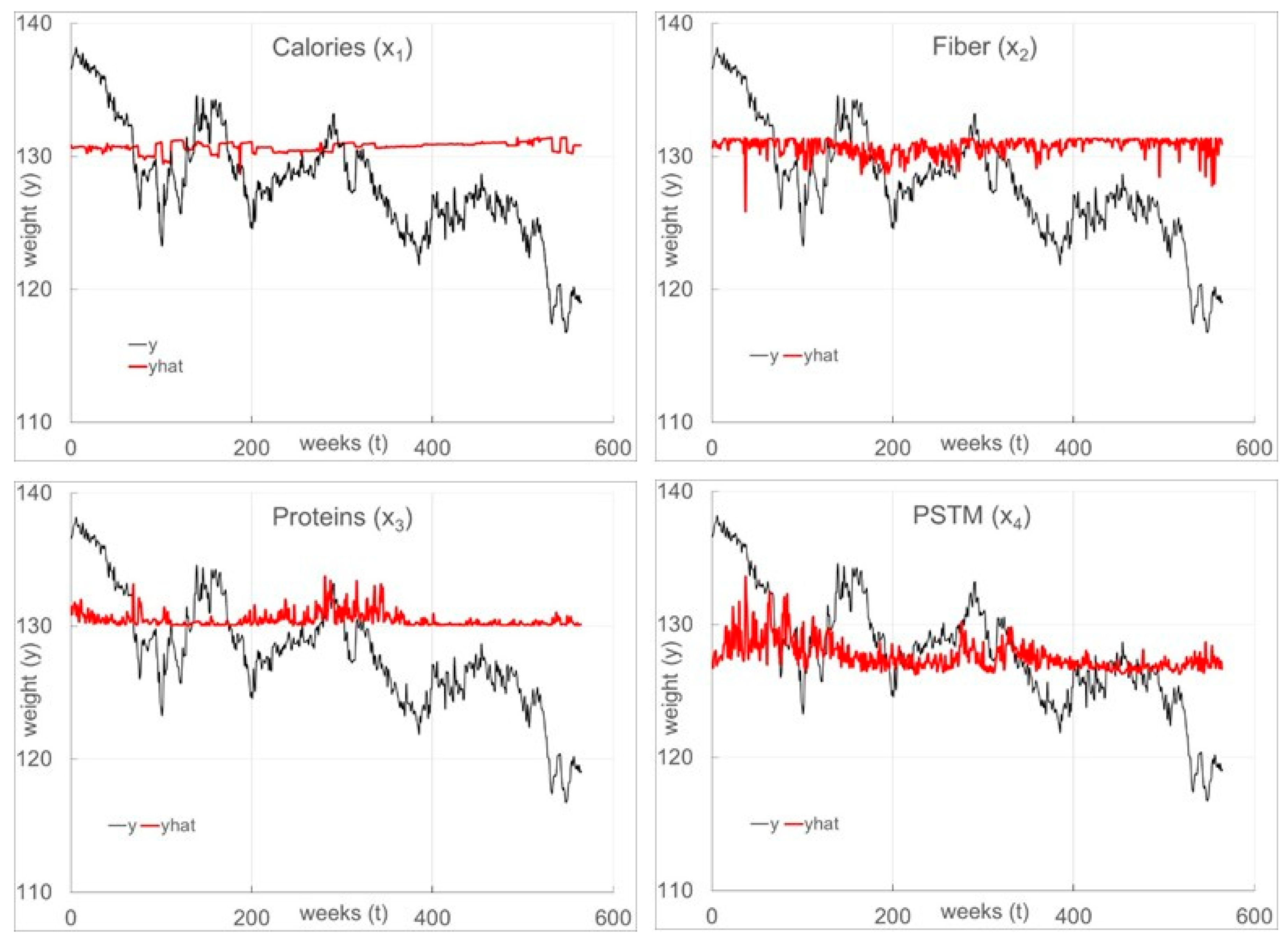
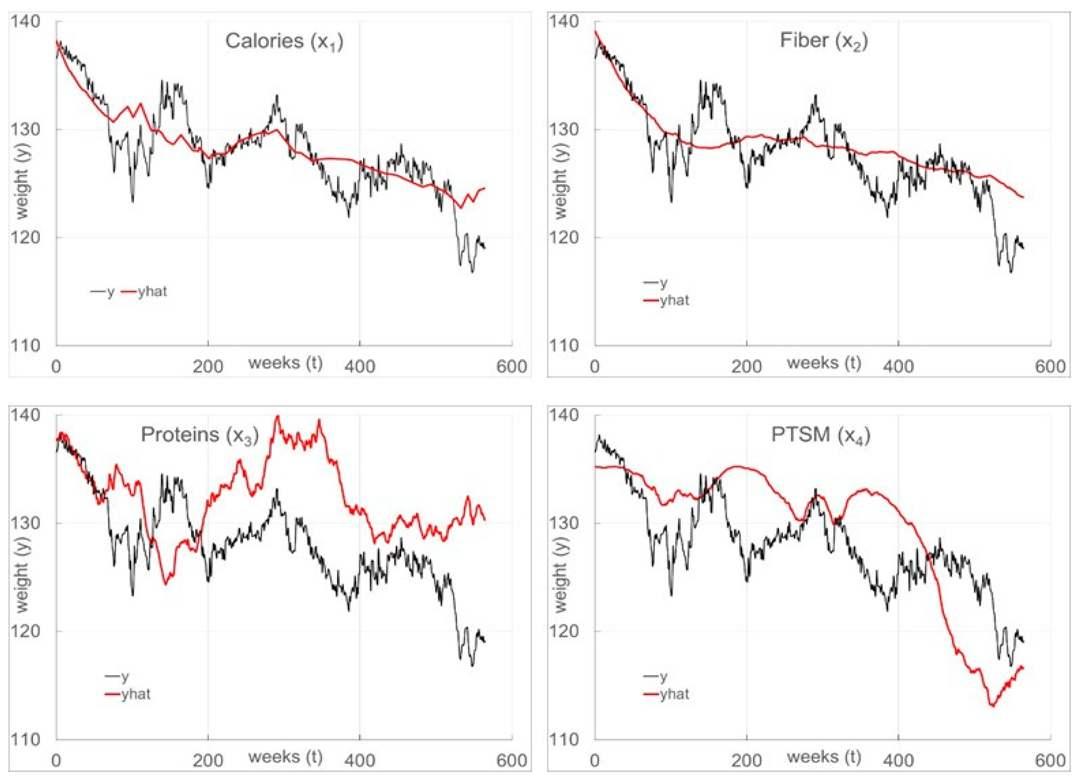
The full data set consisted of 14 nutrients: potassium, carbohydrates, calories, proteins, fats, sugar, saturated, cholesterol, fiber, vitamin A, vitamin C, calcium, iron, and salt. The sampling time, Δt, equals approximately one (1) week on average. The data covers a time range of 565Δt or about nine consecutive years. We found the following four inputs to best model the weight of this subject without any additional ones significantly impacting the fit: calories (x₁), fiber (x₂), proteins (x₃), and potassium (x₄). Single-input static (i.e., nondynamic) linear regression (SLR) and TDR results, with the same SLR structures, are given in

Table 1. Single-input SLR results for the weight modeling study.

i	rfit		AAD		AD		SSR
	Tr	Val	Tr	Val	Tr	Val	Tr	Val
1	0.11	−0.07	2.81	5.64	0.00	−5.52	3214.17	11,906.63
2	0.26	0.10	2.75	5.65	0.00	−5.52	3048.51	11,844.84
3	0.12	0.45	2.87	5.17	0.09	−5.10	3217.07	10,187.06
4	0.22	0.19	3.19	2.80	2.55	−1.80	5018.23	4065.84

and

Table 2. Single-input TDR results for the weight modeling study.

i	t (Weeks)	rfit		AAD		AD		SSR
		Tr	Val	Tr	Val	Tr	Val	Tr	Val
1	57.00	0.70	0.75	1.83	1.96	0.00	−0.75	1655.39	1763.23
2	82.15	0.73	0.75	1.69	2.28	0.04	−1.45	1519.67	2477.86
3	10.00	0.21	0.52	3.86	7.14	−1.71	−7.14	6029.05	17,776.75
4	100.00	0.41	0.58	3.45	5.19	2.55	−1.80	5200.98	10,156.87

, respectively, and graphical results are given in Figure 3 and Figure 4, respectively. The first half of these figures are the training model results, and the second half are the validation model results. TDR modeling for this data set is based on Equations (9) to (11), i.e., the first-order, multiple-input, dynamic modeling structure. Note that for protein, r_fit,val values are for a single-input static model, and the dynamic models are 0.450 and 0.517, respectively, indicating that protein appears to be only slightly dynamic.

As shown in

Table 3. Four-input SLR results for the weight modeling study.

Inputs		Calories (1)	Fiber (2)	Proteins (3)	Ptsm (4)
Linear	a0	a1	a2	a3	a4
	132.2996	−0.001	0.016	0.037	−0.001
Quadratic		a11	a22	a33	a44
		$-6.38\times {10}^{-7}$	0.0	$2.32\times {10}^{-6}$	$3.89\times {10}^{-7}$
Summary Statistics		rfit	AAD	AD	SSR
Training (n =282)		0.26	2.70	−0.0444	3040.11
Validation (n = 281)		0.30	5.56	−5.4921	11,533.45

(SLR) and

Table 4. Four-input TDR results for the weight modeling study.

Inputs		Calories (1)	Fiber (2)	Proteins (3)	Ptsm (4)
Linear	a0	a1	a2	a3	a4
	115.0001	0.084	−0.575	0.664	0.099
Quadratic		a11	a22	a33	a44
		$1.44\times {10}^{-6}$	$-6.57\times {10}^{-4}$	$1.21\times {10}^{-2}$	$-1.79\times {10}^{-4}$
i		1	2	3	4
ti		224.71	82.67	16.19	954.01
Summary Statistics		rfit	AAD	AD	SSR
Training (n =282)		0.92	1.03	−0.0035	521.63
Validation (n = 281)		0.91	1.96	−1.8486	1583.54

(TDR), with all four inputs in the model (the expectation functions are given in Equations (23) and (24), respectively), the structures consist of all eight (8) linear and quadratic terms. Note that v_i is determined from x_i based on Equation (11). As indicated in Table 4, the range for τ is 16 (protein) to 954 weeks. The plots showing the fits for both methods with all four inputs in the model are given in Figure 5. The TDR fit is excellent given the freely existing nature of this data set in contrast to the very poor SLR fit.

$${\mu }_{yt}=a_0+a_1{x}_{1,t}+a_2{x}_{2,t}+a_3{x}_{3,t}+a_4{x}_{4,t}+b_1{x}_{1,t}^2+b_2{x}_{,t2}^2+b_3{x}_{3,t}^2+b_4{x}_4^2$$

(23)

$${\mu }_{yt}=a_0+a_1{v}_{1,t}+a_2{v}_{2,t}+a_3{v}_{3,t}+a_4{v}_{4,t}+b_1{v}_{1,t}^2+b_2{v}_{2,t}^2+b_3{v}_{3,t}^2+b_4{v}_4^2$$

(24)

3.2. Distillation Data Sets Results

The weight case example in the previous section is static modeling versus dynamic modeling when the process is dynamic. This section compares dynamic methods, NARMAX versus TDR, using data generated by a real pilot distillation column obtained in [29]. NARMAX is a specific class of DR because of its empirical nature due to it using a lag variable. As a lag-based approach, NARMAX has all the limitations of DR in relation to TDR as mentioned above. In addition, since its structure is mathematically based and not physically based, obtaining good starting values can be significantly more challenging.

Ref. [30] randomly obtained ten (10) freely existing pilot distillation column data sets over a three-year period, including nine (9) inputs and one output. One data set was used for training, one for validation, and eight for testing. These data sets were generated by undergraduate chemical engineering students for their unit operation lab course. For the training data set, Ref. [30] could not find adequate starting values to obtain a NARMAX lagged-based fit for any of the ten data sets using MATLAB^® (Version 8.3). However, Ref. [29] derived the NARMAX BDD transfer functions given by Equation (25) below. Note that Equations (18) (Wiener) and (25) (NARMAX) differ only in their denominators. More specifically, Wiener BDD (Equation (18)) has a different denominator for each input, in contrast to NARMAX BDD (Equation (25)), which has the same denominator for each input. Using Equation (25), Ref. [29] successfully obtained training and validation NARMAX-BDD-fitted models for the distillation column data sets using Excel^®. Note that while Equations (18) and (25) look similar, Equation (18) is a theoretically based modeling structure and is derived from first-principle modeling (e.g., a dynamic component mass balance) and Equation (25) is an empirically based modeling structure and cannot be derived from first-principle modeling but from a structure (e.g., NARMAX) using lagged variables.

$$G_{i,t}={\displaystyle \frac{v_{i,t}}{x_{i,\hspace{0.17em}t}}}={\displaystyle \frac{{\omega }_{i,1}B+\dots +{\omega }_{i,s}{B}^s}{1-{\delta }_{1}B-\dots -{\delta }_r{B}^r}}={\displaystyle \frac{{\omega }_i(B)}{\delta (B)}}$$

(25)

After training/validating the model, the professor who oversees the lab arbitrarily (i.e., unbiasedly) obtained eight (8) test data sets over three years. The mean testing r_fit (i.e., r_fit,ts) values for Wiener TDR and NARMAX BDD were 0.84 and 0.28, respectively (see

Table 5. Wiener (WM) and NARMAX (NM) distillation model results.

Identification				WM			NM
Case	Date	Type	Duration (Min)	AD	AAD	rfit	AD	AAD	rfit
A	8 March 2008	Training	123	0.00	0.09	0.96	0.00	0.14	0.92
B	8 March 2008	Validating	122	−0.01	0.09	0.97	−0.22	0.24	0.92
C	22 March 2008	Testing	568	0.11	0.37	0.61	2.96	3.12	0.03
D	13 April 2008	Testing	391	0.17	0.24	0.82	2.62	2.62	0.20
E	5 June 2008	Testing	230	0.53	0.54	0.83	1.28	1.28	0.51
F	10 September 2008	Testing	142	0.54	0.54	0.93	3.51	3.51	0.39
G	24 September 2008	Testing	245	0.01	0.11	0.87	−0.03	0.20	0.85
H	22 May 2009	Testing	205	0.31	0.32	0.90	2.23	2.24	0.01
I	27 February 2011	Testing	130	−0.05	0.18	0.89	5.99	5.99	−0.03
J	24 March 2011	Testing	105	−0.14	0.19	0.90	0.69	0.81	0.30
Testing Absolute Mean				0.23	0.31	0.84	2.41	2.47	0.28
Testing Absolute StdDev				0.21	0.16	0.10	1.86	1.82	0.30

Notes: AD and AAD results are in degrees Celsius.

). Thus, in summary, for this distillation process, the TDR (WM) model was significantly better than the NARMAX BDD (NM) model, and NARMAX DR failed to model this process data.

3.3. Type 1 Diabetes Data Sets

Our third and final case presents the features and strengths of our TDR protocol for a forecast process control application. Our diabetes example serves this purpose and represents the first step in modeling this data set for a forecast control application. More specifically, the model structure for this case is a multiple-input, second-order, dynamic structure (see Equation (13)) with a first-order (i.e., linear) static structure. Thus, our objective is the completion of our first step, which is to obtain final or near-final estimates of the dynamic parameters using a first-order static function, the simplest one.

This third and final case consists of modeling SGC (y) for eleven (11) Type 1 diabetes data sets. Each one consists of about two weeks of free-living data, with a sensor glucose sampling rate of five (5) minutes. This context is feedback forecast control, where the controlled variable (CV) is SGC and the manipulated variable (MV) is exogenous (i.e., infused) insulin with a dead-time of θ_MV. Each data set has twelve inputs consisting of three (3) nutrients, seven (7) activity tracker variables, insulin infusion with bolus and basal injection amounts combined as one (1) input, and the time of day (i.e., a 24 h clock). The first author’s research group collected these data sets about 14 years ago when the Medtronic glucose sensor required replacement every three to four days and had a much longer warm-up period than current devices which are replaced weekly. Thus, the amount of missing SGC data is much higher than current Medtronic sensors. Subject-reported food logs for approximating carbohydrate, fat, and protein amounts are used. We note that while the activity tracker was innovative for this study at the time, it did not have the most critical sensor, in our opinion, heart rate. Moreover, its technology is considerably less advanced than today’s wearable activity devices and is thus obsolete by today’s standards. For more information about this study, see [18]. The eleven data sets are available publicly on the homepage of the first author.

Basically, forecasting is the use of current information to predict a future outcome. Weather forecasting seeks to predict future weather conditions but not change them. We call this “forecast monitoring” (FM). “Automatic forecast control” (AFC), our objective, seeks to accurately predict the future value of the controlled variable (CV) and then manipulate conditions in the present to drive the CV to its target (i.e., set point, SP) effectively after this future time distance is reached. Thus, AFC models must be “cause-and-effect” and developed and evaluated in outpatient studies. An FM methodology that models a correlation structure will fail in an outpatient, free-living, AFC study if it is not sufficiently “cause-and-effect”. All the SGC models that we have found in the literature model the correlation structure (e.g., see [30,31,32,33]).

Ref. [18] modeled these data sets using the second-order dynamic structure given by Equation (13) with the second-order, multiple linear regression, static structure given by Equation (12). They named this approach the Wiener Modeling Method (WMM). Ref. [17] extended WMM to a coupled modeling method (CMM) with the addition of unmeasured endogenous insulin. The WMM and CMM modeling results are very similar. However, as pointed out in [17], the critical benefits of CMM over WMM are the inference of the unmeasured endogenous insulin concentration and a sounder phenomenological understanding and behavior.

The first two data sets in this work (weight and distillation) have static response surfaces that are highly first-order (i.e., linear). However, for the diabetes data sets, the static response surfaces are highly nonlinear and highly interactive. These attributes make modeling these eleven data sets considerably more challenging.

The approach of [18], used for comparison with the proposed approach, had the following conditions and attributes in addition to the ones mentioned above. First, fifteen-minute meal announcements for all three food variables were used. Secondly, no dead-time was used for exogenous insulin or any inputs other than the three food variables. Thirdly, all modeling was carried out on one Excel^® worksheet. Fourthly, the following two-step model identification strategy was used to maximize validation, r_fit. In the first step, all the inputs and their dynamic parameters were fitted simultaneously using a first-order static model. Its best fit served as the starting point for the second step, i.e., to find the best full (i.e., second-order) model fit (see Equation (12)).

The following two procedures were the same for [18] and the proposed TDR approach for feedback control. Firstly, missing activity data were estimated by averaging the two values on both sides of a gap and filling in the gap with this value. Some gaps were several hours long. Secondly, cross-validation was used, with the first week as the training (Tr) data set and the second week as the validation (Val) data set, to guard against overfitting the models.

As our knowledge has evolved, we have come to recognize critical and unique challenges in modeling SGC that this proposed forecast modeling TDR (f-TDR) approach overcomes. The first, and perhaps most critical, is the dead-time application. An accurate method to estimate the dead-time for exogenous insulin (θ_MV) and the appreciation of the criticality of θ_MV as the modeled dead-time for all inputs, except those with announcements, was not known or understood by the original modelers. Insulin injection decreases blood glucose concentration (BGC) but not until an unknown time after injection. For these eleven subjects, insulin injections are highly correlated with increasing and high SGC because these subjects tended to inject insulin when their BGC was high or from the knowledge that it would be increasing. However, any model with θ_MV too small (as in the WMM and CMM studies) will have a physiologically incorrect increase in SGC behavior with increasing insulin infusion (i.e., a positive correlation). It is critical to note that the WMM and CMM models had dead-time (i.e., θ > 0) for only the food variables, as mentioned above. Thus, this modeling condition alone makes the WMM and CMM approaches unacceptable for a control modeling application such as this one. It is critical to note that, in this context, θ_MV is not actually the exogenous insulin dead-time but what we call “the model effective dead-time,” which is the value that has the detectably correct phenomenological behavior and gives the best fit of the model to the data. Next, we explain how we estimate θ_MV.

The proposed f-TDR approach has the correct exogenous insulin (i.e., MV) cause-and-effect relationship for process control and significantly improves soundness, admissibility, and r_fit, in comparison to the WMM and CMM studies, using the following novel modeling protocol. Firstly, combining bolus and basal insulin reduced the number of inputs by one. Secondly, with only the insulin input in the model, and starting with θ_MV equal to 60 min, we moved θ_MV one sample distance (i.e., 5 min) at a time in the direction of increasing r_fit,val until r_fit,val stopped increasing. Using this scheme, we estimated the model effective dead-time, θ_MV $\left(\mathrm{i}.\mathrm{e}., {\widehat{\theta }}_{MV}\right),$ to be 60 min (12Δt), or close to this value, in all 11 modeling cases. Thirdly, for each input i, we used an f-TDR dead-time rule of ${\widehat{\theta }}_i \ge {\widehat{\theta }}_{MV},$ except for the announcement inputs and time of day (since its value is known for any time in the future). This criterion is necessary because real-time model prediction is a forecasting application since an MV change does not detectably affect SGC until θ_MV time in the future. Fourthly, for each input, f-TDR obtains an SOPDTPL (i.e., Equation (13)) dynamic and first-order static fit (i.e., Equation (12) with one input) on its own (i.e., individual) Excel^® worksheet. This simplest static structure is used because the focus is on obtaining good starting values for the dynamic parameters one input at a time and for each input separately.

As this process proceeds, the single-input fitted results are examined and evaluated based on fitting unique dynamic information in the data. To maximize this objective, we applied a strategy of using different starting values. Fifthly, each input’s fitted first-order static parameter and dynamic parameters are transferred to one Excel^® worksheet as starting values for fitting the multiple-input model.

For each subject, starting with carbohydrates, then insulin, then the two other food inputs, then the tracker inputs, and, lastly, time of day, a multiple-input, second-order dynamic (i.e., Equation (13) for each input) and a first-order static (i.e., Equation (12) with α_ij = 0, $\forall i,j$) fitted structure is obtained in two steps. The first step, one input at a time, varies its dynamic parameters, the static intercept, and its first-order static parameter to improve the validation fit for the f-TDR multiple-input static model. The input is retained in the model if, and only if, r_fit,val improves. The second step seeks to further improve r_fit,val by allowing all retained static parameters to change with all the dynamic parameters fixed.

Ref. [18] modeling results using the (WMM) full model static, multiple-input structure and our first-order static, multiple-input f-TDR structure are given in

Table 6. WMM ¹ and f-TDR ² SG model results.

Subject		WMM		f-TDR
		θ = 0		θ = 60 min
		Tr	Val	Tr	Val
1	501	0.61	0.68	0.67	0.77
2	502	0.49	0.51	0.73	0.75
3	503	0.68	0.66	0.62	0.67
4	504	0.53	0.55	0.52	0.61
5	505	0.56	0.55	0.73	0.59
6	506	0.67	0.68	0.67	0.75
7	507	0.69	0.64	0.59	0.65
8	508	0.45	0.43	0.35	0.62
9	509	0.63	0.56	0.64	0.60
10	510	0.57	0.73	0.50	0.72
11	511	0.72	0.79	0.76	0.74
Mean		0.60	0.62	0.62	0.68
Minimum		0.45	0.43	0.35	0.59
Maximum		0.72	0.79	0.76	0.77

¹ WMM results are inadmissible full-order static results for this f-TDR process control application. ² f-TDR results are first-order admissible static results for this process control application.

. Keep in mind, as explained above, that the WMM approach of [18] is not admissible in this forecast control application. As Table 6 shows, WMM, even with its full static and ${\widehat{\theta }}_i =0$ versus ${\widehat{\theta }}_i \ge {\widehat{\theta }}_{MV}$ modeling advantages, the mean f-TDR r_fit,val is significantly higher, more specifically, 0.68 versus 0.62. In addition, the smallest f-TDR r_fit,val is 0.59 versus 0.43 for WMM.

For one f-TDR case, Subject 11, we fit a static linear regression model structure with significant second-order interactions and third-order main effects. It resulted in an r_fit,val of 0.79, significantly better than 0.74 but not substantially better. In addition, we performed it one term at a time to keep from overextending the optimization tool, and thus, the modeling exercise required substantial time, expertise, and effort. Stepwise linear regression algorithms [34] cannot be used in this application because, to our knowledge, none exist for cross-validation. However, since artificial neural network (ANN) algorithms are designed for nonlinear static modeling and inherently use cross-validation, our future work to improve the fit of these eleven (11) data sets will focus on new ways to apply ANN algorithms and tools to extend this f-TDR approach to nonlinear dynamic and nonlinear static Wiener BDD modeling structures using a cross-validation tool-box. This work will use a new and novel physically informed dynamic nonlinear modeling approach [35,36].

4. Discussion

4.1. Weight Data Set

As indicated in Table 1, only one SLR r_fit,val result is above 0.2. It is for x₃ and is 0.45. However, its r_fit training (i.e., r_fit,tr) value is only 0.12. Moreover, the visual fits in Figure 3 show that essentially no significant SLR fits the data for training or validation. In contrast, as shown in Table 2 for TDR, r_fit,val ranges from 0.52 to 0.75 with two training values above 0.70, one respectable at 0.41, and one low at 0.21. Figure 4 shows the single-input TDR graphical results. In contrast to the SLR results in Figure 3, the TDR models follow the decreasing and increasing trends in the data over time substantially better than the SLR models.

As shown in Table 3, all the four-input SLR results are quite poor in comparison to the TDR results. Mainly, note that SLR r_fit,tr is 0.26 and r_fit,val is 0.30. In contrast, as shown in Table 4, the TDR-modeled four-input results are excellent and much better than those obtained with SLR. More specifically, r_fit,tr and r_fit,val are 0.92 and 0.91, respectively. The fitted plots in Figure 5 show the poor fitting of SLR in comparison to TDR for the four-input case. This contrast in fit between SLR and TDR is the result of one additional parameter, τ, for each input. These values are given in Table 4 and range from 16.2 weeks to 954.0 weeks.

Thus, with the addition of one parameter for each input, the TDR model substantially improved the fit of the response for this data set. DR may have been able to achieve this as well but would have required several additional parameters because the lag behavior of this data set is extensive (it has a τ = 954 weeks for one of the inputs!) and, thus, would cause DR modeling to be substantially more complex. In addition, the lag coefficients would not be physically interpretable with the defined constraints, as mentioned above.

The following is an example fitting a one-input (for simplicity of illustration), first-order dynamic (see Equation (7)) and second-order (i.e., quadratic) static TDR model. The purpose of this exercise is to aid readers in understanding how to build and fit TDR models. The starting guessed value of v₀, v_0guess, is 5. Example results for t = 3 and t = 4 are given in

Table 7. Data table for this example.

t	$\widehat{\mathit{v}}$	x	y	$\widehat{\mathit{y}}$	${\mathit{e}}_{\mathit{t}}$	${\mathit{e}}_{\mathit{t}}^2$
3	5.00	10	31	23.5	7.5	56.3
4	6.67	12	33	36.6	−3.6	13.0
$⋮$	$⋮$	$⋮$	$⋮$	$⋮$	$⋮$	$⋮$

. Other conditions and values are as follows:

$$\begin{array}{l}\theta =\hspace{0.17em}3,\hspace{1em}{\widehat{v}}_0={\widehat{v}}_1={\widehat{v}}_2={\widehat{v}}_3=5.00,\hspace{1em}{x}_0=x_1=x_2=x_3=10,\hspace{0.17em}\hspace{1em}{x}_t=12\hspace{0.17em}for\hspace{0.17em}t\ge 4,\\ {\widehat{v}}_t={\displaystyle \frac{\widehat{\tau }}{\widehat{\tau }+\Delta t}}{\widehat{v}}_{t-\Delta t}+{\displaystyle \frac{\Delta t}{\widehat{\tau }+\Delta t}}{x}_{t-(\widehat{\theta }+\Delta t)};\hspace{1em}{\widehat{v}}_4={\displaystyle \frac{\widehat{\tau }}{\widehat{\tau }+\Delta t}}{\widehat{v}}_3+{\displaystyle \frac{\Delta t}{\widehat{\tau }+\Delta t}}{x}_0,\hspace{1em} \\ \hspace{0.17em}\hspace{0.17em}{\widehat{\tau }}_{guess}=\hspace{0.17em}\widehat{\tau }\hspace{0.17em}=\hspace{0.17em}2,\hspace{0.17em}\Delta t=1,\hspace{0.17em}\hspace{1em}{\widehat{v}}_4={\displaystyle \frac{2}{2+1}}5.00+{\displaystyle \frac{1}{2+1}}10=20/3=6.67,\hspace{0.17em}\hspace{0.17em}\\ {\widehat{y}}_t={\widehat{\beta }}_0+{\widehat{\beta }}_1{\widehat{v}}_t+{\widehat{\beta }}_{11}{\widehat{v}}_t^2,\hspace{0.17em}{\widehat{y}}_3=1+2(5)+0.5\left(5^2\right)=23.5,\hspace{0.17em}{\widehat{y}}_4=1+2(6.67)+0.5\left({6.67}^2\right)=36.6\\ y_3=31,\hspace{0.17em}{y}_4=33,\hspace{0.17em}{e}_t=y_t-{\widehat{y}}_t,\hspace{1em}{e}_3=31-23.5=7.5,\hspace{1em}{e}_4=33-36.6=-3.6\end{array}$$

4.2. Distillation Data Sets

As presented in the previous section, the Wiener BDD (mean testing r_fit = 0.84) approach significantly fit the eight (8) distillation testing data sets better than NARMAX BDD (mean testing r_fit = 0.28). NARMAX DR in MATLAB^® failed to fit in all cases. The pairwise correlation matrices provide insight into these r_fit results.

With all the inputs having the same denominator in Equation (25) for NARMAX BDD, the expectation is that its V sample correlation matrix would have more significantly correlated pairs than its X correlation matrix and pairs with much higher correlation. This expectation is supported by the correlation matrices in [29] and reproduced in

Table 8. Training set correlation matrix for the input variables.

	x1	x2	x3	x4	x5	x6	x7	x8	x9
x1	1.00	0.01	0.14	0.22	−0.14	0.13	−0.03	0.15	−0.11
x2		1.00	0.65	0.01	−0.09	0.04	0.02	0.36	−0.18
x3			1.00	0.01	0.07	0.08	0.01	0.56	−0.12
x4				1.00	−0.16	0.93	0.91	0.11	0.13
x5					1.00	−0.10	−0.06	0.10	0.16
x6						1.00	0.88	0.11	0.13
x7							1.00	0.10	0.05
x8								1.00	−0.04
x9									1.00

,

Table 9. Training set correlation matrix for NARMAX BDD.

	v1	v2	v3	v4	v5	v6	v7	v8	v9
v1	1.00	0.52	0.59	0.21	0.51	−0.07	−0.02	0.72	0.41
v2		1.00	0.80	0.12	0.30	0.02	−0.02	0.85	0.70
v3			1.00	0.16	0.44	0.05	−0.03	0.79	0.70
v4				1.00	0.20	0.81	0.85	0.22	0.09
v5					1.00	−0.04	−0.02	0.60	0.38
v6						1.00	0.78	0.03	0.08
v7							1.00	−0.01	−0.02
v8								1.00	0.81
v9									1.00

and

Table 10. Training set correlation matrix for Wiener TDR.

	v1	v2	v3	v4	v5	v6	v7	v8	v9
v1	1.00	0.08	0.09	0.24	0.15	0.11	−0.03	0.08	0.36
v2		1.00	0.79	−0.02	−0.02	0.03	0.04	0.47	−0.08
v3			1.00	0.02	0.22	0.03	0.02	0.63	−0.12
v4				1.00	0.14	−0.86	−0.73	0.23	0.07
v5					1.00	0.04	−0.01	0.27	0.35
v6						1.00	0.80	−0.21	0.04
v7							1.00	−0.33	0.00
v8								1.00	−0.05
v9									1.00

given below. Results with absolute values of 0.5 or greater are in bold and red text. In contrast, Wiener BDD did not have more or much higher pairwise correlations, and some were even significantly lower in V than in X. Thus, the Wiener BDD method is supported to have an increasing cause-and-effect impact, and NARMAX BDD seems to have a decreasing one, in comparison.

5. Conclusions

As illustrated above, the proposed Theoretically based Dynamic Regression (TDR) methodology has several strengths/advantages over lagged-based methods (LBMs) such as Dynamic Regression (DR) and Nonlinear Autoregressive Moving Average with eXogenous variables (NARMAX), as demonstrated in this manuscript. The first one is TDR’s use of theoretically based dynamic model structures, as they can capture dynamic behavior in as little as one parameter, e.g., τ, as illustrated in the human weight data case in Section 4. In contrast, LBMs, due to their empirical nature, can require many lag parameters to adequately model even the simplest, i.e., first-order, dynamic behavior, and thus, this is a less parsimonious approach than TDR. Their limitations also include parameters without physical interpretation (unlike τ, the residence time), complexities of obtaining initial values to facilitate convergence, and no control over obtaining physically unrealizable (i.e., impossible) estimates. In addition, as LBM parametrization increases, model complexity increases, which decreases the likelihood of successful optimal model identification. This LBM drawback is illustrated in Section 4 for the distillation column process in the NARMAX modeling failure using MATLAB^®.

In addition to the principle of parsimony being a critical strength of TDR over LBMs, to effectively apply TDR, one does not have to have extensive knowledge in theoretical dynamic modeling because even very complex high-order dynamic systems can often be sufficiently modeled by first-order or second-order dynamic structures, i.e., by Equation (9) or (13), respectively (see [14]). Thus, the learning curve for statisticians and others not trained in first-principle dynamic modeling is simply the contents of this manuscript, i.e., Equations (9) and (13). Another critical strength of TDR is the full use of static (i.e., classic) regression methodologies and structures because of the one-to-one replacement of x_t with v_t (e.g., see Equation (12)), as illustrated in all the examples in this work. This is not the case with LBMs since its transformation of inputs can require several lagged variables of x_t and y_t (e.g., see Equation (1)), and thus, this is a critical drawback due to its inability to exploit classical regression structures and methodologies. Very critically, the human weight data case illustrates how static regression can fail tremendously when it is applied to a dynamic system.

The TDR model structure has two basic parts—a dynamic part and a static part. The dynamic part is based on first-principle dynamic modeling with theoretically based structures (what has been called “grey box modeling”), physically interpretable parameters, and physically defined constraints. Thus, its role is to transform the static inputs, i.e., x_i’s, into their theoretically interpretable dynamic counterparts, i.e., the v_i’s (see Figure 2). To achieve this objective, TDR uses backward difference derivatives (BDD) of theoretical first-order (Equation (9)) or second-order (Equation (13)) differential equations. Thus, the advantages of TDR over DR (including NARMAX) include fewer parameters, using parameters with phenomenological meaning, including physical interpretation and physical constraints, and exploiting classical static regression modeling and methodologies (i.e., non-lagged variable static structures). More specifically, physically based dynamic modeling structures, such as those given by Equations (9) and (13), transform the static x_i’s into the dynamic v_i’s and f(X) becomes f(V).

In this work, all modeling cases consist of real, freely existing data, i.e., data not generated by fixed or experimentally designed input changes from modeler influence. As mentioned in this section above, the classical NARMAX LBM approach failed to fit a model to the distillation data using MATLAB^®. Applying the BDD approach to NARMAX yielded a set of transfer functions for each input with the same denominator, a structure that causes greater pairwise correlation in the elements of V and, thus, it adversely affected model performance as well as cause-and-effect modeling compared to the BDD physically interpretable (i.e., first-principle) transformation developed in [17]. Thus, even with the advantage of the BDD transformation, NARMAX has critical limitations compared to TDR.

The weight data set is an example of modeling for understanding. Thus, its goal is a high r_fit with a small set of predictors. Four (4) of fourteen possible predictors produced static linear regression models with training and validation r_fit values of 0.26 and 0.30, respectively, and TDR values of 0.92 and 0.91, respectively. Thus, given this remarkable TDR model achievement with this type of data, these results could help lead to a better understanding and ideas for future directions for nutritional scientists.

The weight data example has a simple first-order dynamic and simple static (i.e., quadratic) structure. The distillation example has a more complex second-order dynamic and a simple first-order static structure. The modeling for these two examples is complete. The diabetes data sets have highly complex static and dynamic structures. The modeling in this work focused on modeling the dynamic structure, and thus, the static structure was first-order. Future modeling of the diabetes data sets will focus on developing non-linear static techniques to significantly improve model fit. One idea is a two-stage approach where the dynamic structures and results of this work are fixed, and a non-linear regression structure and approach is used, such as an ANN. Another approach will model the nonlinear static and second-order dynamic parameters simultaneously in a one stage approach. We have completed cases of both approaches, and the results are very promising.

TDR success is highly dependent on the data set having the necessary inputs, sampling rate, and running time to adequately cover the desired input space and obtain sufficient sizes of training, validation, and test data. Moreover, at the core of the TDR approach is the idea that many dynamic systems or processes can be adequately approximated by FOPDT or SOPDT structures. However, when this is not the case, dynamic structures that adequately represent the dynamic behavior (e.g., third-order) will have to be used. In addition, there could be true dynamic structures that do not approximate sufficiently accurately, or an application requires high accuracy that can only be obtained via theoretical modeling or highly accurate semi-theoretical modeling. When modeling requires dynamic and spatial structures, more sophisticated versions of TDR will need to be developed and applied.

References

1. Pefia, D. Measuring Influence in Dynamic Regression Models. Technometrics 1991, 33, 93–101. [Google Scholar] [CrossRef]
2. Maekawa, K.; Yamamoto, T.; Takeuchi, Y.; Hatanaka, M. Estimation in Dynamic Regression with an Integrated Process. J. Stat. Plan. Inference 1996, 49, 279–303. [Google Scholar] [CrossRef]
3. Pollock, D.S.G.; Pitta, E. The Misspecification of Dynamic Regression Models. J. Stat. Plan. Inference 1996, 49, 223–239. [Google Scholar] [CrossRef]
4. Diniz, C.A.R.; Rodrigues, C.P. The Lag Length of a Dynamic Regression Model: A Comparative Study. AIP Conf. Proc. 2008, 1073, 150–156. [Google Scholar] [CrossRef]
5. Costa, L.; Smith, J.Q.; Nichols, T. A Group Analysis Using the Multiregression Dynamic Models for fMRI Networked Time Series. J. Stat. Plan. Inference 2019, 198, 43–61. [Google Scholar] [CrossRef]
6. Akaike, H. A New Look at the Statistical Model Identification. IEEE Trans. Autom. Control 1974, 19, 716–723. [Google Scholar] [CrossRef]
7. Schwarz, G. Estimating the Dimension of a Model. Ann. Stat. 1978, 6, 461–464. [Google Scholar] [CrossRef]
8. Villani, M. Fractional Bayesian Lag Length Inference in Multivariate Autoregressive Processes. J. Time Ser. Anal. 2001, 22, 67–86. [Google Scholar] [CrossRef]
9. Li, M.; Gençay, R. Tests for Serial Correlation of Unknown Form in Dynamic Least Squares Regression with Wavelets. Econ. Lett. 2017, 155, 104–110. [Google Scholar] [CrossRef]
10. Huang, Y. Restoration of Monotonicity Respecting in Dynamic Regression. J. Am. Stat. Assoc. 2017, 112, 613–622. [Google Scholar] [CrossRef]
11. Haugh, L.D.; Box, G.E.P. Identification of Dynamic Regression (Distributed Lag) Models Connecting Two Time Series. J. Am. Stat. Assoc. 1977, 72, 121–130. [Google Scholar] [CrossRef]
12. Martinussen, T.; Scheike, T.H. Dynamic Regression Models for Survival Data; Springer Science & Business Media: Berlin/Heidelberg, Germany, 2007; ISBN 978-0-387-33960-3. [Google Scholar]
13. Duncan, D.B.; Horn, S.D. Linear Dynamic Recursive Estimation from the Viewpoint of Regression Analysis. J. Am. Stat. Assoc. 1972, 67, 815–821. [Google Scholar] [CrossRef]
14. Seborg, D.E.; Edgar, T.F.; Mellichamp, D.A. Process Dynamics and Control, 2nd ed.; Wiley: Hoboken, NJ, USA, 2003; ISBN 978-0-471-00077-8. [Google Scholar]
15. Neshasteriz, A.R.; Khaki Sedigh, A.; Sadjadian, H. Generalized Predictive Control and Tuning of Industrial Processes with Second Order plus Dead Time Models. J. Process Control 2010, 20, 63–72. [Google Scholar] [CrossRef]
16. Alfaro, V.M.; Vilanova, R. Model-Reference Robust Tuning of 2DoF PI Controllers for First- and Second-Order plus Dead-Time Controlled Processes. J. Process Control 2012, 22, 359–374. [Google Scholar] [CrossRef]
17. Rollins, D.K.; Bhandari, N.; Kleinedler, J.; Kotz, K.; Strohbehn, A.; Boland, L.; Murphy, M.; Andre, D.; Vyas, N.; Welk, G.; et al. Free-Living Inferential Modeling of Blood Glucose Level Using Only Noninvasive Inputs. J. Process Control 2010, 20, 95–107. [Google Scholar] [CrossRef]
18. Kotz, K.; Cinar, A.; Mei, Y.; Roggendorf, A.; Littlejohn, E.; Quinn, L.; Rollins, D.K., Sr. Multiple-Input Subject-Specific Modeling of Plasma Glucose Concentration for Feedforward Control. Ind. Eng. Chem. Res. 2014, 53, 18216–18225. [Google Scholar] [CrossRef] [PubMed]
19. Rollins, D.; Goeddel, C.E.; Matthews, S.L.; Mei, Y.; Roggendorf, A.; Littlejohn, E.; Quinn, L.; Cinar, A. An Extended Static and Dynamic Feedback–Feedforward Control Algorithm for Insulin Delivery in the Control of Blood Glucose Level. Ind. Eng. Chem. Res. 2015, 54, 6734–6748. [Google Scholar] [CrossRef]
20. Smith, C.A.; Corripio, A.B. Principles and Practices of Automatic Process Control, 3rd ed.; Wiley: Hoboken, NJ, USA, 2005; ISBN 978-0-471-43190-9. [Google Scholar]
21. Sinha, D. Dynamic Regression Models for Survival Data. J. Am. Stat. Assoc. 2007, 102, 1474. [Google Scholar] [CrossRef]
22. Nelles, O. Nonlinear System Identification; Springer: Berlin/Heidelberg, Germany, 2001; Volume 13. [Google Scholar]
23. Hambali, N.; Rahiman, M.H.F.; Taib, M.N.; Yassin, A.I.M. A Review on Nonlinear Modeling for Steam Distillation System and Its Significance. In Proceedings of the 2016 IEEE 12th International Colloquium on Signal Processing & Its Applications (CSPA), Melaka, Malaysia, 4 March–6 March 2016; ISBN 978-1-4673-8780-4. [Google Scholar]
24. Shariff, H.M.; Marzaki, M.H.; Rahiman, M.H.F. A Study of Nonlinearity Behavior in System Dynamic for Steam Distillation Essential Oil Extraction System. In Proceedings of the 2014 IEEE 5th Control and System Graduate Research Colloquium, Shah Alam, Malaysia, 11–12 August 2014; pp. 176–180. [Google Scholar] [CrossRef]
25. El Mghouchi, Y.; Udristioiu, M.T.; Yildizhan, H.; Brancus, M. Forecasting Ground-Level Ozone and Fine Particulate Matter Concentrations at Craiova City Using a Meta-Hybrid Deep Learning Model. Urban Clim. 2024, 57, 102099. [Google Scholar] [CrossRef]
26. Lin, M.; Chi, R.; Sheng, N. Data Driven Latent Variable Adaptive Control for Nonlinear Multivariable Processes. Int. J. Syst. Sci. 2024, 56, 108–125. [Google Scholar] [CrossRef]
27. Stefanoiu, D.; Culita, J.; Voinea, A.-C.; Voinea, V. Nonlinear Identification for Control by Using NARMAX Models. Mathematics 2024, 12, 2252. [Google Scholar] [CrossRef]
28. Bernat, J.; Kołota, J.; Superczyńska, P. NARMAX Approach for the Identification of a Dielectric Electroactive Polymer Actuator. Int. J. Control Autom. Syst. 2023, 21, 3080–3090. [Google Scholar] [CrossRef]
29. Rollins, D.; Roggendorf, A.; Khor, Y.; Mei, Y.; Lee, P.; Loveland, S. Dynamic Modeling With Correlated Inputs: Theory, Method, and Experimental Demonstration. Ind. Eng. Chem. Res. 2015, 54, 2136–2144. [Google Scholar] [CrossRef]
30. Stahl, F.; Johansson, R. Short-Term Diabetes Blood Glucose Prediction Based on Blood Glucose Measurements. In Proceedings of the 2008 30th Annual International Conference of the IEEE Engineering in Medicine and Biology Society, Vancouver, BC, Canada, 20–25 August 2008; pp. 291–294. [Google Scholar]
31. Georga, E.I.; Protopappas, V.C.; Polyzos, D. Prediction of Glucose Concentration in Type 1 Diabetic Patients Using Support Vector Regression. In Proceedings of the 10th IEEE International Conference on Information Technology and Applications in Biomedicine, Corfu, Greece, 3–5 November 2010; pp. 1–4. [Google Scholar]
32. Allam, F.; Nossair, Z.; Gomma, H.; Ibrahim, I.; Abd-el Salam, M. Prediction of Subcutaneous Glucose Concentration for Type-1 Diabetic Patients Using a Feed Forward Neural Network. In Proceedings of the 2011 International Conference on Computer Engineering & Systems, Kuantan, Malaysia, 27–29 July 2011; pp. 129–133. [Google Scholar]
33. Levine, M.E.; Hripcsak, G.; Mamykina, L.; Stuart, A.; Albers, D.J. Offline and Online Data Assimilation for Real-Time Blood Glucose Forecasting in Type 2 Diabetes. arXiv 2017, arXiv:1709.00163. [Google Scholar] [CrossRef]
34. Devore, J. Probability and Statistics for Engineering and the Sciences, 9th ed.; Cengage Learning: Boston, MA, USA, 2015; ISBN 978-1-305-25180-9. [Google Scholar]
35. Pun, G.P.P.; Batra, R.; Ramprasad, R.; Mishin, Y. Physically Informed Artificial Neural Networks for Atomistic Modeling of Materials. Nat. Commun. 2019, 10, 2339. [Google Scholar] [CrossRef] [PubMed]
36. Isaev, A.; Dobroserdova, T.; Danilov, A.; Simakov, S. Physically Informed Deep Learning Technique for Estimating Blood Flow Parameters in Four-Vessel Junction after the Fontan Procedure. Computation 2024, 12, 41. [Google Scholar] [CrossRef]
Figure 1. Response of y, a first-order (FO) dynamic system in (b) b and (d), to a step change in input x: (a) nondynamic; (b) lag; (c) dead-time; (d) lag and dead-time.
Stats 08 00089 g001
Figure 2. Block diagram for the Wiener network with p inputs and one output. Each input, xi, is passed through its own unity gain linear dynamic block, Gi, after which these unobservable intermediate outputs are collected and passed through a single unrestricted static gain function, f(V), to produce the output, y.
Stats 08 00089 g002
Figure 3. The SLR measured (y) and fitted ( y ^ ) weight for x1 to x4.
Stats 08 00089 g003
Figure 4. The single-input TDR measured (y) and fitted ( y ^ ) weight plots for x1 to x4.
Stats 08 00089 g004
Figure 5. The multiple-input (x1 to x4) TDR (left) and SLR (right) measured (y) and fitted ( y ^ ) plots.
Stats 08 00089 g005