A Simulation-Based Comparative Analysis of Two-Parameter Robust Ridge M-Estimators for Linear Regression Models

Abstract

Traditional regression estimators like Ordinary Least Squares (OLS) and classical ridge regression often fail under multicollinearity and outlier contamination respectively. Although recently developed two-parameter ridge regression (TPRR) estimators improve efficiency by introducing dual shrinkage parameters, they remain sensitive to extreme observations. This study develops a new class of Two-Parameter Robust Ridge M-Estimators (TPRRM) that integrate dual shrinkage with robust M-estimation to simultaneously address multicollinearity and outliers. A Monte Carlo simulation study, conducted under varying sample sizes, predictor dimensions, correlation levels, and contamination structures, compares the proposed estimators with OLS, ridge, and the most recent TPRR estimators. The results demonstrate that TPRRM consistently achieves the lowest Mean Squared Error (MSE), particularly in heavy-tailed and outlier-prone scenarios. Application to the Tobacco and Gasoline Consumption datasets further validates the superiority of the proposed methods in real-world conditions. The findings confirm that the proposed TPRRM fills a critical methodological gap by offering estimators that are not only efficient under multicollinearity, but also robust against departures from normality.

1. Introduction

Linear regression (LR) is a foundational statistical technique that models the relationship between a dependent variable and one or more independent variables. It can range from simple linear regression, which uses a single predictor, to multiple linear regression (MLR) that incorporates numerous predictors, thus allowing for a more comprehensive understanding of how various factors influence the dependent variable. The mathematical form of MLRM [1] is

$$y=X\beta +\epsilon$$

(1)

where y denotes an n × 1 vector of response variables, and X represents a known n × p matrix of predictor variables. The vector β is a p × 1 vector of unknown regression parameters, while ε is an n × 1 vector of error terms, satisfying E(ε) = 0 and V(ε) = σ² I_n, where I_n is the n × n identity matrix. Typically, the Ordinary Least Squares (OLS) method is used to estimate the model parameters; it is a widely adopted approach due to its efficiency and ease of interpretation [2]. OLS estimation calculates the regression coefficients by minimizing the sum of squared residuals, thereby fitting the best linear line to the data. The simplicity of this method has made it a cornerstone in statistical analysis, but it requires various assumptions to ensure the validity and reliability of its predictions. The OLS of β is defined as

$$\begin{array}{l}{\hat{\beta }}_{OLS}=V^{-1}X\prime y\end{array}$$

(2)

where V = $X\prime X$. OLS is the best linear unbiased estimator under some classical assumptions, like no correlation among predictors, i.e., no multicollinearity, no outliers, finite error variance, and correct model specification. Studies have shown that the above OLS estimator can yield inaccurate results when these model assumptions are violated [3]. However, even in the presence of multicollinearity, the OLS estimator retains optimal prediction properties under the classical assumptions of no outliers and finite error variance. However, in finite samples or when variance inflation becomes severe, the OLS estimates may become unstable, leading to poor practical performance [4]. In such cases, ridge regression [5] introduces a small bias that reduces variance, yielding more stable coefficient estimates and, in practice, improved predictive performance, particularly in finite samples or in data prone to noise and outliers. This adjustment helps to improve the model’s accuracy and prevents the coefficient estimates from becoming excessively large in the presence of highly correlated predictors. Ridge regression is therefore valuable in refining the predictive capacity of MLR models, especially when multicollinearity is unavoidable due to the nature of the data. From 1970 until now, almost 400 estimators have been suggested in the literature to combat the problem of MC [6]. The ridge regression estimator of β is defined as

$${\hat{\beta }}_k={(\mathrm{V}+kI)}^{-1}X\prime y,$$

(3)

where k > 0 is the ridge or shrinkage parameter. To enhance the efficiency of the ridge estimator, ref. [7] introduced an additional parameter, termed ‘q’, alongside k, resulting in the two-parameter ridge regression (TPRR) estimator, which is defined as

$${\hat{\beta }}_{q,k}= \stackrel{̑}{q}(X\prime X+kI{)}^{-1}X\prime y,$$

(4)

where

$$\stackrel{̑}{q}={\displaystyle \frac{\left(X\prime y\right)\prime (X\prime X+kI{)}^{-1}X\prime y}{\left(X\prime y\right)\prime (X\prime X+kI{)}^{-1}X\prime X(X\prime X+kI{)}^{-1}X\prime y}}$$

(5)

The value of ‘q’ in the above equation is derived by maximizing the coefficient of determination, while the value of ‘k’ is chosen to minimize the Mean Squared Error (MSE). It is important to note that k and q are shrinkage parameters, whereas the ridge regression and its two-parameter extensions are the corresponding estimators that utilize these parameters. This distinction is crucial, as the efficiency of an estimator depends on how appropriately its shrinkage parameters are chosen.

Notable work in the area of two-parameter estimators has been conducted in [8,9,10,11,12]. To simultaneously address multicollinearity and outliers, robust ridge M-estimators were introduced in [13] based on the work of [14,15]. The objective function for the robust M ridge regression used in [13] was based on Huber’s loss function [16].

$$\stackrel{⌢}{\beta }=\arg {\min }_{\beta }\left[{\displaystyle \sum _{i=1}^n\rho \left(\frac{y_i-x_i^T\beta }{\delta }\right)+\lambda {‖\beta ‖}^2}\right]$$

(6)

These M-based ridge regression estimators demonstrate a smaller Mean Squared Error (MSE) compared to traditional ridge regression estimators. Recent advancements in this area have been made in [17,18,19]. The same concept of using M estimators to derive a robust version of a ridge estimator was extended to the two-parameter ridge regression approach by Ertaş et al. in 2015, by combining the benefits of robust M-estimation and the most efficient two-parameter ridge regression in order to handle both MC and outliers effectively [20]. Recent work in this area was conducted in [21].

Now, motivated by the idea of Ertas et al., the purpose of this study is to refine existing techniques and develop more adaptive and resilient estimation frameworks. This study proposes and evaluates a new TPRRM approach to tackle the combined challenges of MC and outliers. Through simulation studies and numerical examples, the research aims to demonstrate that these new estimators outperform existing methods. The goal of this paper is to improve the reliability and accuracy of regression models in datasets that are rich in outliers, contributing to more informed and effective decision-making in statistical modeling.

The organization of the paper is as follows: Section 2 presents the methodology, along with an introduction to the proposed estimator. A simulation study is conducted in Section 3. Section 4 illustrates the advantages of the proposed estimator using the Tobacco and Gasoline Consumption datasets. Some concluding remarks are presented in Section 5.

2. Materials and Method

For mathematical convenience, regression is expressed in canonical form. Equation (1), in orthogonal form, is

$$y=P\alpha +\epsilon$$

(7)

Here, $P=XD$, and $\alpha =C\prime \beta$, C is an orthogonal matrix containing eigen vectors of X′X such that $C\prime C=I_p$ and $\Lambda =C\prime \mathrm{X}\prime \mathrm{X}\mathrm{C}$ = $\Lambda =diag({\lambda }_1,{\lambda }_2,{\lambda }_3,\dots ,{\lambda }_p)$, where ${\lambda }_i$ are the ordered eigen values of matrix X′X. $I_p$ is the identity matrix of order p. Now the canonical form of Equations (2) and (3) is

$${\stackrel{⌢}{\alpha }}_{OLS}={\Lambda }^{-1}\mathrm{P}\prime y$$

(8)

$${\stackrel{⌢}{\alpha }}_k={(\Lambda +k{I}_p)}^{-1}\Lambda {\stackrel{⌢}{\alpha }}_{OLS}$$

(9)

The canonical form of the M estimator of the above equation is

$${\stackrel{⌢}{\alpha }}_{k,M}={(\Lambda +k{I}_p)}^{-1}\Lambda {\stackrel{⌢}{\alpha }}_M$$

(10)

The canonical form of Equation (4) is

$${\stackrel{⌢}{\alpha }}_{k,TP}=q{(\Lambda +k{I}_p)}^{-1}\Lambda {\stackrel{⌢}{\alpha }}_{OLS}$$

(11)

The canonical form of the M estimator of the above equation is

$${\stackrel{⌢}{\alpha }}_{k,TP,M}=q{(\Lambda +k{I}_p)}^{-1}\Lambda {\stackrel{⌢}{\alpha }}_M$$

(12)

Here, ${\stackrel{⌢}{\alpha }}_M$ is an M estimator such that $\stackrel{⌢}{\alpha }=C\prime \stackrel{⌢}{\beta }$ and $MSE(\stackrel{⌢}{\alpha })=MSE(\stackrel{⌢}{\beta })$. The canonical forms of the OLS, ridge, robust ridge, and two-parameter ridge estimators are presented in Equations (8)–(12). The Mean Squared Errors (MSEs) of these estimators are given in (13)–(18), with robust versions based on [22].

$$MSE({\stackrel{⌢}{\alpha }}_{OLS})={\displaystyle \sum _{i=1}^p\left(\frac{{\stackrel{⌢}{\sigma }}^2}{{\lambda }_i}\right)}$$

(13)

$$MSE({\stackrel{⌢}{\alpha }}_M)={\displaystyle \sum _{i=1}^p\left(\frac{{\hat{A}}^2}{{\lambda }_i}\right)}={\displaystyle \sum _{i=1}^p{\Omega }_{ii}}$$

(14)

$$MSE({\stackrel{⌢}{\alpha }}_k)={\displaystyle \sum _{i=1}^p\left(\frac{{\lambda }_i{\stackrel{⌢}{\sigma }}^2}{{({\lambda }_i+k)}^2}\right)}+{\displaystyle \sum _{i=1}^p\left(\frac{k^2{\stackrel{⌢}{\alpha }}_{OLS}^2}{{({\lambda }_i+k)}^2}\right)}$$

(15)

$$MSE({\stackrel{⌢}{\alpha }}_{k,M})={\displaystyle \sum _{i=1}^p\left(\frac{{\lambda }_i{\hat{A}}^2}{{\lambda }_i{({\lambda }_i+k)}^2}\right)}+{\displaystyle \sum _{i=1}^p\left(\frac{k^2{\stackrel{⌢}{\alpha }}_M^2}{{({\lambda }_i+k)}^2}\right)}$$

(16)

$$MSE({\stackrel{⌢}{\alpha }}_{k,TP})=q^2{\displaystyle \sum _{i=1}^p\left(\frac{{\lambda }_i{\stackrel{⌢}{\sigma }}^2}{{({\lambda }_i+k)}^2}\right)}+{{\displaystyle \sum _{i=1}^p\left(\frac{q{\lambda }_i}{{\lambda }_i+k}-1\right)}}^2{\stackrel{⌢}{\alpha }}_{OLS}^2$$

(17)

$$MSE({\stackrel{⌢}{\alpha }}_{k,TP,M})=q^2{\displaystyle \sum _{i=1}^p\left(\frac{{\lambda }_i{\hat{A}}^2}{{({\lambda }_i+k)}^2}\right)}+{{\displaystyle \sum _{i=1}^p\left(\frac{q{\lambda }_i}{{\lambda }_i+k}-1\right)}}^2{\stackrel{⌢}{\alpha }}_M^2$$

(18)

Here, ${\stackrel{⌢}{A}}^2={\displaystyle \frac{s^2\left[{\left(n-p\right)}^{-1}{\displaystyle \sum _{i=1}^p{\psi }^2\left({\in }_i/s\right)}\right]}{{\left[n^{-1}{\displaystyle \sum _{i=1}^p\psi \prime \left({\in }_i/s\right)}\right]}^2}}$, ${\stackrel{⌢}{\delta }}^2$ is replaced by $A^2$, where $A^2$ is a robust estimator based on the M-estimator proposed by [23].

2.1. Existing Estimators

• The groundbreaking ridge estimator introduced by Hoerl & Kennard (1970a) is as follows [5]:

  $${\hat{k}}_{H{K}_1}={\displaystyle \frac{{\hat{\sigma }}^2}{{\hat{\alpha }}_i^2}} where,i=1,2,3,\dots ,p$$

  (19)

  where ${\hat{\sigma }}^2={\displaystyle \frac{{\left(y-X\hat{\beta }\right)}^T\left(y-X\hat{\beta }\right)}{n-p-1}}.$
• The second ridge estimator introduced by Hoerl & Kennard (1970b) is as follows [24]:

$${\hat{k}}_{H{K}_2}={\displaystyle \frac{{\stackrel{⌢}{\sigma }}^2}{{\stackrel{⌢}{\alpha }}_{\max }^2}}$$

(20)

3.

Ref. [14] generalized the idea of Hoerl & Kennard (1970a) and suggested a new estimator, denoted as HKB:

$${\hat{k}}_{HKB}={\displaystyle \frac{p{\stackrel{⌢}{\sigma }}^2}{{\displaystyle \sum _{i=1}^p{\stackrel{⌢}{\alpha }}_i^2}}}$$

(21)

4.

Kibria (2003) suggested three new ridge regression estimators by taking the AM, GM, and Median of Hoerl & Kennard (1970a, ref. [5]) [25]:

$${\hat{k}}_{AM}={\displaystyle \frac{1}{p}}{\displaystyle \sum _{i=1}^p\frac{{\stackrel{⌢}{\sigma }}^2}{{\stackrel{⌢}{\alpha }}_i^2}}$$

(22)

$${\hat{k}}_{GM}={\displaystyle \frac{{\stackrel{⌢}{\sigma }}^2}{{\left({\displaystyle \prod _{i=1}^p{\stackrel{⌢}{\alpha }}_i^2}\right)}^{\frac{1}{p}}}}$$

(23)

$${\hat{k}}_{MED}=Med\left({\displaystyle \frac{{\stackrel{⌢}{\sigma }}^2}{{\stackrel{⌢}{\alpha }}_i^2}}\right)$$

(24)

5.

Similarly, Khalaf et al. (2013) proposed an estimator by combining the idea of Hoerl & Kennard (1970b, ref. [24]) with the concept of weight, as follows [26]:

$${\hat{k}}_{KMS}=\left({\displaystyle \frac{{\lambda }_{\max }}{{\displaystyle \sum _{i=1}^p{\stackrel{⌢}{\alpha }}_i^2}}}\right)\left({\displaystyle \frac{{\stackrel{⌢}{\sigma }}^2}{{\stackrel{⌢}{\alpha }}_{\max }^2}}\right)$$

(25)

These estimators reduce instability in coefficient estimates caused by multicollinearity, yet they remain sensitive to outliers. Their performance deteriorates under contamination, which limits their applicability in real-world data, where assumptions of normality and clean samples rarely hold.

2.2. Two-Parameter Ridge Regression Estimator

• To improve the fit quality of the one-parameter ridge regression, ref. [7] recommended using the k value defined in Equation (20) along with the parameter ‘q’ from Equation (5), thus introducing the concept of the two-parameter robust ridge regression estimator (TPRRE) [7].
• Inspired by [7], Toker & Kaçiranlar (2013) introduced a new TPRRE based on optimal selection of the k and q values [8].

$${\stackrel{⌢}{q}}_{opt}={\displaystyle \frac{{\displaystyle \sum _{i=1}^p\frac{{\stackrel{⌢}{\alpha }}_i^2{\lambda }_i}{{\lambda }_i+k}}}{{\displaystyle \sum _{i=1}^p\frac{{\stackrel{⌢}{\sigma }}^2{\lambda }_{i+}{\stackrel{⌢}{\alpha }}_i^2{\lambda }_i}{{({\lambda }_i+k)}^2}}}}$$

(26)

$${\stackrel{⌢}{k}}_{opt}={\displaystyle \frac{{\hat{q}}_{opt}{\displaystyle \sum _{i=1}^p{\stackrel{⌢}{\sigma }}^2{\lambda }_i+({\hat{q}}_{opt}-1){\displaystyle \sum _{i=1}^p{\stackrel{⌢}{\alpha }}_i^2{\lambda }_i}}}{{\displaystyle \sum _{i=1}^p{\stackrel{⌢}{\alpha }}_i^2{\lambda }_i}}}$$

(27)

3.

The latest advancements in the field of TPRRE were introduced by Khan et al. (2024) [11], who proposed six new estimators with the goal of enhancing the accuracy of ridge estimation.

$${\hat{k}}_{SH1}={\displaystyle \frac{{\lambda }_{\max }-100{\lambda }_{\min }}{99}}$$

(28)

$${\hat{k}}_{SH2}={\lambda }_{\max }-100{\lambda }_{\min }$$

(29)

$${\hat{k}}_{SH3}={\lambda }_{\max }-{\lambda }_{\min }$$

(30)

$${\hat{k}}_{SH4}={\displaystyle \frac{{\lambda }_{\max }}{{\lambda }_{\min }}}$$

(31)

$${\hat{k}}_{SH5}={\lambda }_{\max }$$

(32)

$${\hat{k}}_{SH6}={\lambda }_{min}$$

(33)

Recent contributions by [11] propose six new TPRR estimators, further improving estimation under MC. However, their framework does not account for robustness against non-normal errors and outliers. As such, while TPRR improves efficiency through two shrinkage parameters, it still inherits the vulnerability of ridge-type estimators to contaminated data.

2.3. Proposed Estimator

Now, motivated by the idea of [12,20,21], we propose Two-Parameter Robust Ridge M-Estimators (TPRRM). The novelty lies in embedding dual shrinkage parameters within a robust M-estimation framework, thereby achieving efficiency under multicollinearity while ensuring resilience to outliers. Unlike existing two-parameter estimators, the proposed TPRRM preserves the strengths of dual shrinkage while mitigating contamination effects. Through both simulation and application to the Tobacco dataset, we empirically demonstrate that TPRRM consistently outperforms classical ridge, robust ridge, and the most recent TPRR estimators.

The proposed estimators are as follows.

Ref. [26] suggested a weight for ridge estimators as follows:

$$w_{KMS}={\displaystyle \frac{{\lambda }_{\max }}{{\displaystyle \sum _{i=1}^p{\stackrel{⌢}{\alpha }}_i^2}}}$$

(34)

Following [19], we modified Equation (34) and used its M-version, as follows:

$$w_m={\displaystyle \frac{{\lambda }_{\max }}{\frac{{\displaystyle \sum _{i=1}^p{\stackrel{⌢}{\alpha }}_{iM}}}{p}}}$$

(35)

We multiplied Equations (28)–(33) by Equation (35) and obtained our six new proposed estimators, BAD1, BAD2, BAD3, BAD4, BAD5, and BAD6, which are given below:

$${\hat{k}}_{BAD1}=\left({\displaystyle \frac{{\lambda }_{\max }-100{\lambda }_{\min }}{99}}\right)*w_m$$

(36)

$${\hat{k}}_{BAD2}=\left({\lambda }_{\max }-100{\lambda }_{\min }\right)*w_m$$

(37)

$${\hat{k}}_{BAD3}=({\lambda }_{\max }-{\lambda }_{\min })*w_m$$

(38)

$${\hat{k}}_{BAD4}=\left({\displaystyle \frac{{\lambda }_{\max }}{{\lambda }_{\min }}}\right)*w_m$$

(39)

$${\hat{k}}_{BAD5}=({\lambda }_{\max })*w_m$$

(40)

$${\hat{k}}_{BAD6}=({\lambda }_{min})*w_m$$

(41)

The above value of k will be used in Equation (5) to calculate the value of $\hat{q}$. Then both $\hat{q}$ and $\hat{k}$ value will be put into Equation (4) to estimate $\stackrel{⌢}{\beta }.$

A simulation study is performed in the section below to compare the performance of the suggested estimator with that of existing estimators.

3. Simulation Study

3.1. Simulation Design

To examine the performance of the proposed and existing estimators under diverse conditions, a Monte Carlo simulation experiment incorporating varying levels of multicollinearity, error variance, sample sizes, and numbers of predictors has been used. The data-generating process was adapted from the work of [11,18,27,28].

The predictor variables were generated as follows:

$$x_{ij}=\left(\sqrt{1-{\rho }^2}{z}_{ji}+\rho z_{jp+1}\right), for \left(i=1,2,3,\dots , p\right) and \left(j=1,2,3,\dots ,n\right)$$

(42)

where z_ij ∼ N(0,1) and ρ denotes the correlation between regressors. This design ensures that the predictors exhibit the desired degree of multicollinearity.

To capture a wide range of conditions, we consider pairwise correlations as ρ = {0.85, 0.90, 0.95, 0.99, 0.999}, ranging from moderate to near-perfect multicollinearity. The number of predictors is p = {4, 10} and the sample size is n = {20, 50, 100}.

The regression coefficients β were generated using the Most Favorable (MF) direction approach, which ensures comparability across estimators [12]. Without loss of generality, the intercept term was set to zero. The error term ε_i was generated from two distributions: normal distribution, ε_i ∼ N(0,σ²), and heavy-tailed distribution, εi ∼ Cauchy (0,1). The variance parameter was varied across four levels, σ² = {0.5, 1, 5, 10}, allowing us to assess estimator performance under both low- and high-noise conditions.

To assess robustness, contamination was introduced by replacing randomly selected response values (y_j) with values shifted in the y-direction. Two contamination levels were considered, 10% and 20%, generated by taking the error variance as ‘σ² + 10’ and ‘σ² + 20’ respectively. For robust ridge M-type estimators, the Huber objective function is used in conjunction with the ‘rlm()’ function to calculate the M-estimator.

The response variable was then computed as follows:

$$y_j={\alpha }_0+{\alpha }_1{x}_{ij}+{\alpha }_2{x}_{2j}+\dots +{\alpha }_p{x}_{pj}+{\epsilon }_j, for i = 1, 2, 3,\dots , p and j = 1, 2, 3,\dots ,n$$

(43)

3.2. Performance Evaluation Criteria

Unlike OLS, ridge estimators introduce a certain degree of bias. The MSE criterion provides a more appropriate basis for evaluating and comparing such biased estimators, as mentioned by [10,12]. Furthermore, the existing literature consistently emphasizes the use of the minimum MSE criterion as the standard for identifying the most efficient estimator [12,19,27]. The MSE is defined as

$$MSE(\stackrel{⌢}{\alpha })=E\left[\left(\stackrel{⌢}{\alpha }-\alpha \right)\prime \left(\stackrel{⌢}{\alpha }-\alpha \right)\right]$$

(44)

Each scenario was replicated 5000 times to ensure stable results. The estimated MSE (EMSE) was computed as follows:

$$MSE(\stackrel{⌢}{\alpha })={\displaystyle \frac{1}{5000}}{\displaystyle \sum _{j=1}^{5000}\left({\stackrel{⌢}{\alpha }}_j-\alpha \right)\prime \left({\stackrel{⌢}{\alpha }}_j-\alpha \right)}$$

(45)

All simulations and calculation were performed using R version 4.5.1 programing language, and the results are summarized in both tabular and graphical form.

3.3. Simulation Results Discussion

Table 1, Table 2, Table 3 and Table 4 (and Supplementary Tables S1–S8) illustrate the estimated Mean Squared Error (MSE) of estimators for normally distributed errors with 10% and 20% outliers in the response variable. Table 5 contains comprehensive data for the Cauchy distribution. Table 6 provides a bird’s-eye view of all the situations considered in the simulation study of the proposed and existing estimators, and thoroughly reviews the top-performing estimators for all situations studied. Figure 1 is the diagnostic plot confirms the presence of three outliers (green dots), which are clearly separated from the fitted model (red dots and line), supporting the use of a BAD4. This plot visually demonstrates how the estimator is not influenced by these extreme data points, thereby producing a more reliable regression fit.

Table 1. Estimated MSE values with $n=25$, $p=4$, and 10% outliers in the y-direction.

${\mathit{\sigma }}^2=0.1$					${\mathit{\sigma }}^2=1$
$\mathit{\rho }$	0.85	0.95	0.99	0.999	0.85	0.95	0.99	0.999
OLS	6.54715199	20.95106882	105.5304231	1066.107042	8.78480056	27.33002393	139.1731178	1345.611102
HK	3.33311058	10.47577522	52.14910175	525.7322212	4.51098404	13.83365763	70.61252185	669.4597999
HKB	1.94987753	5.57549348	26.39481325	263.6889613	2.59025794	7.31764713	36.07807873	334.5928801
KAM	0.51929794	0.39756238	0.24831816	0.21161024	0.7286564	0.77529207	0.86278377	0.44779355
KMS	1.42824372	7.761373	69.62319025	972.668171	2.19101398	11.39166435	97.70809437	1239.587147
LC	4.00838268	12.25215963	60.2990279	605.6202206	5.51814168	16.45496312	82.64997568	783.1625333
ST	36,880.4599	11,807.55971	319.6213161	38.78512917	19,398.96541	17,193.6689	336.9727693	190.8436776
SH1	14.81471775	14.05215153	8.92650916	1.3568562	18.52235209	18.64904267	12.75262638	1.85909349
SH2	0.08559237	0.19857319	0.07770096	0.07376037	0.11696336	0.29742759	0.11235643	0.09623571
SH3	0.19472094	0.09973364	0.07699223	0.07375463	0.28193051	0.14878645	0.11081441	0.09622856
SH4	0.3077928	0.09033178	0.07391053	0.0734318	0.45020753	0.13388056	0.10210345	0.09582625
SH5	0.19211242	0.09953795	0.07698625	0.07375458	0.27800616	0.14848181	0.110801	0.09622849
SH6	3.2720966	9.75407515	47.52873911	475.6987902	4.50813068	13.10802796	64.55541601	616.1533227
RM	0.01250155	0.03866251	0.1923938	1.9469604	1.18578052	3.72506188	18.26307215	181.1788334
BAD1	0.00019202	0.00019042	0.0001415	0.00014299	0.02006897	0.04835483	0.02844459	0.09703252
BAD2	0.00020615	0.00016157	0.00013975	0.00014243	0.02035481	0.01533975	0.01407996	0.01421816
BAD3	0.00020656	0.00016143	0.00013975	0.00014243	0.02048838	0.01527999	0.01407695	0.01421774
BAD4	0.0002068	0.0001614	0.00013974	0.00014242	0.02056896	0.01527077	0.01406013	0.01419418
BAD5	0.00020655	0.00016143	0.00013975	0.00014243	0.02048631	0.01527981	0.01407692	0.01421774
BAD6	0.00021634	0.00017176	0.00016521	0.00157747	0.02462344	0.02483693	0.33748625	37.31415504

Note: Bold values show the minimum MSE of estimators.

Table 2. Estimated MSE values with $n=25$, $p=4$, and 20% outliers in the y-direction.

${\mathit{\sigma }}^2=0.1$					${\mathit{\sigma }}^2=1$
$\mathit{\rho }$	0.85	0.95	0.99	0.999	0.85	0.95	0.99	0.999
OLS	10.34256	31.88066	157.9254	1569.838901	13.22569722	40.38766039	202.9435159	1936.173262
HK	3.96519	11.97882	58.46895	580.7742392	5.19255344	15.82247589	79.48724404	734.9093383
HKB	2.04085	5.709157	26.36743	262.5894907	2.63296273	7.47857277	36.36066518	330.6130589
KAM	0.763378	0.793959	0.600503	0.22312187	0.826874	0.86341291	0.65346602	0.23961787
KMS	1.601057	9.110767	92.12482	1404.612699	2.46446791	13.9291572	130.8824147	1760.583628
LC	5.39856	15.54303	74.13663	729.3512174	7.22677512	20.89479407	102.1910372	949.0051419
ST	4102.904	693.9592	1887.41	170.7013897	19,454.36377	2825.472693	8103.52933	161,495.9898
SH1	19.50584	23.27372	17.81338	3.75526815	23.94366267	29.74590963	24.49427889	3.6694769
SH2	0.098567	0.335446	0.090245	0.08256641	0.13126183	0.4963387	0.27441331	0.10774046
SH3	0.321303	0.132414	0.088944	0.08255631	0.48453326	0.20317726	0.2687795	0.10771952
SH4	0.552865	0.113572	0.083324	0.081998	0.81256928	0.17380233	0.22732701	0.10669985
SH5	0.315981	0.13202	0.088933	0.08255621	0.47675686	0.20257605	0.26872923	0.10771931
SH6	5.903449	17.31502	83.06208	818.0131153	7.6608864	22.26423997	108.6451659	1031.511647
RM	0.016182	0.04885	0.243162	2.44535836	1.44260978	4.48611961	21.97417925	217.3198248
BAD1	0.000217	0.00022	0.000158	0.00015759	0.0254554	0.07285979	0.04312353	0.18796203
BAD2	0.000239	0.000177	0.000155	0.0001565	0.02512139	0.016518	0.01507368	0.01527896
BAD3	0.000239	0.000177	0.000155	0.0001565	0.02543111	0.01642001	0.01506854	0.01527816
BAD4	0.00024	0.000177	0.000155	0.0001565	0.02561886	0.01640499	0.0150402	0.01523528
BAD5	0.000239	0.000177	0.000155	0.0001565	0.02542629	0.01641973	0.0150685	0.01527815
BAD6	0.000255	0.000192	0.000196	0.00309636	0.0359694	0.03309437	0.59384201	53.76964961

Note: Bold values show the minimum MSE of estimators.

Table 3. Estimated MSE values with $n=25$, $p=10$, and 10% outliers in the y-direction.

${\mathit{\sigma }}^2=0.1$					${\mathit{\sigma }}^2=1$
$\mathit{\rho }$	0.85	0.95	0.99	0.999	0.85	0.95	0.99	0.999
OLS	78.30101157	246.2671071	1282.484366	12,681.89645	97.90390012	297.3277576	1581.400823	15,639.95389
HK	59.70684765	185.1787591	960.3022424	9447.402076	73.30407106	219.851777	1165.903069	11,516.97663
HKB	24.36907358	74.99720452	390.3026983	3860.345127	29.66030948	88.31886929	471.0762527	4702.277742
KAM	0.6135111	1.02795064	3.21425694	3.12285301	0.89011157	1.43331643	3.38579123	2.47170042
KMS	53.1599361	198.6214028	1198.017093	12,561.75534	67.73458451	241.8175466	1482.81145	15,497.30392
LC	63.55698725	196.4577794	1018.226315	10,015.06346	78.69633868	234.945313	1246.347394	12,308.08624
ST	40,876.59522	2597.150442	5612.97101	67,589.01596	8917.600689	3248.416821	212.4032474	161.2248544
SH1	14.98125309	10.00843044	3.30767597	0.3538509	19.83737185	13.32517305	4.52547536	0.45598036
SH2	0.109851	0.04961304	0.03755306	0.03380807	0.14702082	0.10129581	0.0481887	0.04236365
SH3	0.09775184	0.04909948	0.03753775	0.03380792	0.12925867	0.10005417	0.04816896	0.04236346
SH4	0.0813807	0.04414316	0.03660443	0.03371711	0.10497725	0.08061929	0.04696956	0.04224744
SH5	0.0976654	0.0490947	0.0375376	0.03380792	0.12913108	0.10004234	0.04816877	0.04236346
SH6	34.98795682	110.9290664	584.0681269	5812.991517	45.09842247	137.4538888	740.8571305	7377.198788
RM	0.18697271	0.584734	3.01649314	30.73515333	15.64477956	48.39233284	251.8368436	2529.300274
BAD1	0.00014484	0.00010145	0.00008836	0.00008188	0.03349657	0.01868657	0.03515327	0.28948076
BAD2	0.00014087	0.00010058	0.00008793	0.00008108	0.0125961	0.00903863	0.00782488	0.00732175
BAD3	0.00014086	0.00010058	0.00008793	0.00008108	0.01257577	0.00903695	0.00782459	0.00732166
BAD4	0.00014084	0.00010058	0.00008793	0.00008108	0.01254239	0.00901624	0.00780328	0.00727014
BAD5	0.00014086	0.00010058	0.00008793	0.00008108	0.01257562	0.00903694	0.00782459	0.00732166
BAD6	0.00015539	0.00012606	0.00060024	0.18068773	0.16795153	0.69643475	22.6771572	1184.093386

Note: Bold values show the minimum MSE of estimators.

Table 4. Estimated MSE values with $n=25$, $p=10$, and 20% outliers in the y-direction.

${\mathit{\sigma }}^2=0.1$					${\mathit{\sigma }}^2=1$
$\mathit{\rho }$	0.85	0.95	0.99	0.999	0.85	0.95	0.99	0.999
OLS	114.5824414	361.587	1888.761	18,724.23	139.0351	434.956	2291.063	23,059.4307
HK	70.53059487	218.4392	1143.448	11,128.21	84.73393	261.6553	1369.973	13,805.1276
HKB	21.88435176	67.16994	357.5224	3487.577	26.2948	80.86005	426.6157	4368.603253
KAM	0.92014958	1.029153	1.728026	0.927162	1.033155	1.202124	1.769106	0.84455065
KMS	65.56693152	263.3651	1706.408	18,451.98	82.85135	327.1805	2097.182	22,783.94644
LC	79.90803527	244.9398	1278.349	12,459.42	97.12311	296.866	1553.46	15,649.26391
ST	7643.924984	936.1121	263.4593	51.03767	285,876.3	6944.461	20,035.39	72.26809438
SH1	27.71243324	20.42312	7.044821	0.768801	35.10892	26.86367	11.23122	0.87839776
SH2	0.21860749	0.091586	0.067434	0.065076	0.323573	0.235869	0.132894	0.07912513
SH3	0.18605972	0.090179	0.067406	0.065076	0.279072	0.231278	0.132104	0.07912482
SH4	0.14091301	0.077381	0.065756	0.064917	0.216052	0.17176	0.088677	0.07893107
SH5	0.18582474	0.090166	0.067406	0.065076	0.278749	0.231235	0.132096	0.07912482
SH6	57.31405626	178.9567	936.075	9340.357	71.19536	220.7642	1161.877	11,802.61724
RM	9.07072174	28.48965	163.0869	1509.564	34.80965	109.5238	553.2336	5853.776643
BAD1	0.11094867	0.307179	0.356093	5.742583	0.424227	2.610388	0.750185	24.01817765
BAD2	0.00909016	0.006582	0.005895	0.00536	0.07027	0.031189	0.018725	0.02142807
BAD3	0.00904067	0.006568	0.005894	0.005358	0.060203	0.030799	0.018722	0.02141773
BAD4	0.00896176	0.006418	0.005844	0.004721	0.049771	0.026617	0.018587	0.0175246
BAD5	0.00904029	0.006567	0.005894	0.005358	0.06014	0.030795	0.018722	0.02141763
BAD6	0.40524965	4.699362	37.93707	1104.892	1.430925	12.33273	115.2717	3981.876529

Note: Bold values show the minimum MSE of estimators.

Table 5. Estimated MSE values from heavy-tailed distribution, i.e., standardized Cauchy distribution.

$\mathit{n}=25$					$\mathit{n}=50$
$\mathit{p}=4$
$\mathit{\rho }$	0.85	0.95	0.99	0.999	0.85	0.95	0.99	0.999
OLS	327.773	1063.451	6,268,975.814	100,402.3703	4,617,964.808	352.2587	19,921.32	211,053.8726
HK	189.935	378.6552	5,010,510.541	46,279.68842	2,201,062.274	197.93	11,162.19	22,670.4271
HKB	121.5978	164.8643	3,341,404.932	20,747.83637	680,283.2972	100.5954	4761.444	9209.271088
KAM	6.147392	3.682777	2190.607255	17.20230342	42.94847546	7.328559	9.723722	6.26712893
KGM	46.82245	26.95606	427,858.6245	892.3312934	5001.186514	26.48541	315.3168	542.2703827
LC	265.8935	616.8498	5,957,957.417	60,018.41381	4,164,713.177	272.4177	15,175.53	35,094.67056
ST	2568.241	1696.132	20,761.03864	31.57042703	36,294.57483	1761.211	28.6355	59.91351106
SH1	442.1007	880.3275	2,989,821.812	417.1621511	4,909,038.35	295.8112	2211.58	1029.955269
SH2	6.300368	53.94683	3029.511305	18.56646637	9123.135724	16.02873	18.3849	44.84214598
SH3	69.94817	24.27765	2896.131609	18.56580021	84,911.70162	7.391764	16.9755	44.83676737
SH4	105.4299	21.30047	2295.865319	18.5238428	544,190.952	8.236192	12.42405	44.51518299
SH5	68.87312	24.21705	2895.003736	18.56579358	82,802.94645	7.37234	16.96386	44.8367139
SH6	266.9576	740.8614	5,538,159.019	52,561.7822	3,672,641.926	242.0055	10,702.79	167,915.1946
RM	0.052478	0.157602	0.82912929	8.45217319	0.02025559	0.056358	0.282383	2.73867735
BAD1	0.000961	0.001	0.00078341	0.00082409	0.00040181	0.000364	0.000235	0.00023702
BAD2	0.001039	0.000757	0.00066915	0.00062743	0.00042194	0.0003	0.000234	0.00023601
BAD3	0.001041	0.000756	0.0006691	0.00062743	0.00042247	0.000299	0.000234	0.00023601
BAD4	0.001042	0.000756	0.00066877	0.00062731	0.0004234	0.000299	0.000234	0.00023601
BAD5	0.001041	0.000756	0.00066909	0.00062743	0.00042246	0.000299	0.000234	0.00023601
BAD6	0.0011	0.000834	0.00214831	0.26228891	0.00043533	0.000323	0.000255	0.00261408
$p=10$
$\rho$	0.85	0.95	0.99	0.999	0.85	0.95	0.99	0.999
OLS	1962.465031	30,316.14864	1,143,828.418	140,897.3123	146,739.8517	3,645,514.819	13,285,691	3,169,694,630
HK	1221.364651	19,700.14084	763,572.5955	69,907.96299	98,328.61683	1,310,513.345	4,946,739	2,020,877,309
HKB	575.9853444	9406.327958	396,470.2673	25,064.08437	38,577.65478	480,423.8818	1,478,068	883,580,608
KAM	4.94997946	8.10652667	12.3067322	3.36912377	406.4612545	1589.516305	3198.181	42,966.64378
KGM	50.20853656	1337.44452	34,208.67529	2717.510672	6972.491737	79,112.74147	122,181	61,197,547.54
LC	1551.863026	24,223.87956	922,548.394	91,379.3289	120,271.6096	2,305,440.218	6,811,175	2,395,866,595
ST	13,689.51613	1,379,972.324	7959.799135	14.5727323	316,128.3279	1,217,601.802	3932.842	47,924.76525
SH1	1360.21416	12,070.8463	241,504.0424	800.6949586	75,359.33336	1,401,920.536	371,453.3	30,246,242.64
SH2	222.7789415	95.96141799	55.95572777	1.77309945	10,441.58518	3340.472875	3684.657	39,857.14819
SH3	159.9684552	85.72753855	55.37968966	1.77289538	8763.684835	3205.675921	3682.009	39,856.55337
SH4	130.7920201	36.30574976	32.31876464	1.70545238	9832.474763	2364.856794	3552.198	39,530.93114
SH5	159.5755176	85.6386311	55.37400947	1.77289332	8751.614784	3204.448434	3681.983	39,856.54738
SH6	1480.758112	22,928.06242	854,495.7785	97,626.04957	94,579.9674	2,811,101.673	8,812,898	2,122,229,381
RM	0.3606254	1.32566275	5.59342398	51.79212546	9.83669772	32.58118421	166.1978	1679.712846
BAD1	0.00122618	0.05193378	0.00069859	4.37533073	0.18818027	0.0575509	0.073741	8.31706426
BAD2	0.00097651	0.00178907	0.00049695	0.00054845	0.11393138	0.01474653	0.011736	0.01139534
BAD3	0.00097576	0.00170428	0.00049694	0.00054837	0.11386395	0.01474037	0.011734	0.01139511
BAD4	0.00097543	0.00134147	0.00049661	0.00052335	0.11390606	0.01469784	0.011626	0.01127013
BAD5	0.00097575	0.00170356	0.00049694	0.00054837	0.1138635	0.01474031	0.011734	0.0113951
BAD6	0.00139616	0.10623231	0.06870748	5.99888172	73.79663749	1.30656839	16.80283	2179.907373

Note: Bold values show the minimum MSE of estimators.

Table 6. Summary table of recommended estimators in terms of minimum MSE values.

Outliers	$\mathit{p}$		4				10
	$\mathit{\rho }$		0.85	0.95	0.99	0.999	0.85	0.95	0.99	0.999
	$\mathit{n}$	${\mathit{\sigma }}^2$
10%	25	0.1	BAD1	BAD4	BAD4	BAD 4	BAD4	BAD2345	BAD2345	BAD2345
		1	BAD1	BAD4	BAD4	BAD4	BAD4	BAD4	BAD4	BAD4
	50	0.1	BAD1	BAD2345	BAD2345	BAD2345	BAD2345	BAD2345	BAD2345	BAD2345
		1	BAD1	BAD4	BAD4	BAD4	BAD5	BAD4	BAD4	BAD4
	100	0.1	BAD1	BAD35	BAD2345	BAD2345	BAD2345	BAD2345	BAD2345	BAD2345
		1	BAD1	BAD35	BAD4	BAD4	BAD35	BAD4	BAD4	BAD4
20%	25	0.1	BAD1	BAD4	BAD4	BAD2345	BAD4	BAD4	BAD4	BAD4
		1	BAD2	BAD4	BAD4	BAD4	BAD4	BAD4	BAD4	BAD4
	50	0.1	BAD1	BAD4	BAD2345	BAD2345	BAD345	BAD4	BAD4	BAD4
		1	BAD1	BAD4	BAD4	BAD4	BAD5	BAD4	BAD4	BAD4
	100	0.1	BAD1	BAD35	BAD2345	BAD2345	BAD35	BAD2345	BAD2345	BAD2345
		1	BAD1	BAD5	BAD4	BAD4	BAD35	BAD4	BAD4	BAD4

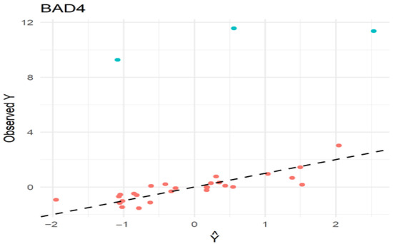
Figure 1. Diagnostic plot of BAD4 estimator (observed vs. predicted values).

The bold value represents the smaller MSE. The simulation results in Table 1, Table 2, Table 3, Table 4 and Table 5 reveal that the BAD estimators (BAD1 to BAD6) demonstrate exceptional robustness against outliers across the varying scenarios presented in the tables. Overall, the BAD estimators maintain low Mean Squared Error (MSE) values, demonstrating superior performance compared to other methods such as OLS, HK, and HKB. Among them, BAD1 and BAD4 consistently yield the lowest MSEs, making them reliable choices—particularly in scenarios with lower confidence levels (0.85 and 0.95) and 10% outliers. As the confidence level increases (up to 0.999) or the percentage of outliers rises to 20%, BAD4 remains especially effective, highlighting its versatility and robustness under extreme conditions. BAD2, BAD3, and BAD5 also perform well, with minimal MSE variation, particularly at higher confidence levels. Although BAD6 shows slightly higher MSE under less extreme conditions, it proves advantageous in cases involving severe outliers and high confidence levels, indicating its suitability for more challenging datasets. In summary, BAD4 emerges as the most robust and versatile estimator overall, while BAD1 is optimal for scenarios with moderate outlier influence. For conditions involving a higher proportion of outliers and stringent confidence requirements, BAD2, BAD5, and BAD6 also deliver strong, reliable performance, making them valuable options for practical applications with noisy data.

The results from Table 5 reveal that, in the case of the heavy-tailed standardized Cauchy distribution, where outliers strongly affect the performance of traditional methods, the BAD estimators consistently demonstrate superior performance by maintaining low Mean Squared Error (MSE) values. Unlike traditional estimators such as OLS, HK, and HKB, which exhibit significantly higher MSE values, especially under high multicollinearity (0.99 and 0.999), the BAD estimators prove to be much more robust. The BAD4 estimator, in particular, achieves remarkably low MSE values even under extreme multicollinearity conditions. These findings highlight the robustness and accuracy of the BAD series in such challenging scenarios, making them a preferable choice when working with heavy-tailed data.

Table 6 provides a bird’s-eye view of all the scenarios explored in the simulation study.

4. Real Life Application

4.1. Tobacco Data

This section includes an empirical case that demonstrates the performance of the novel estimators. We followed [29,30,31] in analyzing tobacco data. The data includes thirty (30) observations of different tobacco mixes. The percentage concentrations of four essential components are employed as predictor variables, with the quantity of heat created by the tobacco during smoking serving as a response variable. The regression model for the tobacco data is shown below.

$$y={\beta }_0+{\beta }_1{X}_1+{\beta }_2{X}_2+{\beta }_3{X}_3+{\beta }_4{X}_4+\epsilon$$

(46)

Figure 2 illustrating the relationships between variables $X_1$, $X_2$, $X_3$, $X_4$, and $y$. The lower triangular matrix displays scatterplots, visualizing the linear relationships between pairs of variables. The upper triangular matrix shows the Pearson correlation coefficients (r), with asterisks (∗∗∗) indicating the strong positive correlation > 0.9. The diagonal panels show the kernel density distribution for each variable. The condition number of this data is obtained as 1855.526, which indicates severe multicollinearity among the predictors. Based on the covariance matrix, observations 4, 18, and 29 are identified as outliers.

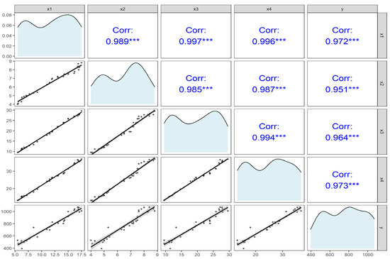
Figure 2. Pairwise correlation between variables of tobacco data of ref. [32].

Table 7 provides a comparative analysis of various regression estimators, including traditional methods like OLS, HK, and HKB, as well as robust estimators such as SH, RM, and the novel BAD series (BAD1 to BAD6), applied to the tobacco dataset. The MSE values indicate the error level for each estimator, with a lower MSE representing better performance.

Table 7. Estimated regression coefficients and MSE values of tobacco data of ref. [32].

Estimators	MSE	$\hat{\mathit{k}}$	${\hat{\mathit{\beta }}}_1$	${\hat{\mathit{\beta }}}_2$	${\hat{\mathit{\beta }}}_3$	${\hat{\mathit{\beta }}}_4$
OLS	32.4972	0.0229	0.4857	−0.6728	1.0744	1.4438
HK	3.6366	0.048619	0.4856	−0.6438	0.9561	1.0548
HKB	3.4022	0.093024	0.4856	−0.6438	0.9561	1.0548
KAM	3.4452	0.067052	0.4856	−0.6438	0.9561	1.0548
KMS	3.6284	0.0229	0.4856	−0.6435	0.9549	1.0515
LC	3.6391	0.0229	0.4867	−0.6453	0.9582	1.0572
ST	3.4095	0.037977	0.2959	0.2242	−0.0961	−0.0394
SH1	3.4286	3.759727	0.487	−0.628	0.8942	0.8987
SH2	3.7361	3.971751	0.4863	−0.0831	0.0521	0.0243
SH3	3.7394	1855.526	0.4863	−0.0793	0.0496	0.023
SH4	3.9102	3.973893	0.4857	−0.0032	0.0018	0.0008
SH5	3.7394	0.002142	0.4863	−0.0792	0.0495	0.023
SH6	12.5412	0.203844	0.4858	−0.6701	1.0624	1.3961
RM	6.9082	20.18056	0.4888	−0.65	1.232	0.8844
BAD1	2.5162	21.31861	0.491	−0.4672	0.5899	0.2078
BAD2	2.8615	9959.644	0.489	−0.0188	0.0132	0.0032
BAD3	2.8647	21.3301	0.489	−0.018	0.0126	0.003
BAD4	2.9447	0.011495	0.4888	−0.0029	0.002	0.0005
BAD5	2.8647	0.0229	0.489	−0.018	0.0126	0.003
BAD6	1.7834	0.048619	0.4893	−0.6364	1.1613	0.7471

Note: Bold values show the minimum MSE of estimators.

The results highlight the limitations of traditional methods like OLS, which has the highest MSE (32.4972), suggesting poor robustness against multicollinearity and outliers. On the other hand, the novel BAD estimators demonstrate significantly lower MSE values. In particular, BAD6 achieves the lowest MSE (1.7834), indicating superior performance and robustness, especially in handling the severe multicollinearity and outliers present in the tobacco data. This is further supported by the regression coefficients, where BAD6 shows consistent and stable values.

BAD1, BAD3, and BAD4 also exhibit strong performance, with MSE values of 2.5162, 2.8647, and 2.9447, respectively, indicating their effectiveness as well. Notably, BAD4 achieves the lowest regression coefficient estimates, suggesting high precision and stability.

The robust performance of BAD6, followed closely by BAD1 and BAD4, suggests that these novel estimators provide a reliable alternative to traditional methods, particularly in datasets affected by multicollinearity and outliers. The bolded values indicate the estimators with the minimum MSE, further emphasizing the effectiveness of BAD estimators in this empirical case study.

To compare the statistical properties of estimators, the 95% CI was computed for each regression coefficient ${\hat{\beta }}_i=(i=0,1,2,3,4)$ under OLS, ridge regression, robust ridge, and two-parameter robust ridge regression. The confidence intervals were constructed using asymptotic variance–covariance matrices. The variance–covariance matrix for OLS is given by

$$Var({\hat{\beta }}_{OLS})={\hat{\sigma }}^2{(X\prime X)}^{-1}$$

(47)

and for RR, by

$$Var({\hat{\beta }}_{RR})={\hat{\sigma }}^2{(X\prime X+kI)}^{-1}(X\prime X){(X\prime X+kI)}^{-1}$$

(48)

The standard errors (SE) were obtained from the diagonal elements of these matrices, and the 95% CIs were obtained as follows:

$$CI={\hat{\beta }}_i\pm t_{1-(\alpha /2),n-p}\left(\sqrt{Var({\hat{\beta }}_i)}\right)$$

(49)

where $t_{(1-{\displaystyle \raisebox{1ex}{$\alpha $}\!\left/ \!\raisebox{-1ex}{$2$}\right.})}$, is the $(1-{\displaystyle \raisebox{1ex}{$\alpha $}\!\left/ \!\raisebox{-1ex}{$2$}\right.})$ quantile of Student’s t-distribution with n − 1 degrees of freedom.

The 95% CIs for the predictors are presented in Table 8. We denote $L({\hat{\beta }}_i)$ and $U({\hat{\beta }}_i)$ as the lower and upper bounds of the confidence interval, respectively [10].

Table 8. Confidence intervals (95%) for tobacco data.

Estimator	$\mathbf{L}({\hat{\mathit{\beta }}}_1)$	$\mathbf{U}({\hat{\mathit{\beta }}}_1)$	$\mathbf{L}({\hat{\mathit{\beta }}}_2)$	$\mathbf{U}({\hat{\mathit{\beta }}}_2)$	$\mathbf{L}({\hat{\mathit{\beta }}}_3)$	$\mathbf{U}({\hat{\mathit{\beta }}}_3)$	$\mathbf{L}({\hat{\mathit{\beta }}}_4)$	$\mathbf{U}({\hat{\mathit{\beta }}}_4)$
OLS	0.005905409	3.00888230	−1.081589605	0.03945686	−1.939348004	0.25614058	−0.158615271	1.80203453
HK	0.086753653	2.2905041	−0.992556171	0.0693747	−1.472925571	0.2829355	0.002113015	1.6676833
HKB	0.13701839	1.83847598	−0.91527338	0.09201028	−1.15820596	0.30739028	0.09383117	1.53919381
KAM	0.1830328	1.4101702	−0.8106986	0.1178389	−0.8334673	0.3345412	0.1710530	1.3623161
KMS	0.087449377	2.28429487	−0.991640189	0.06966175	−1.468742092	0.28323228	0.003428956	1.66620587
LC	0.086753653	2.2905041	−0.992556171	0.0693747	−1.472925571	0.2829355	0.002113015	1.6676833
ST	0.086753653	2.2905041	−0.992556171	0.0693747	−1.472925571	0.2829355	0.002113015	1.6676833
SH1	0.11945717	1.9974122	−0.94523488	0.0836136	−1.27146581	0.2981569	0.06258856	1.5897296
SH2	0.23338782	0.3065626	0.09152924	0.2272470	0.17599167	0.2728077	0.23910454	0.3340377
SH3	0.23255299	0.3031387	0.09761709	0.2274706	0.17824594	0.2710924	0.23811747	0.3291206
SH4	0.01307684	0.01553164	0.01275406	0.01521052	0.01296331	0.01541858	0.01309625	0.01555145
SH5	0.23254468	0.3031058	0.09767539	0.2274726	0.17826721	0.2710757	0.23810770	0.3290733
SH6	0.01593272	2.91995177	−1.07199693	0.04285575	−1.88313513	0.25867334	−0.13789222	1.78860732
RM	0.00590541	3.00888230	−1.08158961	0.03945686	−1.93934800	0.25614058	−0.15861527	1.80203453
BAD1	0.2258518	0.9607248	−0.6281803	0.1526566	−0.4481616	0.3590181	0.2352873	1.0772170
BAD2	0.1950698	0.2326699	0.1683647	0.2127897	0.1852614	0.2249406	0.1973076	0.2366952
BAD3	0.1932249	0.2303480	0.1679842	0.2113445	0.1839646	0.2229785	0.1953685	0.2341155
BAD4	0.00255732	0.00303745	0.00249660	0.00297679	0.00253601	0.00301615	0.00256080	0.00304094
BAD5	0.1932065	0.2303250	0.1679798	0.2113299	0.1839515	0.2229589	0.1953492	0.2340901
BAD6	0.05284466	2.59234445	−1.03357815	0.05606784	−1.67271552	0.26987847	−0.06347370	1.73209874

In Table 8, where the CI values are presented, it is clear that traditional estimators such as OLS, HK, HKB, LC, and RM exhibit wide ranges, reflecting higher variability and lower precision. KAM and KMS provide somewhat narrower bounds, with KMS showing improved stability compared to OLS. The shrinkage-type estimators (ST, SH1–SH6) considerably reduce interval widths, with SH2–SH5 in particular producing highly compact bounds that suggest strong reliability. Most notably, the BAD family (BAD1–BAD6) achieves the narrowest intervals overall, with BAD4 displaying the smallest and most consistent ranges across all coefficients, marking it as the most precise and stable estimator among those compared.

Figure 3 illustrates a response plot using the BAD4 estimator. It shows the relationship between the fitted values (predicted values) and the observed values of a variable Y. The x-axis represents the fitted values ($\hat{Y}$) from BAD4, which are the predicted values from a statistical model using a BAD4 estimator. The y-axis represents the observed Y, which are the actual data points. The plot illustrates how well the BAD4 estimator fits the data while highlighting potential outliers. Most points (blue) align with the model’s predictions, indicating a good overall fit. One point’s X-outlier (orange) stands out with unusually high leverage. This diagnostic tool helps to visually identify influential observations that may affect model performance.

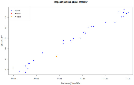
Figure 3. Diagnosis of influential observation and BAD4 estimator.

4.2. Gasoline Consumption Data

To further evaluate the performance of the proposed estimators under severe multicollinearity with y-direction outliers, the Gasoline Consumption dataset was analyzed [33]. This dataset comprises 30 automobile models, with fuel consumption (miles per gallon, y) as the response variable and four predictors: displacement (X₁), horsepower (X₂), torque (X₃), and width (X₄). The linear regression model is expressed as follows:

$$y={\beta }_0+{\beta }_1{X}_1+{\beta }_2{X}_2+{\beta }_3{X}_3+{\beta }_4{X}_4+\epsilon$$

(50)

The eigen values (λ₁ = 3.606, λ₂ = 0.335, λ₃ = 0.052, λ₄ = 0.007) yield a condition number of 531.128 and a condition index of 23.046, confirming severe multicollinearity. Outlier detection using Cook’s distance identified observations 8 and 24 (values 0.01 and 0.00, respectively) as having negligible influence on regression estimates. Correlation analysis (Figure 4) revealed strong positive associations among predictors, while gasoline consumption showed a moderate negative relationship with all explanatory variables.

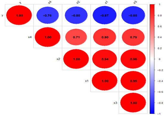
Figure 4. Pairwise correlation between variables of gasoline consumption data.

The results in Table 8 demonstrate that the proposed estimators significantly outperform OLS and RM, which yield very high MSE values (41.67 and 43.39, respectively), indicating poor predictive accuracy under multicollinearity and outliers. In contrast, estimators such as BAD2 (MSE = 1.9266), BAD3 (MSE = 1.9338), and BAD5 (MSE = 1.9339) achieve the lowest MSE values, demonstrating superior efficiency.

Table 9 below demonstrates that in the case of severe multicollinearity along with outliers, as in the gasoline consumption data, all the BAD estimators perform well compared to other traditional and newly developed TPREs, among which the BAD2 estimator outperforms all the others with a lower MSE; the same results are presented in a bar chart (Figure 5).

Table 9. Estimated regression coefficients and MSE of gasoline consumption data.

Estimators	MSE	$\hat{\mathit{k}}$	${\hat{\mathit{\beta }}}_1$	${\hat{\mathit{\beta }}}_2$	${\hat{\mathit{\beta }}}_3$	${\hat{\mathit{\beta }}}_4$
OLS	41.6654	---	−1.3852	−0.0776	0.7395	−0.1818
HK	2.8849	0.125136	−1.0441	0.0062	0.3216	−0.1841
HKB	2.4426	0.391949	−0.7742	0.0343	0.0345	−0.192
KAM	2.4143	11.0074	−0.265	−0.1474	−0.2048	−0.206
KMS	2.6778	0.180161	−0.9613	0.0201	0.2275	−0.1857
LC	2.8957	0.125136	−1.0513	0.0062	0.3238	−0.1854
ST	2.3682	0.125136	0.4766	−0.6728	0.093	−0.2518
SH1	5.2235	0.029569	−1.2763	−0.0468	0.5998	−0.1825
SH2	2.3456	2.927352	−0.4054	−0.0778	−0.2043	−0.2255
SH3	2.3522	3.59956	−0.3809	−0.0942	−0.2108	−0.2275
SH4	2.4876	531.1282	−0.243	−0.2195	−0.2354	−0.2124
SH5	2.3523	3.60635	−0.3807	−0.0943	−0.2108	−0.2275
SH6	14.0126	0.00679	−1.3577	−0.0695	0.7039	−0.1819
RM	43.3854	---	−1.2593	−0.0761	0.6094	−0.1586
BAD1	2.1431	0.230061	−0.8418	0.013	0.108	−0.1658
BAD2	1.9266	22.77608	−0.2618	−0.1912	−0.2292	−0.2112
BAD3	1.9338	28.00615	−0.2573	−0.1958	−0.2296	−0.2106
BAD4	1.9738	4132.409	−0.2373	−0.2178	−0.2317	−0.2054
BAD5	1.9339	28.05898	−0.2572	−0.1958	−0.2297	−0.2106
BAD6	3.6023	0.052829	−1.1027	−0.0342	0.4113	−0.16

Bold values show the minimum MSE of estimators.

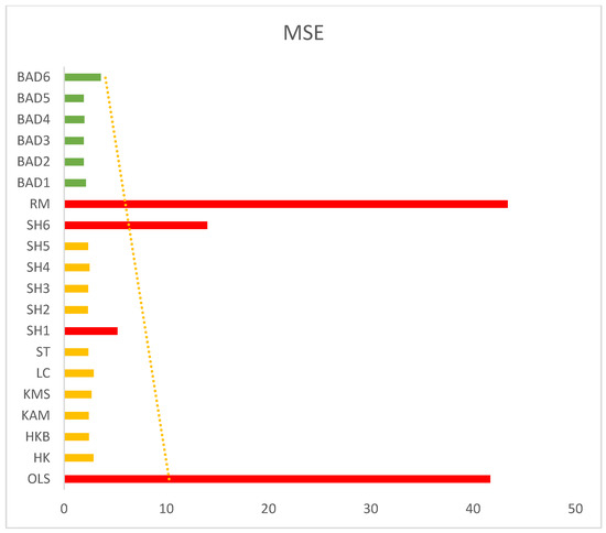
Figure 5. Estimated MSE of OLS, RR, TPRR, and TPRRE on gasoline consumption data.

Table 10 present the 95% CI results for the proposed estimator, and demonstrate that the most striking results come from the BAD estimators (BAD1–BAD6), which consistently generate extremely narrow and stable confidence intervals. Among them, BAD4 demonstrates the smallest and most uniform ranges for all coefficients, establishing it as the most precise and reliable estimator for the gasoline consumption data.

Table 10. Confidence intervals (95%) for gasoline consumption data.

Estimator	$\mathbf{L}({\hat{\mathit{\beta }}}_1)$	$\mathbf{U}({\hat{\mathit{\beta }}}_1)$	$\mathbf{L}({\hat{\mathit{\beta }}}_2)$	$\mathbf{U}({\hat{\mathit{\beta }}}_2)$	$\mathbf{L}({\hat{\mathit{\beta }}}_3)$	$\mathbf{U}({\hat{\mathit{\beta }}}_3)$	$\mathbf{L}({\hat{\mathit{\beta }}}_4)$	$\mathbf{U}({\hat{\mathit{\beta }}}_4)$
OLS	−2.8055562	0.03505633	−0.8672192	0.71210810	−1.0835724	2.56266260	−0.5072373	0.14366063
HK	−1.9825876	−0.1055709	−0.6418893	0.6542284	−0.8043292	1.4475464	−0.5008870	0.1327180
HKB	−1.3771884	−0.1712334	−0.4905127	0.5591917	−0.5980824	0.6671426	−0.4939614	0.1099976
KAM	−0.3487039	−0.18136093	−0.2543979	−0.04044512	−0.2747117	−0.13486242	−0.3469731	−0.06510444
KMS	−0.8061589	−0.18855485	−0.3582714	0.31477895	−0.4132073	0.08948395	−0.4736704	0.05204371
LC	−0.9645881	−0.18691899	−0.3937764	0.40638817	−0.4623507	0.22131849	−0.4830179	0.07408722
ST	−1.7915100	−0.1311066	−0.5928314	0.6331199	−0.7391093	1.1940173	−0.4991013	0.1277443
SH1	−1.9825876	−0.1055709	−0.6418893	0.6542284	−0.8043292	1.4475464	−0.5008870	0.1327180
SH2	−1.9825876	−0.1055709	−0.6418893	0.6542284	−0.8043292	1.4475464	−0.5008870	0.1327180
SH3	−0.5420450	−0.18992433	−0.3014015	0.12048930	−0.3352603	−0.06977346	−0.4357091	−0.00148512
SH4	−0.04862990	−0.03127241	−0.04484962	−0.02730786	−0.04736591	−0.03003570	−0.04395334	−0.02587430
SH5	−0.5415998	−0.18992344	−0.3013062	0.12012548	−0.3351310	−0.06997787	−0.4355971	−0.00160123
SH6	−2.7351129	0.02166785	−0.8470784	0.70808765	−1.0597851	2.46656350	−0.5067362	0.14312908
RM	−2.8055562	0.03505633	−0.8672192	0.71210810	−1.0835724	2.56266260	−0.5072373	0.14366063
BAD1	−1.6971556	−0.14224850	−0.5690558	0.62040530	−0.7068929	1.07056110	−0.4981252	0.12469070
BAD2	−0.2815145	−0.16555419	−0.2274766	−0.08380654	−0.2441799	−0.13846204	−0.2835324	−0.08844829
BAD3	−0.2636527	−0.15873567	−0.2179411	−0.09060437	−0.2336887	−0.13602504	−0.2636417	−0.09219561
BAD4	−0.00777730	−0.00500441	−0.00721815	−0.00444137	−0.00760737	−0.00483503	−0.00698284	−0.00419447
BAD5	−0.2634937	−0.15866962	−0.2178510	−0.09065279	−0.2335898	−0.13599593	−0.2634617	−0.09222115
BAD6	−2.3824579	−0.04213433	−0.7485814	0.68629135	−0.9403875	1.98667893	−0.5041413	0.13955386

5. Some Concluding Remarks

This study presented a comparative analysis of traditional regression estimators (OLS), one-parameter ridge estimators and recently proposed two-parameter ridge estimators (SH1–SH6), traditional robust ridge, and a novel class of Two-Parameter Robust Ridge M-Estimators (BAD1–BAD6). Both simulation experiments and real-life datasets (Tobacco and Gasoline Consumption) were used to evaluate performance, with MSE serving as the primary criterion. The findings demonstrate that OLS is highly sensitive to multicollinearity and outliers, producing unstable and inefficient estimates under such conditions. Recently developed two-parameter ridge estimators improved estimation accuracy over classical ridge forms by introducing an additional shrinkage parameter, yet they remain vulnerable to extreme data contamination. Robust ridge estimators demonstrated resilience to outliers, but were less efficient under severe multicollinearity. In contrast, the proposed BAD series of Two-Parameter Robust Ridge M-Estimators successfully integrates the dual benefits of robustness and efficiency. Specifically, BAD2, BAD4, and BAD6 consistently achieved the lowest MSE values across diverse scenarios, showing greater stability compared to both earlier two-parameter ridge estimators and robust single-parameter methods. These results provide justification for the theoretical superiority and practical utility of the proposed class.

References

- Mao, S. Statistical Derivation of Linear Regression. In International Conference on Statistics, Applied Mathematics, and Computing Science (CSAMCS 2021); SPIE: Bellingham, WA, USA, 2022; Volume 12163, pp. 893–901. [Google Scholar]
- Maulud, D.; Abdulazeez, A.M. A Review on Linear Regression Comprehensive in Machine Learning. J. Appl. Sci. Technol. Trends 2020, 1, 140–147. [Google Scholar] [CrossRef]
- Lukman, A.F.; Mohammed, S.; Olaluwoye, O.; Farghali, R.A. Handling Multicollinearity and Outliers in Logistic Regression Using the Robust Kibria–Lukman Estimator. Axioms 2024, 14, 19. [Google Scholar] [CrossRef]
- Lukman, A.F.; Jegede, S.L.; Bellob, A.B.; Binuomote, S.; Haadi, A. Modified Ridge-Type Estimator with Prior Information. Int. J. Eng. Res. Technol. 2019, 12, 1668–1676. [Google Scholar]
- Hoerl, A.E.; Kennard, R.W. Ridge Regression: Biased Estimation for Nonorthogonal Problems. Technometrics 1970, 12, 55–67. [Google Scholar] [CrossRef]
- Mermi, S.; Göktaş, A.; Akkuş, Ö. How Well Do Ridge Parameter Estimators Proposed so Far Perform in Terms of Normality, Outlier Detection, and MSE Criteria? Commun. Stat. Comput. 2024. [Google Scholar] [CrossRef]
- Lipovetsky, S.; Conklin, W.M. Ridge Regression in Two-Parameter Solution. Appl. Stoch. Model. Bus. Ind. 2005, 21, 525–540. [Google Scholar] [CrossRef]
- Toker, S.; Kaçiranlar, S. On the Performance of Two Parameter Ridge Estimator under the Mean Square Error Criterion. Appl. Math. Comput. 2013, 219, 4718–4728. [Google Scholar] [CrossRef]
- Abdelwahab, M.M.; Abonazel, M.R.; Hammad, A.T.; El-Masry, A.M. Modified Two-Parameter Liu Estimator for Addressing Multicollinearity in the Poisson Regression Model. Axioms 2024, 13, 46. [Google Scholar] [CrossRef]
- Alharthi, M.F.; Akhtar, N. Modified Two-Parameter Ridge Estimators for Enhanced Regression Performance in the Presence of Multicollinearity: Simulations and Medical Data Applications. Axioms 2025, 14, 527. [Google Scholar] [CrossRef]
- Shakir, M.; Ali, A.; Suhail, M.; Sadun, E. On the Estimation of Ridge Penalty in Linear Regression: Simulation and Application. Kuwait J. Sci. 2024, 51, 100273. [Google Scholar] [CrossRef]
- Khan, M.S. Adaptive Penalized Regression for High-Efficiency Estimation in Correlated Predictor Settings: A Data-Driven Shrinkage Approach. Mathematics 2025, 13, 2884. [Google Scholar] [CrossRef]
- Silvapulle, M.J. Robust Ridge Regression Based On An M-Estimator. Austral. J. Stat. 1991, 33, 319–333. [Google Scholar]
- Hoerl, A.E.; Kannard, R.W.; Baldwin, K.F. Ridge Regression: Some Simulations. Commun. Stat. Methods 1975, 4, 105–123. [Google Scholar] [CrossRef]
- Lawless, J.F.; Wang, P. A Simulation Study Of Ridge And Other Regression Estimators. Commun. Stat.—Theory Methods 1976, 5, 307–323. [Google Scholar] [CrossRef]
- Begashaw, G.B.; Yohannes, Y.B. Review of Outlier Detection and Identifying Using Robust Regression Model. Int. J. Syst. Sci. Appl. Math. 2020, 5, 4–11. [Google Scholar] [CrossRef]
- Majid, A.; Ahmad, S.; Aslam, M.; Kashif, M. A Robust Kibria–Lukman Estimator for Linear Regression Model to Combat Multicollinearity and Outliers. Concurr. Comput. Pract. Exp. 2023, 35, e7533. [Google Scholar] [CrossRef]
- Suhail, M.; Chand, S.; Aslam, M. New Quantile Based Ridge M-Estimator for Linear Regression Models with Multicollinearity and Outliers. Commun. Stat. Simul. Comput. 2023, 52, 1418–1435. [Google Scholar] [CrossRef]
- Wasim, D.; Suhail, M.; Albalawi, O.; Shabbir, M. Weighted Penalized M-Estimators in Robust Ridge Regression: An Application to Gasoline Consumption Data. J. Stat. Comput. Simul. 2024, 94, 3427–3456. [Google Scholar] [CrossRef]
- Ertaş, H.; Toker, S.; Kaçıranlar, S. Robust Two Parameter Ridge M-Estimator for Linear Regression. J. Appl. Stat. 2015, 42, 1490–1502. [Google Scholar] [CrossRef]
- Yasin, S.; Salem, S.; Ayed, H.; Kamal, S.; Suhail, M.; Khan, Y.A. Modified Robust Ridge M-Estimators in Two-Parameter Ridge Regression Model. Math. Probl. Eng. 2021, 2021, 1845914. [Google Scholar] [CrossRef]
- Wasim, D.; Khan, S.A.; Suhail, M. Modified Robust Ridge M-Estimators for Linear Regression Models: An Application to Tobacco Data. J. Stat. Comput. Simul. 2023, 93, 2703–2724. [Google Scholar] [CrossRef]
- Huber, P.J. Robust Statistical Procedures; SIAM: Philadelphia, PA, USA, 1996. [Google Scholar]
- Hoerl, A.E.; Kennard, R.W. Ridge Regression: Applications to Nonorthogonal Problems. Technometrics 1970, 12, 69–82. [Google Scholar] [CrossRef]
- Kibria, B.M.G. Performance of Some New Ridge Regression Estimators. Commun. Stat. Part B Simul. Comput. 2003, 32, 419–435. [Google Scholar] [CrossRef]
- Khalaf, G.; Mansson, K.; Shukur, G. Modified Ridge Regression Estimators. Commun. Stat.—Theory Methods 2013, 42, 1476–1487. [Google Scholar] [CrossRef]
- Dar, I.S.; Chand, S.; Shabbir, M.; Kibria, B.M.G. Condition-Index Based New Ridge Regression Estimator for Linear Regression Model with Multicollinearity. Kuwait J. Sci. 2023, 50, 91–96. [Google Scholar] [CrossRef]
- Ali, A.; Suhail, M.; Awwad, F.A. On the Performance of Two-Parameter Ridge Estimators for Handling Multicollinearity Problem in Linear Regression: Simulation and Application. AIP Adv. 2023, 13, 115208. [Google Scholar] [CrossRef]
- Ertaş, H. A Modified Ridge M-Estimator for Linear Regression Model with Multicollinearity and Outliers. Commun. Stat. Simul. Comput. 2018, 47, 1240–1250. [Google Scholar] [CrossRef]
- Suhail, M.; Chand, S.; Kibria, B.M.G. Quantile-Based Robust Ridge m-Estimator for Linear Regression Model in Presence of Multicollinearity and Outliers. Commun. Stat. Simul. Comput. 2021, 50, 3194–3206. [Google Scholar] [CrossRef]
- Wasim, D.; Khan, S.A.; Suhail, M.; Shabbir, M. New Penalized M-Estimators in Robust Ridge Regression: Real Life Applications Using Sports and Tobacco Data. Commun. Stat. Simul. Comput. 2025, 54, 1746–1765. [Google Scholar] [CrossRef]
- Myers, R.H.; Sliema, B. Classical and Modern Regression with Applications; Duxbury Thomson Learning: Pacific Grove, CA, USA, 1990. [Google Scholar]
- Babar, I.; Ayed, H.; Chand, S.; Suhail, M.; Khan, Y.A.; Marzouki, R. Modified Liu Estimators in the Linear Regression Model: An Application to Tobacco Data. PLoS ONE 2021, 16, e0259991. [Google Scholar] [CrossRef]
Disclaimer/Publisher’s Note: The statements, opinions and data contained in all publications are solely those of the individual author(s) and contributor(s) and not of MDPI and/or the editor(s). MDPI and/or the editor(s) disclaim responsibility for any injury to people or property resulting from any ideas, methods, instructions or products referred to in the content. |
© 2025 by the authors. Licensee MDPI, Basel, Switzerland. This article is an open access article distributed under the terms and conditions of the Creative Commons Attribution (CC BY) license (https://creativecommons.org/licenses/by/4.0/).