Article

Pattern Classification for Mixed Feature-Type Symbolic Data Using Supervised Hierarchical Conceptual Clustering

School of Science and Engineering, Tokyo Denki University, Hatoyama, Saitama 350-0394, Japan
*
Author to whom correspondence should be addressed.
Stats 2025, 8(3), 76; https://doi.org/10.3390/stats8030076
Submission received: 5 July 2025 / Revised: 7 August 2025 / Accepted: 8 August 2025 / Published: 25 August 2025

Abstract

This paper describes a region-oriented method of pattern classification based on the Cartesian system model (CSM), a mathematical model that allows manipulating mixed feature-type symbolic data. We use the supervised hierarchical conceptual clustering to generate class regions for respective pattern class based on the evaluation of the generality of the regions and the separability of the regions against other classes in each clustering step. We can easily find the robustly informative features to describe each pattern class against other pattern classes. Some examples show the effectiveness of the proposed method.

1. Introduction

Feature selection has been extensively developed in pattern recognition, data mining [1,2,3], and, more generally, symbolic data analysis [4]. Feature selection has two main problems: how to evaluate the importance of the given features and how to find a set of important feature subset from the given set of features. As summarized in [1,2,3,5], many feature selection methods have been developed by combining various feature evaluation measures (distance measure, information measure, dependency measure, consistency measure, and classification error rate) and search strategies (heuristic, complete, and random).
The authors reported an unsupervised feature selection method using the hierarchical conceptual clustering for histogram-valued symbolic data [6]. In this method, each object is described by a series of quantile vectors, and the concept size, called the compactness, is used as the similarity measure between objects and/or clusters represented by the quantile vectors. It should be noted that the compactness also plays the roles of cluster quality criterion and feature-effectiveness criterion. This fact simplifies the process of unsupervised feature selection.
As a pattern classifier for mixed feature-type symbolic data, the authors proposed region-oriented method based on the Cartesian system model (CSM) [7], where the authors pointed out the trade-off between the "separability" of classes and the "generality" of class descriptions, and asserted the importance of feature selection.
The purpose of this paper is to realize a feature selection method for our region-oriented classifier using the supervised hierarchical conceptual clustering.
In Section 2, the CSM is defined by the triplet (D(d), ⊞, ⊠), where D(d) is the feature space composed of d mixed-type features. We define the Cartesian join operator ⊞ and the Cartesian meet operator ⊠ on the feature space. The Cartesian join generates a generalized description of the given two descriptions in the feature space. On the other hand, the Cartesian meet extracts a common description from the given two descriptions in the feature space. We define the measure of compactness with respect to the Cartesian join in order to evaluate the generality of cluster descriptions in each clustering step. Subsection 2.2 describes the algorithm of our unsupervised hierarchical conceptual clustering using the compactness. Subsection 2.3 describes our classification model based on the supervised hierarchical conceptual clustering. This clustering algorithm checks, in each clustering step, not only the generality of the class description but also the separability of the class description against other pattern classes using the Cartesian meet operator.
Section 3 describes three experimental results in order to show the effectiveness of the proposed method. Section 4 discusses the obtained results.

2. Cartesian System Model (CSM) and Feature Selection Using Hierarchical Conceptual Clustering

In this section, we describe the Cartesian system model, a mathematical model for mixed feature-type symbolic data. We define a measure to evaluate the compactness of the generated concepts, and we describe an algorithm of the unsupervised hierarchical conceptual clustering. Then, we describe the classification model based on the supervised hierarchical conceptual clustering.

2.1. The Cartesian System Model (CSM)

Let Dk be the domain of feature Fk, k =1, 2, …, d. Then, the feature space is defined by
D(d)= D1 × D2 × ⋯ × Dd.
Since we permit the simultaneous use of various feature types, we use the notation D(d) for the feature space in order to distinguish it from usual d-dimensional Euclidean space Dd. Each element of D(d) is represented by
E = E1 × E2 × ⋯ × Ed or E = (E1, E2, …, Ed).
where Ek is the feature value taken by the feature Fk, k = 1, 2, …, d. We are able to use the following feature types:
(1)
Continuous quantitative feature (e.g., height and weight);
(2)
Discrete quantitative feature (e.g., the number of family members);
(3)
Ordinal qualitative feature (e.g., academic career, etc., where there is some kind of ordered relationships between values)
(4)
Nominal qualitative feature (e.g., gender and blood type).
When we use feature types (1), (2), and (3), we permit interval values of the form Ek = [a, b], and in the case of feature type (4), we allow for finite sets as feature values. The Cartesian product (2) described in terms of feature types (1)–(4) is called an event in the feature space D(d).

2.1.1. The Cartesian Join Operator

The Cartesian join, AB, of a pair of events A = (A1, A2, …, Ad) and B = (B1, B2, …, Bd) in the feature space D(d), is defined by
AB = [A1B1] × [A2B2] × ⋯ × [AdBd],
where [AkBk] is the Cartesian join of feature values Ak and Bk for feature Fk and is defined as follows.
When Fk is a quantitative or an ordinal qualitative feature, let Ak = [AkL, AkU] and Bk = [BkL, BkU], then [AkBk] is the closed interval given by
[Ak⊞Bk] = [min(AkL, BkL), max(AkU, BkU)].
When Fk is a nominal feature, [AkBk] is the union:
[AkBk] = AkBk.
Figure 1a illustrates the Cartesian join of two interval-valued events A and B in the Euclidean plane.

2.1.2. The Cartesian Meet Operator

The Cartesian meet AB of a pair of events A = (A1, A2, …, Ad) and B = (B1, B2, …, Bd) in the feature space D(d) is defined by
AB = [A1B1] × [A2B2] × ⋯ × [AdBd],
where [AkBk] is the Cartesian meet of feature values Ak and Bk for feature Fk defined by the intersection:
[Ak⊠Bk] = Ak ∩ Bk.
When the intersection (7) takes the empty value ∅, for at least one feature, the events A and B have no common part. We denote this fact by
AB = ,
and we say that A and B are completely distinguishable. Figure 1b illustrates the Cartesian meet of two interval-valued events, A and B. We call the triplet (D(d), ⊞, ⊠) the Cartesian System Model (CSM).

2.1.3. Concept Size

Let U = {ω1, ω2, …, ωN} be the given set of sample objects without class labels, and let each sample object ωk be described by an event Ek = Ek1 × Ek2 × ⋯ × Ekd in D(d). We define the concept size P(Ekj) of ωk in terms of feature Fj as the probability:
P(Ekj) = |Ekj|/|Dj|, j = 1, 2, …, d; k = 1, 2, …, N, and
0 ≤ P(Ekj) ≤ 1, j = 1, 2, …, d; k = 1, 2, …, N,
where |Dj| is the length of the interval Dj, if feature Fj is type (1), (2), or (3) in Section 2.1, and is the number of elements in the set Dj if feature Fj is type (4). Then, we define the concept size P(Ek) of ωk in the feature space D(d) by the arithmetic mean:
P(Ek) = {P(Ek1) + P(Ek2) + ⋯ + P(Ekd)}/d, and
0 ≤ P(Ek) ≤ 1, k = 1, 2, …, N.

2.2. Measure of Compactness and Unsupervised Hierarchical Conceptual Clustering

2.2.1. Measure of Compactness

In the CSM, each sample object ωp is described as an event Ep which is equivalent to a conjunctive logical expression and is regarded as a minimum unit of concept described by d features. Now, we define the measure of compactness for the concept generated by two sample objects ωp and ωq, written C(ωp, ωq), as follows:
C(ωp, ωq) = P(EpEq) = {P(Ep1Eq1) + P(Ep2Eq2) + ⋯ + P(EpdEqd)}/d.
Since the Cartesian join EpEq generates the smallest description spanned by the given two events Ep and Eq, the compactness C(ωp, ωq) evaluates the quantitative size of the generated “concept”. The compactness satisfies the following properties:
(1)
0 ≤ Cp, ωq) ≤ 1;
(2)
C(ωp, ωp) = P(Ep) ≥ 0;
(3)
C(ωp, ωq) = C(ωq, ωp);
(4)
C(ωp, ωq) = 0 iff EiEl and has null size (P(Ei) = 0);
(5)
C(ωp, ωp), C(ωq, ωq) ≤ C(ωp, ωq);
(6)
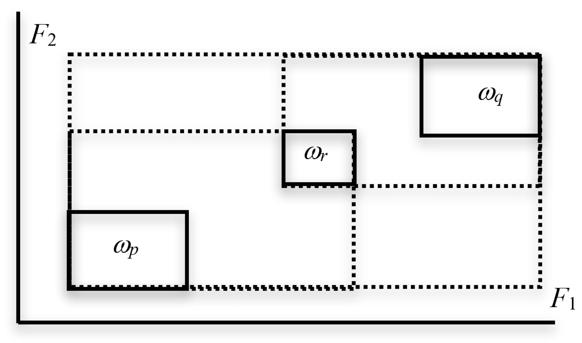
The triangle law C(ωp, ωq) ≤ C(ωp, ωr) + C(ωr, ωq) may not hold as in Figure 2.

2.2.2. Unsupervised Hierarchical Conceptual Clustering

Let U = {ω1, ω2, …, ωN} be the given set of sample objects, and let each ωk be described by an event Ek = Ek1 × Ek2 × ⋯ × Ekd in the feature space D(d). By using the measure of compactness defined in (13), we can construct the following algorithm [6].
Algorithm of the unsupervised hierarchical conceptual clustering:
Step (1)
For each pair of sample objects ω and ω’ in U, calculate the compactness C(ω, ω’) in (13) and find the pair ωp and ωq that has the minimum compactness.
Step (2)
Generate the merged concept ωpq of ωp and ωq in U, and replace ωp and ωq in U by the new concept ωpq, where ωpq is described by the Cartesian join Epq = EpEq in the feature space D(d).
Step (3)
Repeat Step 2 until U includes only one concept (i.e., the whole concept generated by the given N sample objects). (End of Algorithm)
In the above algorithm, Step 1 finds the most similar sample objects and/or sub-concepts that should be merged into a single concept, and then Step 2 characterizes a new extensional concept by the Cartesian join region, which is equivalent to a conjunctive logical expression. Since minimizing the concept size of the Cartesian join region means to maximize the dissimilarity of the join region from the whole region D(d), the compactness plays the role of the cluster quality criterion. We should also note the fact that through the steps of agglomeration process, we can know not only the sizes of sub-concepts but also which features create the differences between sub-concepts. Therefore, the compactness also plays the role of the feature-effectiveness criterion.
As an illustrative example, we apply our unsupervised hierarchical conceptual clustering to the data in Table 1, where each sample is described by five features:
(1)
Specific gravity,
(2)
Freezing point (°C),
(3)
Iodine value,
(4)
Saponification value,
(5)
Major acids.
Figure 3 shows the results for two selected informative features: iodine value and specific gravity. We have three explicit clusters: linseed and perilla; cotton, sesame, olive, and camellia; and beef and hog. These three clusters take similar concept-size values for the selected two features.
Table 1. Fats and oils data [6].
SampleSpecific G.Freezing P.Iodine V.Saponification V.Major Acids
Linseed[0.930, 0.935][−27, −18][170, 204][118, 196][1.75, 4.81]
Perilla[0.930, 0.937][−5, −4][192, 208][188, 197][0.77, 4.85]
Cotton[0.916, 0.918][−6, −1][99, 113][189, 198][0.42, 3.84]
Sesame[0.920, 0.926][−6,−4][104, 116][187, 193][0.91, 3.77]
Camellia[0.916, 0.917][−21, −15][80, 82][189, 193][2.00, 2.98]
Olive[0.914, 0.919][0, 6][79, 90][187, 196][0.83, 4.02]
Beef[0.860, 0.870][30, 38][40, 48][190, 199][0.31, 2.89]
Hog[0.858, 0.864][22, 32][53, 77][190, 202][0.37, 3.65]

2.3. Classification Model Based on the Supervised Conceptual Clustering

In this subsection, we describe a classification model, and we use the term “sample pattern” when referring to a sample object.

2.3.1. Classification Model

Let C1, C2, …, CM be M pattern classes and, for each pattern class Ck, let
Uk = {ωk1, ωk2, …, ωkNk}, k = 1, 2, …, M
be the given set of Nk sample patterns for class Ck. Let each sample pattern ωkj in class Ck be represented in the d-dimensional feature space D(d) as follows:
Ekj = Ekj1 × Ekj2 × ⋯ × Ekjd, j = 1, 2, …, Nk; k = 1, 2, …, M.
From the consistency viewpoint, we assume that, for any pair of p and q (≠ p), Up and Uq have no common sample patterns:
UpUq = ∅.
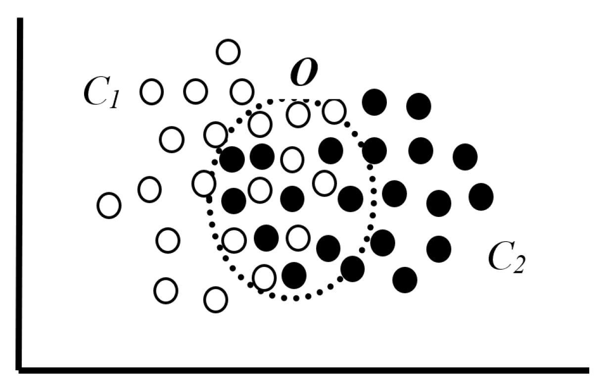
This condition, however, does not mean that two pattern classes share the disjoint regions in the feature space D(d). For example, in Figure 4, two pattern classes share an overlapped region O, but the training sets do not have any common sample pattern.
We use the term subclass for a subset of sample patterns from a pattern class. A subclass of a pattern class is described by a closed region in the feature space D(d). A closed region for a subclass is reduced to a hyper box when the feature space D(d) is a Euclidean space. Moreover, a sample pattern given as a point in the feature space D(d) is also regarded as a closed region that describes a subclass.
Now, let Ωkp and Rkp, p =1, 2, …, mk (≤Nk), be mk subsets of the training set Uk, i.e., subclasses of class Ck, and their representation in the feature space D(d), respectively, such that
Ekp⊆ (Rk1Rk2∪ ⋯ ∪ Rkmk), p = 1, 2, …, Nk, k = 1, 2, …, M; and
EkpRjq = , p = 1, 2, …, Nk, q = 1, 2, …, mj, j = 1, 2, …, M (j ≠ k),
where denotes that two descriptions Ekp and Rjq are completely distinguishable. The existence of subclasses satisfying (17) and (18) is guaranteed by the consistency condition (16). In fact, if we set Ωkp = {ωkp} and Rkp= Ekp, p =1, 2, …, Nk, for each pattern class Ck, these reduced subclasses satisfy conditions (17) and (18).
In the fats and oils dataset, we assume two pattern classes: plant oils and fats. If we take the Cartesian join of all plant oils and fats, respectively, with respect to each feature, we have the result in Table 2. The two pattern classes are completely disjoint with respect to the first three features: specific gravity, freezing point, and iodine value. In unsupervised feature selection, the most informative features throughout the clustering process are specific gravity and iodine value. However, the results of Table 2 suggest that freezing point is more informative than iodine value in the classification between plant oils and fats. This is why we need to check the separability of a subclass from other pattern classes, in addition to checking its generality at each clustering step.
We define an asymmetric similarity measure from a pattern ω described by E = E1 × E2 × ⋯ × Ed in D(d) to a subclass Ωkq described by Rkq= Rkq1 × Rkq2 × ⋯ × Rkqd in D(d) as follows:
S(ωΩkq) = {P(Rkq1)/P(E1Rkq1) + P(Rkq2)/P(E2Rkq2) + ⋯ + P(Rkqd)/P(EdRkqd)}/d,
where P(*) is the concept size defined in (11).
This asymmetric similarity measure satisfies the following properties:
(1)
0 ≤ S(ωΩkq) ≤ 1;
(2)
S(ω→Ωkq) = Skq→ω) iff ω = Ωkq;
(3)
ERkq implies S(ωΩkq) = 1; and
(4)
Skp→Ωkq) ≤ Skq→Ωkp) iff P(Rkq) ≤ P(Rkp).
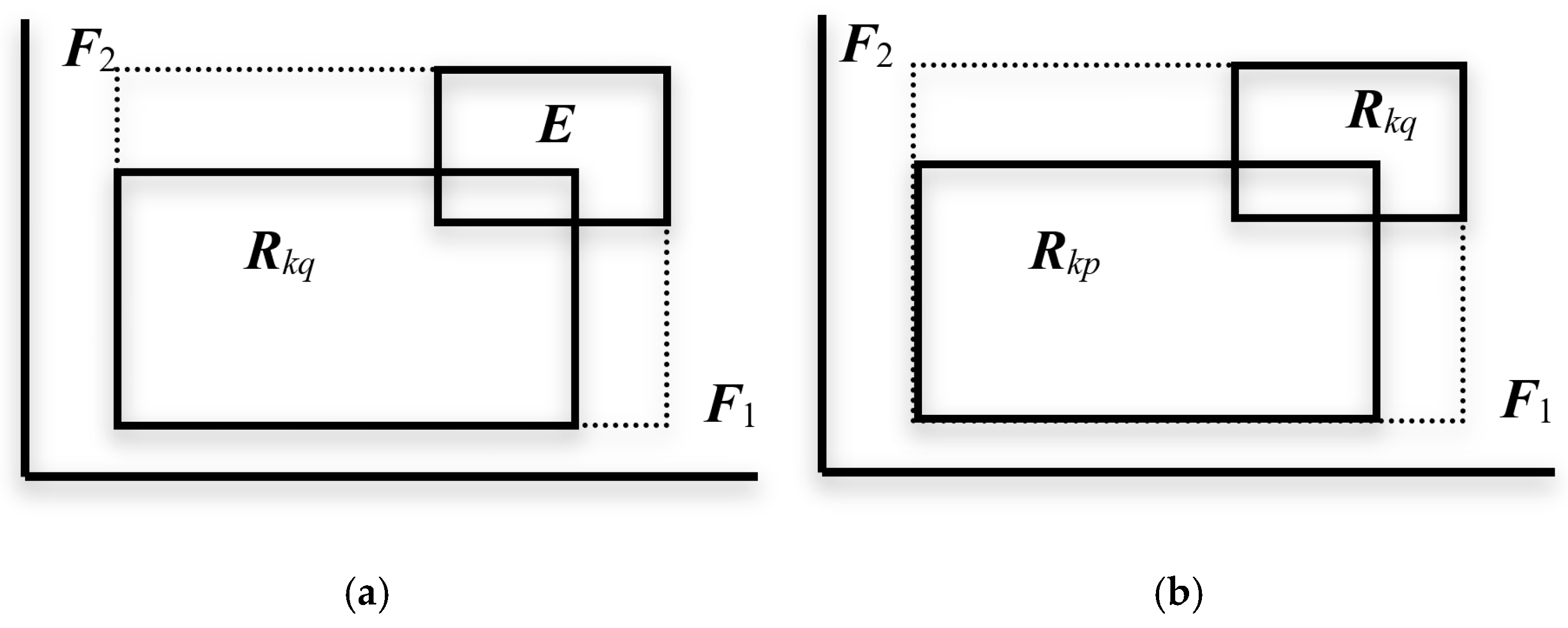
If the description E in Figure 5a is completely included in the region Rkq, Property (3) becomes valid. Figure 5b illustrates Property (4).

2.3.2. Classification Rule

Let a given pattern ω be described by E in the feature space D(d). The given pattern ω is determined to come from class Ck if there exists a sub-concept Ωkq for which the similarity S(ωΩkq) is the largest.
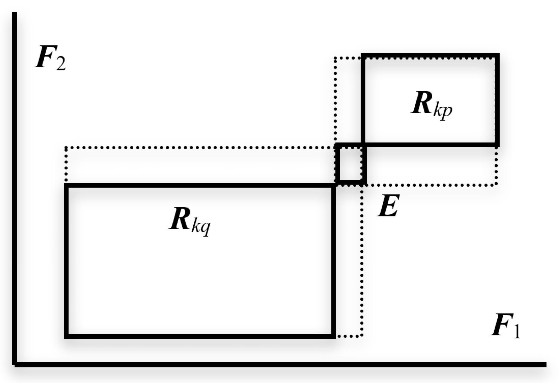
It is clear that our basic problem is how to generate a sufficiently small number of subclasses that satisfy conditions (17) and (18) for each pattern class. However, it should be noted that, from Property (4) of our similarity measure, a description R with a larger object size in the feature space asserts a greater similarity to the description E of the given pattern ω (see Figure 6), while the “generality” of sub-concept Ω (i.e., the “number of sample patterns” included in Ω) corresponding to R is not directly related to the concept size of R. From this reason, we use the “compactness” to evaluate the description of a subclass in the feature space. We also use the “mutual neighborhood concept” [7] in order to assure the separability between pattern classes.

2.3.3. Generation of Subclasses by the Supervised Hierarchical Conceptual Clustering

Sample patterns ωkp, ωkqUk of pattern class Ck are called mutual neighbors [7] against other classes Cj, j = 1, 2, …, M (jk), if any sample ωjrUj, r = 1, 2, …, Nj; j = 1, 2, …, M (jk), is separated from the Cartesian join of ωkp and ωkq:
(EkpEkq)⊠Ejr = , r =1, 2, …, Nj; j = 1, 2, …, M, (j ≠ k).
For each pattern class Ck, let Cck denote all other pattern classes except Ck, and let Uck be the union of the training sets Uj, j = 1, 2, , M (jk). Then, the subclass generation based on the supervised hierarchical conceptual clustering (SHCC) is summarized as follows.
Algorithm SHCC for generating subclasses (for pattern class Ck):
We assume that each Nk sample pattern in Uk is itself a subclass of Ck.
Step (1)
For each pair of subclasses ω and ω’ in Uk, calculate the compactness C(ω, ω’) = P(EE) and find the pair ωp and ωq in Uk that minimizes C(ωp, ωq) = P(EpEq) and satisfies also the mutual neighborhood condition in (20) against Uck.
Step (2)
Define the new subclass ωpq by the set {ωp, ωq}. Then, delete ωp and ωq from Uk and put the new subclass ωpq into Uk, where the subclass ωpq is described by the Cartesian join Epq = EpEq in the feature space D(d).
Step (3)
Repeat Step (1) and Step (2) until the set Uk is unchanged.
Step (4)
Define the subclasses Ωk1, Ωk2, …, Ωkm and their descriptions Rk1, Rk2, …, Rkm in the feature space from the generated subclasses in Uk according to the cardinality of the subclasses from the largest to the smallest. (End of algorithm)
Using this algorithm, we can reduce the given set of Nk sample patterns to m subclasses. It should be noted that there is a possibility that some original sample patterns remain as subclasses depending on the interclass structure between Ck and Cck (see Figure 4).

3. Experimental Results

3.1. Artificial Data

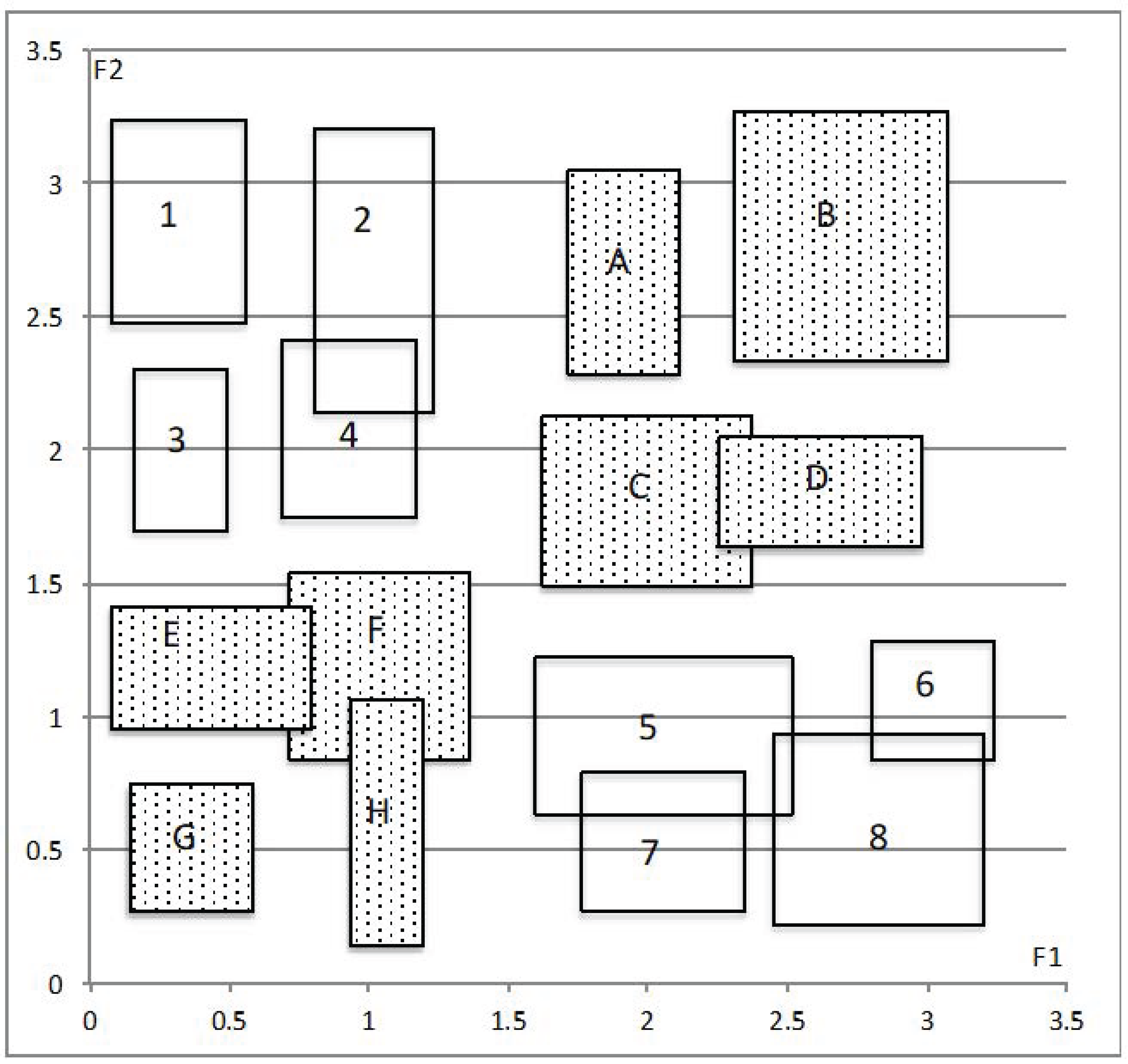
In this data, two pattern classes have two subclasses, respectively, and they follow the X-or form in the plane by F1 and F2, as shown in Figure 7. We use the zero one normalized data in Table 3 to describe the clustering steps. In this table, F3, F4, and F5 are randomly generated useless features; class C1 is composed of samples numbered from 1 to 8, and the other class C2 is composed of samples A to H.
Table 4 and Table 5 summarize clustering steps to generate subclasses for each pattern class. In Table 4, the compactness of subclass (7, 8), for example, is calculated as follows:
C(7, 8) = ((0.985 − 0.530) + (0.254 − 0.030) + (0.564 − 0.221) + (0.666 − 0.259) + (0.600 − 0.319))/5 = 0.342.
Table 4. Subclass generation for class C1 by the SHCC.
StepsSubclassC(p, q)F1F2F3F4F5
1(7, 8)0.420E, F, G, HA, B, C, DFC, EC, E, F
2(1, 3)0.446A, B, C, DE, F, G, H C, D, GB, E, F
3(2, 4)0.547A, B, C, DE, F, G, H EF
4((7, 8), 6)0.580E, F, G, HA, B, C, D EF
5((1, 3), (2, 4))0.668A, B, C, DE, F, G, H
6(((7, 8), 6), 5)0.694E, F, G, HA, B, C, D F
C11(1, 2, 3, 4)0.429[0.000, 0.379][0.507, 0.985]
C12(5, 6, 7, 8)0.429[0.485, 1.000][0.030, 0.373]
Table 5. Subclass generation for class C2 by the SHCC.
StepsSubclassC(p, q)F1F2F3F4F5
1(A, C)0.3871, 2, 3, 45, 6, 7, 8618
2(G, H)0.4145, 6, 7, 81, 2, 3, 44, 61, 6
3((A, C), D)0.5381, 2, 3, 45, 6, 7, 84, 61
4((G, H), F)0.5665, 6, 7, 81, 2, 3, 461
5(((G, H), F), E)0.6285, 6, 7, 81, 2, 3, 46
6(((A, C), D), B)0.6611, 2, 3, 45, 6, 7, 861
C21(E, F, G, H)0.628[0.000, 0.394][0.000, 0.448]
C22(A, B, C, D)0.661[0.485, 0.955][0.433, 1.000]
These tables summarize how each feature separates samples from the opposite class. As the results, we could have subclass pairs (C11, C12) and (C21, C22) that compose X-or structure in the plane by the selected features, F1 and F2.

3.2. The Hardwood Data

The data is selected from the US Geological Survey (Climate—Vegetation Atlas of North America) [8]. The following eight features describe ten selected hardwoods:
F1: Annual temperature (ANNT) (°C);
F2: January temperature (JANT) (°C);
F3: July temperature (JULT) (°C);
F4: Annual precipitation (ANNP) (mm);
F5: January precipitation (JANP) (mm);
F6: July precipitation (JULP) (mm);
F7: Growing degree days on 5 °C base ×1000 (GDC5);
F8: Moisture index (MITM).
Table 6 shows the min-max descriptions for the selected ten hardwoods data. The original data is quantile representation by seven quantile values for 0, 10, 25, 50, 75, 90, and 100 (%). We select here only 0% and 100% quantile values, since these values describe well the differences between clusters in the unsupervised hierarchical conceptual clustering [5]. In this example, class C1 and class C2 are composed of east hardwoods {E1, E2, E3, E4, E5} and west hardwoods {W1, W2, W3, W4, W5}, respectively.
Table 7 and Table 8 summarize the clustering steps to generate subclasses to each class by the SHCC. From Table 7, east hardwoods are reduced to the class C1 = (E1, E2, E3, E4, E5) and separated from west hardwoods with respect to F1max, F4max, F5min, and F6min.
On the other hand, west hardwoods are separated into subclasses C21 = (W1, W2, W3) and C22 = (W1, W2). Subclass C21 is separated from class C1 with respect to F1max, F2min, F5min, F6min, F8min, and F8max, while C22 is separated from class C1 with respect to F1max, F2max, F4min, F4max, F5min, F5max, F6min, and F7max.
Since F6min has null concept size for C21 and C22, we use the representation in Table 9 for each class.
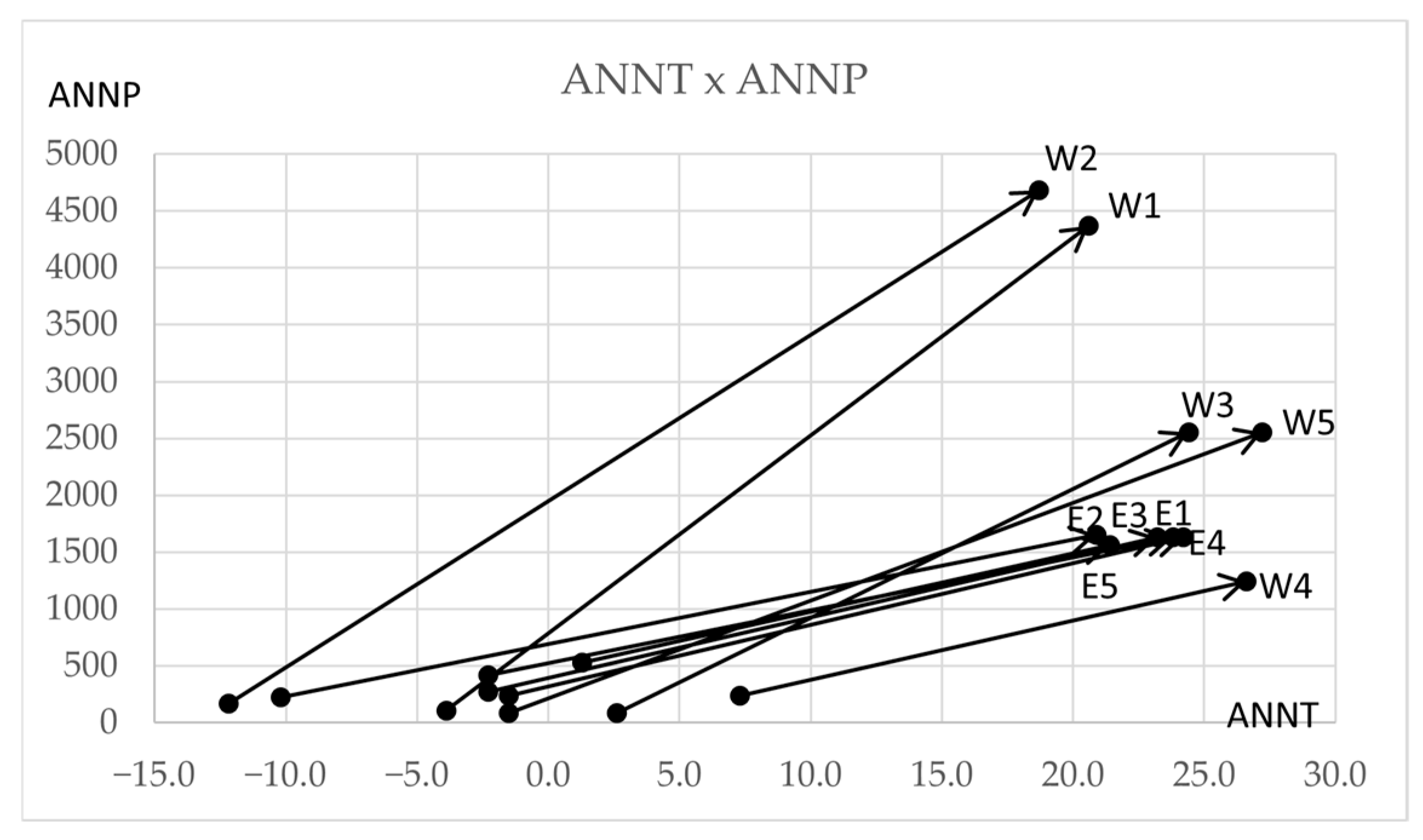
Figure 8 shows the scatter diagram of the given hardwoods. In this figure, the maximum vertices of the west hardwoods of C21 surround the maximum vertices of the east hardwoods.
Table 10 contains test data to check the property of our classification model. Table 11 summarizes the similarity of each test sample to the subclasses. BETURA is classified as C22 with the similarity value one. CARYA and TILIA are classified as C21 and C1, respectively, with high similarity values. Both CASTANEA and ULMUS are classified to class C1 with slightly degraded similarity values compared to CARYA and TILIA. Figure 9 summarizes mutual positions of test samples and the ten hardwoods initially given. This figure shows that there is a difficulty in distinguishing between class C1 and subclass C21.

3.3. Golf Data [9]

The Golf data in Table 12 is described by four features having the following possible values or ranges:
F1: Outlook = {overcast, rain, sunny}, F2: Temperature = [64, 85],
F3: Humidity = [65, 96], and F4: Windy = {TRUE, FALSE}.
Therefore, from (9), we have
|D1| = 3, |D2| = 85 − 64 = 21, |D3| = 96 − 65 = 31, and |D4| = 2.
The compactness (15) of samples 1 and 2 in class C1, for example, is calculated as follows:
C(1, 2) = {1/3 + (83 − 72)/21 + (90 − 78)/31 + 2/2}/4 = 0.561.
Table 12. Golf data.
ClassSampleF1: OutlookF2: Temp. (℉)F3: Humidity (%)F4: Windy
1Overcast7290TRUE
2Overcast8378FALSE
3Rainy7580FALSE
4Overcast6465TRUE
C15Sunny7570TRUE
(Play)6Overcast8175FALSE
7Rainy6880FALSE
8Rainy7096FALSE
9Sunny6970FALSE
ARainy7180TRUE
BRainy6570TRUE
C2CSunny8090TRUE
(Don’t play)DSunny8585FALSE
ESunny7295FALSE
In this example, class C1 and class C2 are composed of the set {1, 2, 3, 4, 5, 6, 7, 8, 9} and the set {A, B, C, D, E}, respectively. Table 13 summarizes the result of the SHCC for class C1 (play). We have three subclasses: C11 = (1, 2, 4, 6), C12 = (3, 7, 8), and C13 = (5, 9). Subclass C11 is described by the single feature value “Outlook = Overcast”, and the compactness is 0.333. Subclass C12 is described as “Outlook = Rainy and Windy = FALSE”, and the compactness is 0.417. Subclass C13 is described as “Outlook = Sunny and Humidity = 70”, and the compactness is 0.167.
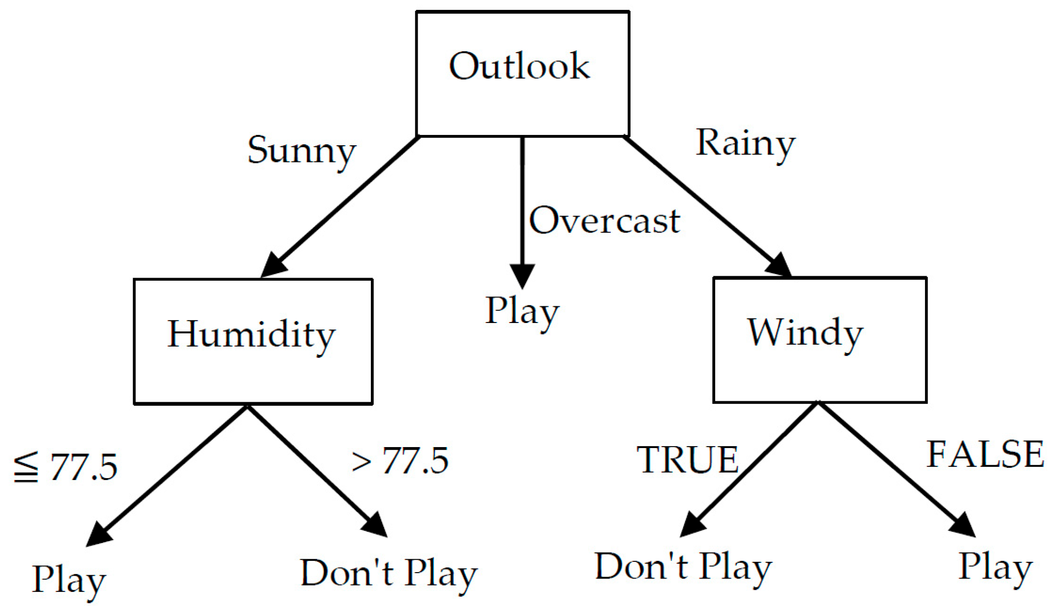
On the other hand, from Table 14, we have C21 = (C, D, E) and C22 = (A, B) with the compactness 0.328 and 0.417, respectively. Subclass C21 is described as “Outlook is Sunny and Humidity = [85, 95]”, and C22 as “Outlook = Rainy and Windy = TRUE”. These class descriptions are easily summarized as the decision tree in Figure 10, where Humidity = 77.5 is the midpoint value between [70, 70] and [85, 95].

4. Discussion

This paper presented a region-oriented pattern classification method for mixed feature-type data based on the Cartesian system model (D(d), ⊞, ⊠). We defined the notion of the concept size and then the compactness for objects and/or clusters in the feature space D(d) as the measure of similarity based on the Cartesian join operator ⊞. In unsupervised hierarchical conceptual clustering, the compactness played not only the role of the similarity measure, but also as the roles of the cluster quality measure and the feature-effectiveness criterion. By minimizing the compactness in each clustering step, we could find the meaningful structures, e.g., a functional structure and a cluster structure with respect to the obtained robustly informative features.
On the other hand, in the supervised hierarchical conceptual clustering of a given pattern class, we used the mutual neighborhood condition based on the Cartesian meet ⊠ to assure the separability of the class from other pattern classes, in addition to the evaluation of the compactness in each clustering step.
In the X-or problem, two pattern classes are mutually overlapped in each of the given five features. By the supervised hierarchical conceptual clustering, two subclasses of each pattern class organizing X-or form are exactly detected with respect to the selected first two features.
In the hardwood data, the SHCC generated a single class description C1 for the east hardwoods and two subclasses C21 and C22 for the west hardwoods. For the selected informative features, the scatter diagram and the classification results of test samples show a difficulty for clear separation between class C1 and subclass C21.
In the golf data, the SHCC generated three subclasses, C11 = {Outlook = Overcast}, C12 = {Outlook = Rainy and Windy = FALSE}, and C13 = {Outlook = Sunny and Humidity =70} for class C1 = (Play), while two subclasses, C21 = {Outlook = Sunny and Humidity = [85, 95]} and C22 = {Outlook = Rainy and Windy =TRUE}, for class C2 = (Don’t play) without any feature evaluation criterion used in, for example, ID3/C4.5. These results easily lead to the decision tree in Figure 10.
Finally, we should note that we could obtain subclass descriptions with informative features by applying the supervised hierarchical conceptual clustering to each pattern class against other pattern classes. This approach largely simplifies the process to design a pattern classifier for mixed feature-type symbolic data.

Author Contributions

Conceptualization and methodology, M.I. and H.Y.; original draft preparation, M.I. All authors have read and agreed to the published version of the manuscript.

Funding

This work was supported by JSPS KAKENHI (Grants-in-Aid for Scientific Research) Grant Number 25330268.

Conflicts of Interest

The authors declare no conflicts of interest.

References

  1. Liu, H.; Motoda, H. Computational Methods of Feature Selection; CRC Press: London, UK, 2007. [Google Scholar]
  2. Miao, J.; Niu, L. A survey on feature selection. Procedia Comput. Sci. 2016, 91, 919–926. [Google Scholar] [CrossRef]
  3. Solorio-Fernández, S.; Martínez-Trinidad, J.F.; Carrasco-Ochoa, J.A. A review of unsupervised feature selection methods. Artif. Intell. Rev. 2020, 53, 907–948. [Google Scholar] [CrossRef]
  4. Billard, L.; Diday, E. Symbolic Data Analysis: Conceptual Statistics and Data Mining; Wiley: Chichester, UK, 2007. [Google Scholar]
  5. Huang, H.S. Supervised feature selection: A tutorial. Artif. Intell. Res. 2015, 4, 22–37. [Google Scholar] [CrossRef]
  6. Ichino, M.; Umbleja, K.; Yaguchi, H. Unsupervised feature selection for histogram-valued symbolic data using hierarchical conceptual clustering. Stats 2021, 4, 359–384. [Google Scholar] [CrossRef]
  7. Ichino, M.; Yaguchi, H. Symbolic pattern classifiers based on the Cartesian system model. In Data Science, Classification, and Related Methods; Hayashi, C., Yajima, K., Bock, H.-H., Ohsumi, N., Tanaka, Y., Baba, Y., Eds.; Springer: Berlin/Heidelberg, Germany, 1998. [Google Scholar]
  8. Histogram Data by the U.S. Geological Survey, Climate-Vegetation Atlas of North America. Available online: http://pubs.usgs.gov/pp/p1650-b/ (accessed on 20 November 2010).
  9. Wu, X.; Kumar, V. (Eds.) The Top Ten Algorithms in Data Mining; Chapman and Hall/CRC: New York, NY, USA, 2009. [Google Scholar]
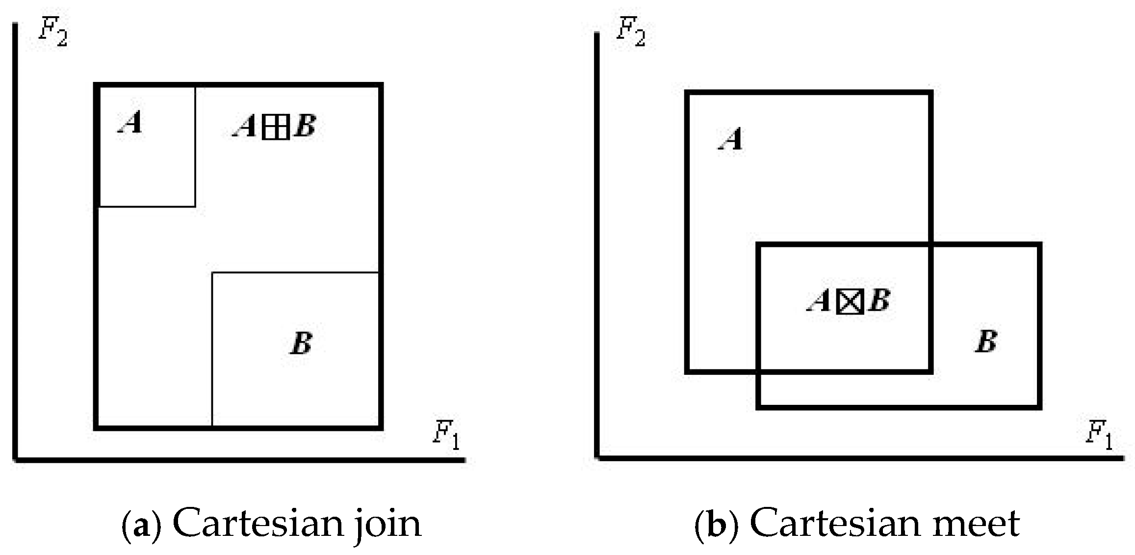
Figure 1. The Cartesian join and the Cartesian meet in the Euclidean plane.
Stats 08 00076 g001
Figure 2. A counter example of property (6).
Stats 08 00076 g002
Figure 3. The results of the fats and oils data for iodine value (I) and specific gravity (S).
Stats 08 00076 g003
Figure 4. Illustration for condition (16).
Stats 08 00076 g004
Figure 5. Illustrations for the properties of the asymmetric similarity measure.
Stats 08 00076 g005
Figure 6. Illustration for the relation S(ωΩkp) ≤ S(ωΩkq).
Stats 08 00076 g006
Figure 7. A two-dimensional X-or problem.
Stats 08 00076 g007
Figure 8. The scatter diagram of the hardwood data.
Stats 08 00076 g008
Figure 9. The Scatter diagram of the test data.
Stats 08 00076 g009
Figure 10. Decision tree for the golf data.
Stats 08 00076 g010
Table 2. Descriptions of two pattern classes for the fats and oils data.
ClassF1F2F3F4F5
Plant oils[0.914, 0.937][−27, 6][79, 208][118, 198][0.42, 4.85]
Fats[0.858, 0.870][22, 38][40, 77][190, 202][0.31, 3.65]
Table 3. The X-or data.
SampleF1 MinF1 MaxF2 MinF2 MaxF3 MinF3 MaxF4 MinF4 MaxF5 MinF5 Max
10.0000.1820.7460.9850.3860.5900.0000.1500.3670.992
20.2120.3790.6570.9700.2990.3300.2621.0000.5070.524
30.0450.1210.5070.6870.4680.9060.1120.4260.5850.776
40.1970.3640.5220.7310.7780.9490.4090.8560.1570.877
50.4850.7730.1490.3580.0001.0000.0200.8000.7140.781
60.8481.0000.2240.3730.9250.9410.7220.8930.0440.778
70.5300.6970.0450.2090.2210.4100.3420.6660.3630.600
80.7270.9850.0300.2540.4590.5640.2590.6090.3190.338
A0.5150.6520.6720.9400.3010.4850.3350.4800.5220.984
B0.6970.9550.7011.0000.1080.8620.2970.7670.2350.339
C0.4850.7120.4330.6420.2270.5110.6730.8580.6850.944
D0.6820.9090.4780.6120.3990.4480.4660.4890.0300.725
E0.0000.2270.2390.4180.3100.8770.1120.1510.0000.179
F0.2120.3940.2240.4480.6680.7990.3030.7520.9711.000
G0.0300.1670.0600.1550.2830.4060.5160.5370.4790.848
H0.2580.3640.0000.2990.2110.6290.3520.3860.0130.735
Table 6. The hardwoods data [8].
Taxon NameANNT: F1JANT: F2JULT: F3ANNP: F4JANP: F5JULP: F6GDC5: F7MITM: F8
ACER EAST: E1 min −2.3−24.611.541510560.50.62
max23.818.928.816301662226.81.00
ACER WEST: W1 min−3.9−23.87.1105500.10.14
max20.611.029.243706161605.61.00
ALNUS EAST: E2 min−10.2−30.97.12209280.10.22
max20.914.129.116501662125.91.00
ALNUS WEST: W2 min−12.2−30.57.1170400.10.22
max18.710.828.346856674524.81.00
FRAXINUS EAST: E3 min−2.3−23.813.52706180.80.39
max23.218.129.516301662186.71.00
FRAXINUS EAST: W3 min2.6−7.412.585500.90.09
max24.416.933.125554142066.90.97
JUGLANS EAST: E4 min1.3−14.615.25259411.00.63
max21.412.429.415601502046.01.00
JUGLANS WEST: W4 min7.3−1.317.1235101.60.20
max26.626.231.312451663288.50.94
QUERCUS EAST: E5 min−1.5−22.713.52407320.80.21
max24.219.631.816301612227.01.00
QUERCUS EAST: W5 min−1.5−12.09.785100.30.08
max27.226.233.825554003508.50.99
Table 7. Subclass generation for east hardwoods by the SHCC.
Steps1 2 3 4
Subclass(E1, E4) ((E1, E4), E3) (((E1, E4),
E3), E5)
((((E1, E4), E3), E5), E2)
C(p, q) = 0.520SeparabilityC(p, q) = 0.562SeparabilityC(p, q) = 0.604SeparabilityC(p, q) = 0.671Separability
F1min[−2.3, 1.3]W1–W4[−2.3, 1.3]W1–W4[−2.3, 1.3]W1–W4[−10.2, 1.3]W2, W3, W4
F1max[21.4, 23.8]W1–W5[21.4, 23.8]W1–W5[21.4, 24.2]W1–W5[20.9, 24.2]W1–W5
F2min[−24.6, −14.6]W2, W3, W4, W5[−24.6, −14.6]W2, W3, W4, W5[−24.6, −14.6]W2, W3, W4, W5[−30.9, −14.6]W3, W4, W5
F2max[12.4, 18.9]W1, W2, W4, W5[12.4, 18.9]W1, W2, W4, W5[12.4, 19.6]W1, W2, W4, W5[12.4, 19.6]W1, W2, W4, W5
F3min[11.5, 15.2]W1, W2, W4, W5[11.5, 15.2]W1, W2, W4, W5[11.5, 15.2]W1, W2, W4, W5[7.1, 15.2]W4
F3max[28.8, 29.4]W2–W5[28.8, 29.5]W2–W5[28.8, 31.8]W2, W3, W5[28.8, 31.8]W2, W3, W5
F4min[415, 525]W1–W5[270, 525]W1–W5[240, 525]W1–W5[220, 525]W1, W2, W3, W5
F4max[1560, 1630]W1–W5[1560, 1630]W1–W5[1560, 1630]W1–W5[1560, 1650]W1–W5
F5min[9, 10]W1–W5[6, 10]W1–W5[6, 10]W1–W5[6, 10]W1–W5
F5max[150, 166]W1, W2, W3, W5[150, 166]W1, W2, W3, W5[150, 166]W1, W2, W3, W5[150, 166]W1, W2, W3, W5
F6min[41, 56]W1–W5[18, 56]W1–W5[18, 56]W1–W5[18, 56]W1–W5
F6max[204, 222]W1, W2, W4, W5[204, 222]W1, W2, W4, W5[204, 222]W1, W2, W4, W5[204, 222]W1, W2, W4, W5
F7min[0.5, 1.0]W1, W2, W4, W5[0.5, 1.0]W1, W2, W4, W5[0.5, 1.0]W1, W2, W4, W5[0.1, 1.0]W4
F7max[6.0, 6.8]W1–W5[6.0, 6.8]W1–W5[6.0, 7.0]W1, W2, W4, W5[5.9, 7.0]W1, W2, W4, W5
F8min[0.62, 0.63]W1–W5[0.39, 0.63]W1–W5[0.21, 0.63]W1, W3, W4, W5[0.21, 0.63]W1, W3, W4, W5
F8max[1.0, 1.0]W3, W4, W5[1.0, 1.0]W3, W4, W5[1.0, 1.0]W3, W4, W5[1.0, 1.0]W3, W4, W5
Table 8. Subclass generation for west hardwoods by the SHCC.
Steps1 2 3
Subclass(W3, W4) ((W3, W4), W5) (W1, W2)
C(p, q) = 0.714SeparabilityC(p, q) = 0.775SeparabilityC(p, q) = 0.872Separability
F1min[2.6, 7.3]E1–E5[−1.5, 7.3]E1, E2, E3[−12.2, −3.9]E1, E3, E4
F1max[24.4, 26.6]E1–E5[24.4, 27.2]E1–E5[18.7, 20.6]E1–E5
F2min[−7.4, −1.3]E1–E5[−12.0, −1.3]E1–E5[−30.5, −23.8]E2, E4, E5
F2max[16.9, 26.2]E2, E4[16.9, 26.2]E2, E4[10.8, 11.0]E1–E5
F3min[12.5, 17.1]E1, E2[9.7, 17.1]E2[7.1, 7.1]E1, E3, E4, E5
F3max[31.3, 33.1]E1, E2, E3, E4[31.3, 33.8]E1, E2, E3, E4[28.3, 29.2]E3, E4, E5
F4min[85, 235]E1, E3, E4, E5[85, 235]E1, E3, E4, E5[105, 170]E1–E5
F4max[1245, 2555]None[1245, 2555]None[4370, 4685]E1–E5
F5min[1, 5]E1–E5[1, 5]E1–E5[4, 5]E1–E5
F5max[166, 414]E4, E5[166, 414]E4, E5[616, 667]E1–E5
F6min[0, 0]E1–E5[0, 0]E1–E5[0, 0]E1–E5
F6max[206, 328]E4[206, 350]E4[160, 452]None
F7min[0.9, 1.6]E1, E2, E3, E5[0.3, 1.6]E2[0.1, 0.1]E1, E3, E4, E5
F7max[6.9, 8.5]E1, E2, E3, E4[6.9, 8.5]E1, E2, E3, E4[4.8, 5.6]E1–E5
F8min[0.09, 0.20]E1–E5[0.08, 0.20]E1–E5[0.14, 0,22]E1, E3, E4
F8max[0.94, 0.97]E1–E5[0.94, 0.99]E1–E5[1.0, 1.0]None
Table 9. Three subclasses obtained for the hardwood data.
ClassANNT MaxANNP MaxJANP Min
C1: E1–E5[20.9, 24.2][1560, 1650][6, 10]
C21: W3, W4, W5[24.2, 27.2][1245, 2555][1, 5]
C22: W1, W2[18.7, 20.6][4370, 4685][4, 5]
Table 10. A test dataset.
Taxon NameANNTANNPJANP
BETURA[−13.4, 20.3][90, 4370][4, 612]
CARYA[3.6, 23.5][410, 1755][2, 150]
CASTANEA[4.4, 21.5][765, 1630][32, 150]
TILIA[1.1, 19.9][415, 1560][9, 150]
ULMUS[−2.3, 23.8][325, 1145][6, 166]
Table 11. The similarity values of the test hardwoods to each pattern class.
ClassFeaturesBETURACARYACASTANEATILIAULMUS
C1F1max0.846110.7671
F4max0.0320.462110.178
F5min0.6670.50.15411
Avg.0.5040.6540.7180.9220.726
C21F1max0.0740.8110.5260.4110.235
F4max0.4191110.929
F5min110.1290.50.8
Avg.0.4980.9370.5520.6370.655
C22F1max10.3960.67910.373
F4max10.1080.1030.1010.089
F5min110.0360.20.8
Avg.10.5010.2720.4030.421
Table 13. Subclass generation for class C1 (Play) by the SHCC.
StepsSubclassC(p, q)OutlookTemp.HumidityWindy
1(2, 6)0.256A, B, C, D, EA, B, C, D, EA, B, C, D, EA, B, C
2(3, 7)0.291C, D, EB, C, DB, C, D, EA, B, C
3(5, 9)0.405A, BB, C, EA, C, D, EA, B, C
4((3, 7), 8)0.421C, D, EC, DB, DA, B, C
5(1, 4)0.505A, B, C, D, EC, DED, E
6((2, 6), (1, 4))0.761A, B, C, D, EDE
C11(1, 2, 4, 6)0.333Overcast
C12(3, 7, 8)0.417Rainy FALSE
C13(5, 9)0.167Sunny [70, 70]
Table 14. Subclass generation for class C2 (Don’t play) by the SHCC.
StepsSubclassC(p, q)OutlookTemp.HumidityWindy?
1(C, D)0.2441, 2, 3, 4, 6, 7, 81, 3, 4, 5, 7, 8, 92, 3, 4, 5, 6, 7, 8, 9
2(A, B)0.3601, 2, 4, 5, 6, 97, 8, 92, 3, 5, 6, 7, 92, 3, 6, 7, 8, 9
3((C, D), E)0.5691, 2, 3, 4, 6, 7, 81, 2, 3, 5, 62, 3, 4, 5, 6, 7, 8, 9
C21(C, D, E)0.328Sunny [85, 95]
C22(A, B)0.417Rainy TRUE
Disclaimer/Publisher’s Note: The statements, opinions and data contained in all publications are solely those of the individual author(s) and contributor(s) and not of MDPI and/or the editor(s). MDPI and/or the editor(s) disclaim responsibility for any injury to people or property resulting from any ideas, methods, instructions or products referred to in the content.