Abstract
An ordered heterogeneity (OH) test is a test for a trend that combines a nondirectional heterogeneity test with the rank-order information specified under the alternative. A modified OH test introduced in 2006 can detect all possible patterns under the alternative with a relatively high power. Here, it is proposed to apply the modified OH test as a permutation test, which has the advantage that it requires only the exchangeability of the observations in the combined sample under the null hypothesis. No additional assumptions or simulations of critical values are necessary. A simulation study indicates that the permutation OH test controls the significance level even for small sample sizes and has a good power, comparable to competing tests. Moreover, the main advantage of the OH tests is their very broad applicability; they can always be applied when a heterogeneity test exists.
1. Introduction
Studies that compare more than two groups are widespread. In clinical dose-finding trials and other studies such as agricultural experiments, often increasing doses of the same drug or fertilizer are investigated. In these cases, there is an intrinsic order in the treatments. Usually only a few doses are studied, for instance, a placebo group and two or three doses. Then it is suitable and common to treat the dose level as a discrete variable [1]. Moreover, one might assume that an effect does not decline with increasing dose levels. Then, an appropriate alternative hypothesis is a trend: an increase in the effect with an increase in the dose level. In this case, the alternative is ordered, and a so-called trend test can be applied. Trend tests are particularly sensitive for detecting an ordered alternative.
For illustration, we consider a one-way design with k independent groups, appropriate, for example, in randomized parallel dose–response trials. The sample size of group i, i = 1, …, k, is denoted by , and let be the i-th random sample distributed according to a distribution function . Observations within samples are assumed to be independent and identically distributed, and mutual independence between samples is assumed. In the location-shift model, there is no difference under the null hypothesis
where is the location parameter associated with group i. We assume that the (i = 1, …, k) do not decline with increasing dose levels; therefore, trend tests are considered, and the null hypothesis is tested against the ordered alternative
Rice and Gaines [2,3] introduced the ordered-heterogeneity family of tests. The idea is to combine the p-value from a nondirectional heterogeneity test with the independent rank-order information specified under the alternative. The test statistic proposed by Rice and Gaines [2,3] is , where is the p-value of a heterogeneity test and is Spearman’s rank correlation. Note that Spearman’s rank correlation is Pearson’s product-moment correlation coefficient computed based on ranks [4]. Rice and Gaines [3] presented critical values for the ordered heterogeneity (OH) test determined under the assumptions that is uniform on (0, 1) and independent of .
Rice and Gaines [2,3] pointed out that the OH test has a wide range of both parametric and nonparametric applications. They did not claim that the OH test has the highest power, but the advantage is its simplicity and broad applicability. The principle “permits one to easily convert almost any nondirectional heterogeneity test into a directional test” [2]. In the example discussed by Rice and Gaines [2], there are three populations of fruit flies with increasing variances under the alternative.
Neuhäuser and Hothorn [5] introduced modifications of the ordered heterogeneity test that are more robust. On the one hand, under the assumption , there are 2k−1 different orderings. When we consider k = 3 as an example, there are the orderings , , and in addition to the null hypothesis . The corresponding expected ranks (using mid-ranks for ties) of the non-null scenarios are (1, 2, 3), (1.5, 1.5, 3), and (1, 2.5, 2.5). For all the 2k−1 − 1 scenarios under the trend alternative, Spearman’s rank correlation can be computed, and the maximum can be multiplied with . Moreover, the observed ordering of the groups can be obtained not only using sample means but also using the mean ranks of the groups.
The usefulness of mean ranks was illustrated by Neuhäuser and Hothorn [5] with an example. The dry weight of spinach was investigated for five different doses. The smallest value was observed in the group with the second largest dose. Due to this outlier, the ranking of the sample means is (2, 4, 3, 1, 5). However, the ranking of the mean ranks is (1, 2, 4, 3, 5), which leads to a much larger correlation and test statistic.
Through the use of mean ranks and/or the maximum correlation, Neuhäuser and Hothorn [5] considered the following four different OH tests:
- OH1: ordering of the groups according to the sample means and test based on the expected ranks (1, 2, …, k);
- OH2: ordering of the groups according to the mean ranks and test based on the expected ranks (1, 2, …, k);
- OH3: ordering of the groups according to the sample means and test based on the maximum rank correlation out of the 2k−1 − 1 possible expected ranks;
- OH4: ordering of the groups according to the mean ranks and test based on the maximum rank correlation out of the 2k−1 − 1 possible expected ranks.
In the simulations presented by Neuhäuser and Hothorn [5], the OH4 test showed the best results with relatively high power for all possible patterns under the trend alternative, as well as for normal and non-normal distributions.
The critical values given by Rice and Gaines [3] cannot be utilized for the tests using the maximum rank correlation. Therefore, Neuhäuser and Hothorn [5] simulated critical values. To be precise, was generated from a uniform distribution on (0, 1), and correlations were obtained as rank correlations between independent samples of size k taken from simulated standard normal distributions. However, both the assumptions needed by Rice and Gaines [3] for their numerical calculation of critical values and the simulations performed by Neuhäuser and Hothorn [5] are no longer needed because, nowadays, permutation tests can easily be carried out with the test statistics and , respectively. In a permutation test, inference is based on the permutation null distribution of the test statistic, which can be generated by considering all possible permutations under the null hypothesis; that is, the test statistic is computed for each permuted data set to obtain the null distribution. A p-value can be obtained from this null distribution as the proportion of permutations with an equal or more extreme value of the test statistic than the actually observed value of the test statistic [6]. In the considered one-way design, each permutation is a possible reallocation of the observed values to k groups of sizes . Often, a permutation test is preferable to traditional tests because of its exactness [7].
The number of possible permutations can be very large, especially for large values of k. However, in an approximate permutation test, the permutation distribution can be estimated based on a simple random sample of, e.g., B = 1000 permutations. According to Bonnini et al. [6], this number of 1000 permutations is sufficient; it gives a good degree of approximation and therefore reliable results. Marozzi [8] suggested 500 to 1000 permutations when estimating the size and power of a permutation test at level α = 0.05 in simulation studies. However, for smaller significance levels and for actual applications, more permutations should be used [8].
2. Materials and Methods
In this paper, we investigate (approximate) OH permutation tests based on and and compare these tests with two competing trend tests. On the one hand, we consider the test proposed by Jonckheere [9], which is a nonparametric trend test based on Mann–Whitney scores. This test usually is considered the standard non-parametric trend test for the one-way design [4]. On the other hand, we include the test of Shan et al. [10] that can be considered as an extension of Jonckheere’s test and additionally includes the rank difference between observations from different groups. There are further trend tests, as, e.g., a nonparametric test proposed by Cuzick [11], which is based on rank sums. This test was included in the simulation study presented by Shan et al. [10] and was considered not preferable to their proposed trend test [10].
A Monte Carlo simulation study was performed using R (version 4.4.1); 10,000 simulation runs were generated for each configuration, and approximate permutation tests were carried out based on B = 1000 permutations. The Kruskal–Wallis test was used as the heterogeneity test to obtain . The trend tests of Jonckheere [9] and Shan et al. [10] were also performed as approximate permutation tests.
3. Results
3.1. Simulation Study
Here we present results for sample sizes = 10 (see Table 1, Table 2 and Table 3) and = 20 (see Figure 1). Even for the small sample size = 10, the actual type I error rate (size) is close to the nominal significance level. Although permutation tests guarantee the significance level α, there are simulated actual type I error rates slightly larger than the chosen α of 5% due to the error margin of the simulation. However, the approximate OH permutation trend tests, as well as the competing tests, have good and similar type I error rates.

Table 1.
Simulated size and power of different permutation trend tests for the location-shift model , where is distributed as specified (k = 3, = 10, α = 0.05).
Table 2.
Simulated size and power of different permutation trend tests for the location-shift model , where is distributed as specified (k = 4, = 10, α = 0.05).
Table 3.
Simulated size and power of different permutation trend tests for the location-shift model , where is distributed as specified (k = 5, = 10, α = 0.05).
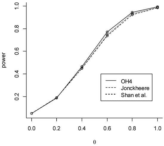
Figure 1.
Simulated size and power of different permutation trend tests for the location-shift model with means 0, 0, , and , where the data are normally distributed with variance 1 (k = 4, = 20, α = 0.05).
In Table 1, Table 2 and Table 3, the test with the largest power is highlighted in bold for each scenario. We can confirm that OH4 is the best of the four OH permutation trend tests. This test has a good power, which is comparable to that of the standard trend tests of Jonckheere or Shan et al. Although in several considered scenarios the test proposed by Shan et al. [10] has the highest power, there are also scenarios where OH4 has the highest power (see, e.g., Figure 1). As expected, because no single trend test is uniformly most powerful [3], the simulation study does not show a clear winner. The tests OH4 and Jonckheere do not differ much.
3.2. Example
Raw data of reaction times (in seconds) of mice in a control group and three further groups with increasing doses were presented by Shirley [12]. The sample size is ten per group. Since the distribution of the reaction time is highly skewed [12], non-parametric methods seem preferable. With the data from all four groups, trend tests give a clear significance with, e.g., p < 0.0001 in the Jonckheere test. Therefore, hereafter, the control group is omitted for illustrative purposes. With the remaining three groups, permutation tests were performed with B = 100,000 permutations.
Although the Kruskal–Wallis test is not significant with a p-value larger than 10%, the OH tests that combine the Kruskal–Wallis test with Spearman’s rank correlation give the p-values 0.0198 (OH1), 0.0196 (OH2), 0.0200 (OH3), and 0.0198 (OH4). There are only marginal differences between the four different OH tests in this example, where the means give the same ordering (1, 2, 3) as the mean ranks. The other trend tests result in the p-values 0.0207 for the Jonckheere test and 0.0224 for the test proposed by Shan et al. [10]. Thus, all trend tests reject the null hypothesis at α = 0.05, but the OH tests’ p-values are slightly smaller.
4. Discussion and Conclusions
The robust modification of the ordered heterogeneity test based on the maximum correlation has a relatively high power for all possible patterns under the alternative; furthermore, ordering the groups according to mean ranks is useful, especially for non-normal distributions [5]. The test based on can be performed as a permutation test, which only requires the exchangeability of the observations in the combined sample under the null hypothesis. Exchangeability is fulfilled for random variables if any permutation has the same joint distribution function, or in other words, when the labels on the observations can be exchanged, under the null hypothesis of no difference, without affecting the results [13]. Thus, permutation tests are possible if there is random assignment of treatments to experimental units [6], a situation common in clinical trials [14]. Therefore, trend tests based on permutations have important applications in clinical trials. Beyond exchangeability, no further assumptions are needed for the computation or simulation of critical values [3,5].
Here, it is shown that the OH permutation tests control the type I error rate and have a good power comparable to standard trend tests such as the Jonckheere or Shan et al. tests. Although our simulation is limited to location-shift models, the important advantage of the OH tests is their very broad applicability. There are trend tests for some more complex designs, such as the test proposed by Page [15] for a two-way design or by Bonnini et al. [16] for multivariate binary data based on combined permutation tests. In many other complex designs, a heterogeneity test exists while a trend test might not exist or is not implemented in statistical software. Then, the heterogeneity test can be used in order to create an OH trend test. Standard tests are sufficient for the one-way design, but OH tests are extremely useful for more complex designs. Moreover, even in the one-way design, an OH trend test is reasonable for other test problems than the comparison of locations. For example, Bisschop et al. [17] performed an OH test based on Levene’s test of equality of variances.
Note that permutation tests are available for complex designs. A possible way is to permute the residuals [18]; Potter [19] proposed this approach also for logistic regression. Moreover, permutation approaches for repeated measurements, factorial and some other complex designs are presented by Pesarin [20], Pesarin and Salmaso [21], as well as Brunner et al. [22]. Basso et al. [23] discuss permutation tests for two-way designs and unreplicated factorial designs. Resampling-based methods such as permutation tests are discussed by Westfall and Young [24] for multiple test problems.
In our study, four different OH tests were investigated. According to the simulation results, we suggest OH4 for practical applications, in particular when distributional assumptions are uncertain. As a permutation test, this test can also be applied in case of small sample sizes and for larger sample sizes based on a simple random sample of permutations. The OH4 test uses mean ranks and is based on the maximum rank correlation.
In situations where exchangeability is not fulfilled, as for instance in the Behrens–Fisher problem when testing for differences in location under heteroscedasticity, bootstrap resampling might be an alternative. In future work, we will investigate OH tests based on the modified Brown–Forsythe test according to Mehrotra [25]. This heterogeneity test was proposed as an alternative to the ANOVA F test when data might be non-normal with heterogeneous variances [26]. In this situation, the OH test could be carried out based on a separate-sample (group-wise) bootstrap.
Supplementary Materials
The following supporting information can be downloaded at: https://www.mdpi.com/article/10.3390/stats8020047/s1, R code for the simulation study.
Author Contributions
Conceptualization, M.N. and S.S.; methodology, M.N.; software, S.S.; validation, M.N. and S.S.; formal analysis, M.N. and S.S.; investigation, M.N. and S.S.; resources, M.N. and S.S.; data curation, M.N. and S.S.; writing—original draft preparation, M.N.; writing—review and editing, S.S.; visualization, M.N.; supervision, M.N. and S.S.; project administration, M.N. All authors have read and agreed to the published version of the manuscript.
Funding
This research received no external funding.
Data Availability Statement
R code of the simulation study is available as Supplementary Materials.
Acknowledgments
The authors thank the anonymous reviewers for their valuable comments and suggestions.
Conflicts of Interest
The authors declare no conflicts of interest.
Abbreviations
The following abbreviations are used in this manuscript:
| df | degrees of freedom |
| OH | ordered heterogeneity |
References
- Ruberg, S.J. Dose response studies. II. Analysis and interpretation. J. Biopharm. Stat. 1995, 5, 15–42. [Google Scholar] [CrossRef] [PubMed]
- Rice, W.R.; Gaines, S.D. Extending nondirectional heterogeneity tests to evaluate simply ordered alternative hypotheses. Proc. Natl. Acad. Sci. USA 1994, 91, 225–226. [Google Scholar] [CrossRef] [PubMed]
- Rice, W.R.; Gaines, S.D. The ordered-heterogeneity family of tests. Biometrics 1994, 50, 746–752. [Google Scholar] [CrossRef]
- Neuhäuser, M.; Ruxton, G.D. The Statistical Analysis of Small Data Sets; Oxford University Press: Oxford, UK, 2024. [Google Scholar]
- Neuhäuser, M.; Hothorn, L.A. A robust modification of the ordered-heterogeneity test. J. Appl. Stat. 2006, 33, 721–727. [Google Scholar] [CrossRef]
- Bonnini, S.; Assegie, G.M.; Trzcinska, K. Review about the permutation approach in hypothesis testing. Mathematics 2024, 12, 2617. [Google Scholar] [CrossRef]
- Neuhäuser, M.; Ruxton, G.D. The choice between Pearson’s χ2 test and Fisher’s exact test for 2 × 2 tables. Pharm. Stat. 2025, 24, e70012. [Google Scholar] [CrossRef] [PubMed]
- Marozzi, M. Some remarks about the number of permutations one should consider to perform a permutation test. Statistica 2004, 64, 193–201. [Google Scholar]
- Jonckheere, A.R. A distribution-free k-sample test against ordered alternatives. Biometrika 1954, 41, 133–145. [Google Scholar] [CrossRef]
- Shan, G.; Young, D.; Kang, L. A new powerful nonparametric rank test for ordered alternative problem. PLoS ONE 2014, 9, e112924. [Google Scholar] [CrossRef] [PubMed]
- Cuzick, J. A Wilcoxon-type test for trend. Stat. Med. 1985, 4, 87–90. [Google Scholar] [CrossRef] [PubMed]
- Shirley, E. A non-parametric equivalent of Williams’ test for contrasting increasing dose levels of a treatment. Biometrics 1977, 33, 386–389. [Google Scholar] [CrossRef] [PubMed]
- Good, P.I. Permutation, Parametric and Bootstrap Tests of Hypotheses, 3rd ed.; Springer: New York, NY, USA, 2005. [Google Scholar]
- Lachin, J.M. Statistical considerations in the intent-to-treat principle. Control. Clin. Trials 2000, 21, 167–189. [Google Scholar] [CrossRef] [PubMed]
- Page, E.B. Ordered hypotheses for multiple treatments: A significance test for linear ranks. J. Am. Stat. Assoc. 1963, 58, 216–230. [Google Scholar] [CrossRef]
- Bonnini, S.; Borghese, M.; Giacalone, M. Simultaneous marginal homogeneity versus directional alternatives for multivariate binary data with application to circular economy assessment. Appl. Stoch. Models Bus. Ind. 2024, 40, 389–407. [Google Scholar] [CrossRef]
- Bisschop, K.; Blankers, T.; Marien, J.; Mariën, J.; Wortel, M.T.; Egas, M.; Groot, A.T.; Visser, M.E.; Ellers, J. Population bottleneck has only marginal effect on fitness evolution and its repeatability in dioecious Caenorhabditis elegans. Evolution 2022, 76, 1896–1904. [Google Scholar] [CrossRef] [PubMed]
- ter Braak, C.J.F. Permutation versus bootstrap significance tests in multiple regression and ANOVA. In Bootstraping and Related Techniques; Jöckel, K.-H., Rothe, G., Sendler, W., Eds.; Springer: Berlin/Heidelberg, Germany, 1992; pp. 79–85. [Google Scholar]
- Potter, D.M. A permutation test for inference in logistic regression with small- and moderate-sized data sets. Stat. Med. 2005, 24, 693–708. [Google Scholar] [CrossRef] [PubMed]
- Pesarin, F. Multivariate Permutation Tests; Wiley: New York, NY, USA, 2001. [Google Scholar]
- Pesarin, F.; Salmaso, L. Permutation Tests for Complex Data: Theory, Applications and Software; Wiley: New York, NY, USA, 2010. [Google Scholar]
- Brunner, E.; Bathke, A.C.; Konietschke, F. Rank and Pseudo-Rank Procedures for Independent Observations in Factorial Designs; Springer: Cham, Switzerland, 2018. [Google Scholar]
- Basso, D.; Pesarin, F.; Salmaso, L.; Solari, A. Permutation Tests for Stochastic Ordering and ANOVA; Springer: Dordrecht, The Netherlands, 2009. [Google Scholar]
- Westfall, P.H.; Young, S.S. Resampling-Based Multiple Testing: Examples and Methods for p-Value Adjustment; Wiley: New York, NY, USA, 1993. [Google Scholar]
- Mehrotra, D.V. Improving the Brown-Forsythe solution to the generalized Behrens-Fisher problem. Commun. Stat.–Comput. Simul. 1997, 26, 1139–1145. [Google Scholar] [CrossRef]
- Hartung, J.; Argac, D.; Makambi, K.H. Small sample properties of tests on homogeneity in one-way ANOVA and meta-analysis. Stat. Pap. 2002, 43, 197–235. [Google Scholar] [CrossRef]
Disclaimer/Publisher’s Note: The statements, opinions and data contained in all publications are solely those of the individual author(s) and contributor(s) and not of MDPI and/or the editor(s). MDPI and/or the editor(s) disclaim responsibility for any injury to people or property resulting from any ideas, methods, instructions or products referred to in the content. |
© 2025 by the authors. Licensee MDPI, Basel, Switzerland. This article is an open access article distributed under the terms and conditions of the Creative Commons Attribution (CC BY) license (https://creativecommons.org/licenses/by/4.0/).