Revisiting the Replication Crisis and the Untrustworthiness of Empirical Evidence

Abstract

The current replication crisis relating to the non-replicability and the untrustworthiness of published empirical evidence is often viewed through the lens of the Positive Predictive Value (PPV) in the context of the Medical Diagnostic Screening (MDS) model. The PPV is misconstrued as a measure that evaluates ‘the probability of rejecting $H_0$ when false’, after being metamorphosed by replacing its false positive/negative probabilities with the type I/II error probabilities. This perspective gave rise to a widely accepted diagnosis that the untrustworthiness of published empirical evidence stems primarily from abuses of frequentist testing, including p-hacking, data-dredging, and cherry-picking. It is argued that the metamorphosed PPV misrepresents frequentist testing and misdiagnoses the replication crisis, promoting ill-chosen reforms. The primary source of untrustworthiness is statistical misspecification: invalid probabilistic assumptions imposed on one’s data. This is symptomatic of the much broader problem of the uninformed and recipe-like implementation of frequentist statistics without proper understanding of (a) the invoked probabilistic assumptions and their validity for the data used, (b) the reasoned implementation and interpretation of the inference procedures and their error probabilities, and (c) warranted evidential interpretations of inference results. A case is made that Fisher’s model-based statistics offers a more pertinent and incisive diagnosis of the replication crisis, and provides a well-grounded framework for addressing the issues (a)–(c), which would unriddle the non-replicability/untrustworthiness problems.

1. Introduction

All approaches to statistical inference revolve around three common elements:

(A)

Substantive subject matter information (however vague, specific, or formal) which specifies the questions of interest. This often comes in the form of an aPriori Postulated (aPP) model, say ${\mathcal{M}}_{\mathit{\phi }}\left(\mathbf{z}\right)$, $\mathit{\phi }\in \Phi$, based on an equation with an error term (usually white-noise) attached. The quintessential example of an aPP model is the linear model:

$$\begin{array}{c}{Y}_t={\alpha }_0+{\alpha }_1{x}_t+{\epsilon }_t,{\epsilon }_t\backsim \mathrm{NIID}(0,{\sigma }^2),t\in \mathbb{N}=(1,2,...,n,...),\end{array}$$

where ‘$\mathsf{NIID}$’ stands for ‘Normal (N), Independent (I) and Identically Distributed (ID).

(B)

Appropriate data ${\mathbf{x}}_0:=(x_1,x_2,\dots ,x_n)$ that could shed light on the pertinence of the substantive information framed by ${\mathcal{M}}_{\mathit{\phi }}\left(\mathbf{x}\right),$$\mathit{\phi }\in \Phi$.

(C)

A set of probabilistic assumptions imposed (directly or indirectly via unobservable error terms) on data ${\mathbf{x}}_0$, comprising the invoked statistical model, say ${\mathcal{M}}_{\mathit{\theta }}\left(\mathbf{z}\right)$, $\mathit{\theta }\in \Theta$, whose validity underwrites the reliability of inference and the trustworthiness of the ensuing evidence.

For the discussion that follows, it is important to define the key concepts incisively. An empirical study is said to be replicable if its statistical results: (i) can be independently confirmed with very similar or consistent results by other researchers, (ii) using the same or akin data, and (iii) studying the same phenomenon of interest. Statistical evidence is said to be untrustworthy when: (a) any of probabilistic assumptions ${\mathcal{M}}_{\mathit{\theta }}\left(\mathbf{x}\right)$ is invalid for data ${\mathbf{x}}_0$, which (b) undermines the optimality and reliability of the ensuing inference procedures, and/or (c) misinterpreting the inference results by eliciting unwarranted evidence relating to the parameters $\mathit{\theta }$.

In a highly influential paper, Ioannidis [1] made a case that “most published research findings are false” by proposing a widely accepted explanation based on:

[S1]

Viewing the untrustworthiness of evidence problem at a discipline-wide level as an instantiation of the Positive Predictive Value (PPV) measure of the Medical Diagnostic screening (MDS) model, after replacing its false positive/negative probabilities with the type I/II error probabilities, and adding a prior distribution for the unknown parameter $\theta .$

[S2]

Inferring that the non-replicability stems primarily from abuses of frequentist testing inflating the nominal $\alpha =0.05$ into a higher actual type I error probability, yielding high rates of rejections of true null hypotheses which lower the replication rates.

During the last two decades, the replication crisis literature has taken presumptions [S1]–[S2] at face value and focused primarily on amplifying how the non-replication of published empirical results provides prima facie evidence of their untrustworthiness, pointing the finger at several abuses of frequentist testing, including p-hacking, data-dredging, optional stopping, double dipping, and HARKing; see Baker [2], Höffler [3], Wasserstein et al. [4]. The apparent non-replicability has been affirmed in several disciplines (Simmons et al. [5]; Camerer et al. [6] inter alia). As a result of that, several leading statisticians and journal editors called for reforms (Benjamin et al. [7]; Shrout and Rodgers [8] inter alia), which include:

[i]

 replacing p-values with Confidence Intervals (CIs) and effect sizes, and

[ii]

redefining statistical significance by reducing the conventional threshold of $\alpha =0.05$ to a smaller value, say $\alpha =0.005$; see Johnson et al. [9].

The primary objective of this paper is twofold. First, to argue that the untrustworthiness of published empirical evidence has been endemic in several scientific disciplines since the 1930s, and the leading contributor to the untrustworthiness has been statistical misspecification: invalid probabilistic assumptions imposed on the data in (C) above. An effective way to corroborate that is to replicate several influential papers in a particular research area with the same or akin data, and affirm or deny their trustworthiness or/and replicability by first testing the validity of their invoked probabilistic assumptions; see Andreou and Spanos [10], Do and Spanos [11]. In contrast, Ioannidis [1] makes no such attempt to corroborate his claims, but instead employs a metaphor, based on the PPV, that invokes stipulations [S1]–[S2] grounded on several questionable presuppositions.

Second, to put forward an alternative explanation about the main sources of the untrustworthiness of published empirical evidence and propose ways to ameliorate the problem. It is argued that the untrustworthiness stems primarily from a much broader problem relating to the uninformed and recipe-like implementation of frequentist statistics (a) without proper understanding of the invoked statistical model ${\mathcal{M}}_{\mathit{\theta }}\left(\mathbf{x}\right),$ and its validity for data ${\mathbf{x}}_0$, (b) using incongruous implementations of frequentist inference procedures that misconstrue their error probabilities, as well as (c) invoking unwarranted evidential interpretations of their results, such as misinterpreting ‘accept $H_0$’ (no evidence against $H_0$) as evidence for $H_0$’ or misinterpreting ‘reject $H_0$’ (evidence against $H_0$) as evidence for a particular $H_1$’. As incisively argued by Stark and Saltelli [12], p. 41:

“…Practitioners go through the motions of fitting models, computing p-values or confidence intervals, or simulating posterior distributions. They invoke statistical terms and procedures as incantations, with scant understanding of the assumptions or relevance of the calculations, or even the meaning of the terminology. This demotes statistics from a way of thinking about evidence and avoiding self-deception to a formal “blessing” of claims”.

It is argued that Fisher’s [13] model-based frequentist inference framework provides effective ways to address both the non-replicability and the untrustworthiness problems by dealing with the issues (a)–(c) raised above. Special emphasis is placed on distinguishing between ‘inference results’, such as a point estimate, an observed Confidence Interval (CI), an effect size, and accept/reject $H_0,$ which are too coarse and unduly ‘data-specific, and their inductive generalizations framed as evidence for germane inferential claims relating to the ‘true’ $\mathit{\theta },$ say ${\mathit{\theta }}^{*}$. The latter are outputted by the post-data severity evaluation (SEV) of testing results. This distinction is crucial since inference results are not often replicable with ‘akin’ data, but the SEV inferential claims would be replicable when the invoked statistical model is statistically adequate (valid assumptions) for the particular data.

Section 2 provides a summary of Fisher’s [13] model-based frequentist statistics, with particular emphasis on the statistical adequacy of ${\mathcal{M}}_{\mathit{\theta }}\left(\mathbf{x}\right)$ (implicitly) invoked by all model-based inferences (frequentist and Bayesian), as a prelude to the discussion. Section 3 revisits the MDS model (a bivariate simple Bernoulli) underlying the PPV to compare and contrast its false positive/negative rates with the Neyman-Pearson (N-P) type I/II error probabilities. Section 4 elaborates on the uninformed and recipe-like implementation of frequentist statistics by highlighting several unwarranted evidential interpretations of their results. Particular emphasis in placed on the role of establishing the statistical adequacy of ${\mathcal{M}}_{\mathit{\theta }}\left(\mathbf{x}\right)$ to ensure that the actual error probabilities approximate closely the nominal ones, rendering them tractable. Section 5 discusses how the post-data severity (SEV) evaluation of the accept/reject $H_0$ results (Mayo and Spanos [14]) transmutes them into replicable evidence which could give rise to learning from ${\mathbf{x}}_0$ about the phenomena of interest.

2. Model-Based Frequentist Statistics

2.1. Fisher’s Model-Based Statistical Framing

This section provides a bird’s eye view of frequentist inference, in general, and N-P testing in particular, in an attempt to preempt needless confusion relating to what is traditionally known as the Null Hypothesis Significance Testing (NHST) practice; see Nickerson [15], Spanos [16].

Fisher [13] founded model-based statistical induction that revolves around the concept of a prespecified parametric statistical model, whose generic form is:

$$\begin{array}{c}{\mathcal{M}}_{\mathit{\theta }}\left(\mathbf{x}\right)=\{f(\mathbf{x};\mathit{\theta }),\mathit{\theta }\in \Theta \},\mathbf{x}\in {\mathbb{R}}_X^n,\mathrm{for}\Theta \subset {\mathbb{R}}^m,m<n,\end{array}$$

(1)

where $f(\mathbf{x};\mathit{\theta })$ denotes the distribution of the sample $\mathbf{X}:=(X_1,X_2,...,X_n),$ ${\mathbb{R}}_X^n$ the sample space, and $\Theta$ the parameter space. ${\mathcal{M}}_{\mathit{\theta }}\left(\mathbf{x}\right)$ can be viewed as a particular parameterization ($\mathit{\theta }\in \Theta )$ of the observable stochastic process $\{X_k,k\in \mathbb{N}:=(1,2,...,n,...,)\}$ underlying data ${\mathbf{x}}_0$. ${\mathcal{M}}_{\mathit{\theta }}\left(\mathbf{x}\right)$ provides an ‘idealized’ description of a statistical mechanism that could have given rise to ${\mathbf{x}}_0$. The main objective of model-based frequentist inference is to give rise to learning from data ${\mathbf{x}}_0$ by narrowing down $\Theta$ to a small neighborhood around the ‘true’ value of $\mathit{\theta }$ in $\Theta ,$ say ${\theta }^{*},$ whatever value that happens to be; see Spanos [17] for further discussion.

The statistical adequacy of ${\mathcal{M}}_{\mathit{\theta }}\left(\mathbf{x}\right)$ for data ${\mathbf{x}}_0$ plays a crucial role in securing the reliability of inference and the trustworthiness of evidence because it ensures that the actual error probabilities approximate closely the nominal ones, enabling the ‘control’ of these unobservable probabilities. As a result, when ${\mathcal{M}}_{\mathit{\theta }}\left(\mathbf{x}\right)$ is misspecified:

(a)

the distribution of the sample $f(\mathbf{x};\mathit{\theta }),\mathbf{x}\in {\mathbb{R}}_X^n,$ in (1) is erroneous,

(b)

rendering the likelihood function $L(\mathit{\theta };{\mathbf{x}}_0)\propto f({\mathbf{x}}_0;\mathit{\theta }),\mathit{\theta }\in \Theta ,$ invalid,

(c)

distorting the sampling distribution $f(y_n;\mathit{\theta })$ of any relevant statistic $Y_n=h(X_1,X_2,...,X_n)$ (estimator, test, predictor).

In turn, (a)–(c) give rise to (i) ‘non-optimal’ inference procedures, and (ii) induce sizeable discrepancies between the actual and nominal error probabilities; arguably the most crucial contributor to the untrustworthiness of empirical evidence. Applying a 0.05 significance level test, when the actual type I error probability is 0.97 (Spanos [18] Table 15.5) will give rise to untrustworthy evidence. Hence, the only way to keep track of the relevant error probabilities is to establish the statistical adequacy of ${\mathcal{M}}_{\mathit{\theta }}\left(\mathbf{x}\right)$ to forefend the unreliability of inference stemming from (a)–(c), using thorough Mis-Specification (M-S) testing; see Spanos [19]. This will secure the optimality and reliability of the ensuing inferences, giving rise to trustworthy evidence.

2.2. Frequentist Inference: Estimation

Example 1. Consider the simple Normal model:

$$\begin{array}{cc}{\mathcal{M}}_{\mathit{\theta }}\left(\mathbf{x}\right):& X_t\backsim \mathsf{NIID}(\mu ,{\sigma }^2),\mathit{\theta }:=(\mu ,{\sigma }^2)\in [\mathbb{R}\times {\mathbb{R}}_{+}]=(0,\infty ),x_t\in \mathbb{R},t\in \mathbb{N},\end{array}$$

(2)

The sampling distributions of the optimal estimators of $\mathit{\theta }=(\mu ,{\sigma }^2)$, ${\overline{X}}_n={\displaystyle \frac{1}{n}}{\sum }_{k=1}^n{X}_k,$ and $s^2={\displaystyle \frac{1}{n-1}}{\sum }_{i=1}^n{(X_i-{\overline{X}}_n)}^2$, evaluated under factual reasoning ($\mathit{\theta }={\mathit{\theta }}^{*}$) are:

$$\begin{array}{c}\left(\mathrm{i}\right){\overline{X}}_n\stackrel{\mathit{\theta }={\mathit{\theta }}^{*}}{\backsim }\mathrm{N}({\mu }^{*},{\displaystyle \frac{{\sigma }_{*}^2}{n}}),\left(\mathrm{ii}\right){\displaystyle \frac{(n-1)s^2}{{\sigma }^2}}\stackrel{\mathit{\theta }={\mathit{\theta }}^{*}}{\backsim }{\mathit{\chi }}^2(n-1),\end{array}$$

(3)

and (iii) ${\overline{X}}_n$ and $s^2$ are independent, where ${\mathit{\chi }}^2(n-1)$ denotes the chi-square distribution with $(n-1)$ degrees of freedom (d.f.). Assumption (iii) implies:

$$\begin{array}{c}E(h_1\left({\overline{X}}_n\right)·h_2\left(s^2\right))=E\left[h_1\left({\overline{X}}_n\right)\right]·E\left[h_2\left(s^2\right)\right],\end{array}$$

for any well-behaved (Borel) functions $h_i(.),i=1,2$; see Spanos [16]. The factual ($\mathit{\theta }={\mathit{\theta }}^{*}$) reasoning ensures that $E({\overline{X}}_n-\mu )=0$ and $E\left({\displaystyle \frac{(n-1)s^2}{{\sigma }^2}}\right)=(n-1)$, yielding:

$$\begin{array}{c}E\left({\displaystyle \frac{\sqrt{n}({\overline{X}}_n-\mu )}{s}}\right)\stackrel{\mu ={\mu }^{*}}{=}E({\overline{X}}_n-{\mu }^{*})·E(\sqrt{n}/s)=0,\mathrm{for}\mathrm{any}E(\sqrt{n}/s)>0.\end{array}$$

This gives rise to the sampling distribution of the pivot:

$$\begin{array}{c}\tau (\mathbf{X};\mu )={\displaystyle \frac{\sqrt{n}({\overline{X}}_n-\mu )}{s}}\stackrel{\mathit{\theta }={\mathit{\theta }}^{*}}{\backsim }\mathsf{St}(n-1),\end{array}$$

(4)

where $\mathsf{St}(n-1)$ denotes the Student’s t distribution with $(n-1)$ d.f.

(4) underlies the $\left(1-\alpha \right)$ Uniformly Most Accurate (UMA) CI for $\mu$:

$$\begin{array}{c}\mathbb{P}({\overline{X}}_n-c_{{\displaystyle \frac{\alpha }{2}}}\left({\displaystyle \frac{s}{\sqrt{n}}}\right)\le \mu <{\overline{X}}_n+c_{{\displaystyle \frac{\alpha }{2}}}\left({\displaystyle \frac{s}{\sqrt{n}}}\right));\mathit{\theta }={\mathit{\theta }}^{*})=1mathit-\alpha ,\end{array}$$

(5)

where $c_{\frac{\alpha }{2}}$ denotes the distribution threshold of the relevant tail area with $\left(\alpha /2\right)$ probability. The optimal property of UMA denotes a CI with the shortest expected length.

2.3. Neyman-Pearson (N-P) Testing

Example 1 (continued). In the context of (2), testing the hypotheses:

$$\begin{array}{c}{H}_0:\mu \le {\mu }_0\mathrm{vs}.H_1:\mu >{\mu }_0,\end{array}$$

(6)

gives rise to the Uniformly Most Powerful (UMP) $\alpha$-significance level N-P test:

$$\begin{array}{c}{T}_{\alpha }:=[\tau \left(\mathbf{X}\right)={\displaystyle \frac{\sqrt{n}({\overline{X}}_n-{\mu }_0)}{s}},C_1\left(\alpha \right)=\{\mathbf{x}:\tau \left(\mathbf{x}\right)>c_{\alpha }\}],\end{array}$$

(7)

(Lehmann and Romano [20]) where ${\overline{X}}_n={\displaystyle \frac{1}{n}}{\sum }_{k=1}^n{X}_k,s^2={\displaystyle \frac{1}{(n-1)}}{\sum }_{k=1}^n{(X_k-{\overline{X}}_n)}^2,$ $C_1\left(\alpha \right)$is the rejection region, and $c_{\alpha }$ is determined by the prespecified $\alpha$.

The distribution of $\tau \left(\mathbf{X}\right)$ evaluated using hypothetical reasoning (what if $\mu ={\mu }_0$):

$$\begin{array}{c}\tau \left(\mathbf{X}\right)={\displaystyle \frac{\sqrt{n}({\overline{X}}_n-{\mu }_0)}{s}}\stackrel{\mu ={\mu }_0}{\backsim }\mathsf{St}(n-1),\end{array}$$

(8)

ensures that $E({\overline{X}}_n-{\mu }_0)\stackrel{\mu ={\mu }_0}{=}{\mu }_0-{\mu }_0=0,$underlying the evaluations of:

$$\begin{array}{cc}\alpha =\mathbb{P}(\tau \left(\mathbf{X}\right)>c_{\alpha };\mu ={\mu }_0),\hfill & p\left({\mathbf{x}}_0\right)=\mathbb{P}(\tau \left(\mathbf{X}\right)>\tau \left({\mathbf{x}}_0\right);\mu mathit={\mu }_0).\hfill \end{array}$$

(9)

The sampling distribution of $\tau \left(\mathbf{X}\right)$ evaluated under $H_1$ (what if $\mu ={\mu }_1$) is:

$$\begin{array}{c}\tau \left(\mathbf{X}\right)={\displaystyle \frac{\sqrt{n}\left({\overline{X}}_n-{\mu }_0\right)}{s}}\stackrel{\mu ={\mu }_1}{\backsim }\mathrm{St}({\delta }_1;n-1),\mathrm{for}\mathrm{all}{\mu }_1>{\mu }_0,\end{array}$$

(10)

where ${\delta }_1=E[{\displaystyle \frac{\sqrt{n}\left({\overline{X}}_n-{\mu }_0\right)}{s}}]\stackrel{\mu ={\mu }_1}{=}{\displaystyle \frac{\sqrt{n}\left({\mu }_1-{\mu }_0\right)}{\sigma }}$ is the noncentrality parameter, and (10) is used to evaluate the type II error probability $\beta \left({\mu }_1\right)$ and the power for a given $\alpha$:

$$\begin{array}{c}\mathcal{P}\left({\mu }_1\right)=(1-\beta \left({\mu }_1\right))=\mathbb{P}(\tau \left(\mathbf{X}\right)>c_{\alpha };\mu ={\mu }_1),\mathrm{for}{\mu }_1={\mu }_0+{\gamma }_1,{\gamma }_1\ge 0.\end{array}$$

(11)

It should be emphasized that these error probabilities are assigned to a particular N-P test, e.g., $T_{\alpha },$ to calibrate its generic (for any $\mathbf{x}\in {\mathbb{R}}^n$) capacity to detect different discrepancies ${\gamma }_1=\left({\mu }_1-{\mu }_0\right)$ from ${\mu }_0$; see Neyman and Pearson [21].

The primary role of these error probabilities is to operationalize the notions of ‘statistically significant/insignificant’ in the form of ‘accept/reject $H_0$ results’. The optimality of N-P tests revolves around an in-built trade-off between the type I and II error probabilities, and an optimal N-P test is derived by prespecifying $\alpha$ at a low value and minimizing the type II error $\beta \left({\mu }_1\right)$, or maximizing the power $\mathcal{P}\left({\mu }_1\right)=(1-\beta \left({\mu }_1\right))$, $\forall {\mu }_1={\mu }_0+{\gamma }_1,{\gamma }_1\ge 0$. In summary, the error probabilities have several key attributes Spanos [16]:

[i]

They are assigned to the test procedure $T_{\alpha }$ to ‘calibrate’ its generic (for any $\mathbf{x}\in {\mathbb{R}}_X^n$) capacity to detect different discrepancies $\gamma$ from $\mu ={\mu }_0$.

[ii]

They cannot be conditional on $\theta$, an unknown constant (not a random variable).

[iii]

There is a built-in trade-off between the type I and II error probabilities.

[iv]

They frame the accept/reject $H_0$ rules in terms of ‘statistical approximations’ based on the distribution of $d\left(\mathbf{X}\right)$ evaluated using hypothetical reasoning.

[v]

They are unobservable since they revolve around ${\theta }^{*}$-true value of $\theta$.

This was clearly explained in Fisher’s 1955 reply to a letter from John Tukey: “A level of significance is a probability derived from a hypothesis [hypothetical reasoning], not one asserted in the real world” (Bennett [22] p. 221).

2.4. An Inconsistent Hybrid Logic Burdened with Confusion?

In an insightful discussion, Gigerenzer [23] describes the traditional narrative of statistical testing created by textbook writers in psychology during the 1950s and 1960s, as based on ‘a hybrid logic’: “Neither Fisher nor Neyman and Pearson would have accepted this hybrid as a theory of statistical inference. The hybrid logic is inconsistent from both perspectives and burdened with conceptual confusion” (p. 324)

It is argued that Fisher’s model-based statistical induction could provide a unifying ‘reasoning’ that elucidates the similarities and differences between Fisher’s inductive inference and Neyman’s inductive behavior; see Halpin and Stam [24].

Using the t-test in (7), the two perspectives have several common components:

(i) a prespecified statistical model ${\mathcal{M}}_{\mathit{\theta }}\left(\mathbf{x}\right),$

(ii) the framing of hypotheses in terms of $\mathit{\theta }:=(\mu ,{\sigma }^2),$

(iii) a test statistic $\tau \left(\mathbf{X}\right)$,

(iv) a null hypothesis $H_0$: $\mu ={\mu }_0,$

(v) the sampling distribution of $\tau \left(\mathbf{X}\right)$ evaluated under $H_0,$ and

(vi) a probability threshold $\alpha$ ($0.1,0.01,0.025,0.05,$etc.) to decide when $H_0$ is discordant/rejected.

The N-P perspective adds to the common components (i)–(vi),

(vii) re-interpreting $\alpha$ as a prespecified(pre-datat) type I error probability,

(viii) an alternative hypothesis $H_1$: $\mu \ne {\mu }_0$ to supplement $H_0$: $\mu ={\mu }_0$,

(ix) the sampling distribution of $\tau \left(\mathbf{X}\right)$ evaluated under $H_1,$

(x) the type II error probability and the power of a test.

These added components frame an optimal theory of N-P testing based on constructing an optimal test statistic $\tau \left(\mathbf{X}\right)$ and framing a rejection region $C_1\left(\alpha \right)$ to maximize the power.

The key to fusing the two perspectives is the ‘hypothetical reasoning’ underlying the derivation of both sampling distributions in (v) and (ix). The crucial difference is that the type I and II (power) error probabilities are pre-data because they calibrate the test’s generic (for all $\mathbf{x}\in {\mathbb{R}}^n$) capacity to detect discrepancies from $H_0$, but the p-value is a post-data error probability since its evaluation is based on $\tau \left({\mathbf{x}}_0\right)$.

The traditional textbook narrative considers Fisher’s significance testing, based on $H_0$: $\mu ={\mu }_0$ and guided by the p-value, problematic since the absence of an explicit alternative $H_1$ renders the power and the p-value ambivalent, e.g., one-sided or two-sided? This, however, misconstrues Fisher’s significance testing since his p-value is invariably one-sided because, post-data, the sign of $\tau \left({\mathbf{x}}_0\right)$ designates the relevant tail. In fact, the ambivalence originates in the N-P-laden definition of the p-value: ‘the probability of obtaining a result ‘equal to or more extreme’ than the one observed ${\mathbf{x}}_0$ when $H_0$ is true’. The clause ‘equal or more extreme’ is invariably (mis)interpreted in terms of $H_1$. Indeed, the p-value is related to $\alpha$ by interpreting $p\left({\mathbf{x}}_0\right)$ as the smallest significance level for which a true $H_0$ would have been rejected; see Lehmann and Romano [20]. A more pertinent post-data definition of the p-value that averts this ambivalence is: ‘the probability of all sample realizations $\mathbf{x}\in {\mathbb{R}}_X^n$ that accord less well (in terms of $\tau \left(\mathbf{x}\right)$) with $H_0$ than ${\mathbf{x}}_0$ does, when $H_0$ is true’; see Spanos [18].

Similarly, the power of a test comes into play with just the common components (i)–(vi) since the probability threshold $\alpha$ defines the distribution threshold $c_{\alpha }$ for the probability of detecting discrepancies of the form ${\gamma }_1=\pm \left({\mu }_1-{\mu }_0\right)$ using the non-central Student’s t in (10), originally derived by Fisher [25]. Indeed, Fisher [26] pp. 21–22, was the first to recognize the effect of increasing n on the power (he called sensitivity): “By increasing the size of the experiment, we can render it more sensitive, meaning by this that it will allow of the detection of … quantitatively smaller departures from the null hypothesis”, which is particularly useful in experimental design; see Box [27].

The above arguments suggest that when the underlying hypothetical reasoning and the pre-data vs. post-data error probabilities are delineated, there is no substantial conflict or conceptual confusion between the Fisher and N-P perspectives. What remains problematic, however, is that neither the p-value nor the accept/reject $H_0$ results provide cogent evidence because they are too coarse to designate a small neighborhood containing ${\mu }^{*},$ to engender any genuine learning from data via $\tau \left({\mathbf{x}}_0\right).$ The post-data severity (SEV) evaluation offers such an evidential interpretation in the form of a discrepancy from ${\mu }_0$ warranted by $\tau \left(\mathbf{X}\right)$ and data ${\mathbf{x}}_0$ with high enough probability; see Section 5.

3. The Medical Diagnostic Screening Perspective

3.1. Revisiting the MDS Statistical Model

The statistical analysis of MDS was pioneered by Yerushalmy [28] and Neyman [29]. The concept of the false-positive (negative) rate relates to the proportion of results of a medical diagnostic test indicating falsely that a medical condition exists (does not exist). ‘Sensitivity’ denotes the proportion of positives that are correctly identified, and ‘specificity’ is the proportion of negatives that are correctly identified.

Example 2. Viewing the MDS in the context of model-based inference, the invoked ${\mathcal{M}}_{\mathit{\theta }}\left(\mathbf{z}\right)$ is a simple (bivariate) Bernoulli (Ber) model:

$${\mathcal{M}}_{\mathit{\theta }}(\mathbf{z}):(\genfrac{}{}{0ex}{}{X_i}{Y_i})\backsim \mathrm{BerIID}((\genfrac{}{}{0ex}{}{{\theta }_1}{{\theta }_2}),\left(\begin{array}{cc}{\theta }_1(1-{\theta }_1)& {\theta }_3\\ {\theta }_3& {\theta }_2(1-{\theta }_2)\end{array}\right)),i\in \mathbb{N},$$

(12)

where ${\theta }_i\in (0,1),i=1,2,3,$ ($X=0)$-test positive, ($X=1)$-test negative, ($Y=0)$-disease, and ($Y=1)$-no disease; see Spanos [30]. ${\mathcal{M}}_{\mathit{\theta }}\left(\mathbf{z}\right)$ is often presented in the form of the contingency in

Table 1. $2\times 2$ contingency table.

$\mathit{x}\mathit{\setminus }\mathit{y}$	0	1	Total
0	$p(0,0)$	$p(0,1)$	$p_1\left(0\right)$
1	$p(1,0)$	$p(1,1)$	$p_1\left(1\right)$
total	$p_2\left(0\right)$	$p_2\left(1\right)$	1

, where (Bishop et al. [31]):

$$\begin{array}{c}{\theta }_1=p(1,0)+p(1,1),{\theta }_2=p(0,1)+p(1,1),{\theta }_3=p(1,1)-p_1\left(1\right)p_2\left(1\right).\end{array}$$

The MDS revolves around several measures relating to the ‘effectiveness’ of the screening, as shown in

Table 2. Medical Diagnostic Screening Measures.

Prevalence: ${\phi }_1:=\mathbb{P}(Y=0)=p_2\left(0\right)$	Sensitivity: ${\phi }_2:=\mathbb{P}(X=0\mid Y=0)=\frac{p(0,0)}{p_2\left(0\right)}$
False-positive:${\phi }_3:=\mathbb{P}(X=0\mid Y=1)={\displaystyle \frac{p(0,1)}{p_2\left(1\right)}}$	False-negative:${\phi }_4:=\mathbb{P}(X=1\mid Y=0)={\displaystyle \frac{p(1,0)}{p_2\left(0\right)}}$
Specificity: ${\phi }_5:=\mathbb{P}(X=1\mid Y=1)={\displaystyle \frac{p(1,1)}{p_2\left(1\right)}}$	PPV: ${\phi }_6:=\mathbb{P}(Y=0\mid X=0)={\displaystyle \frac{p(0,0)}{p_1\left(0\right)}}.$

, representing the parameters of substantive interest $\left({\phi }_i,i=1,2,\dots ,6\right)$ in terms of which inferences are often framed.

The relevant data ${\mathbf{z}}_0:=\{(x_i,y_i),i=1,2,\dots ,n\}$ for the MDS are usually generated under ‘controlled conditions’ in order to secure the validity of the IID assumptions, and the results are based on a large number of medical tests, say $2000,$ carried out with specimens prepared in a lab that is known to be positive or negative; see Senn [32]. This renders $(X=i,Y=j),i,j=0,1,$ observable events whose frequencies can be used to estimate, not only the probabilities in Table 1, but also the parameters of interest ${\phi }_i,i=1,2,\dots ,6,$ in Table 2. The unknown parameters $p(i,j),i,j=0,1,$ are estimated using Maximum Likelihood (ML):

$$\begin{array}{c}\hfill {\widehat{p}}_{ML}(i,j)={\displaystyle \frac{1}{n}}\sum _{k=1}^n\mathbf{1}(X=i,Y=j)={\displaystyle \frac{f_{ij}}{n}},i,j=0,1,\end{array}$$

(13)

where $\mathbf{1}(.)$ is the indicator function and $f_{ij}$ denotes the frequencies in each cell. ML estimators are used since they are invariant to reparametrizations needed to estimate the parameters of interest $\phi :=({\phi }_1,{\phi }_2,\dots ,{\phi }_6)$ (Table 2); see Greenhouse and Mantel [33], Nissen-Meyer [34].

Example 2 (empirical). The ML estimates in (13), in the form of the observed relative frequencies based on $n=2000,$ are given in

Table 3. $2\times 2$ table of relative frequencies.

$\mathit{x}\mathit{\setminus }\mathit{y}$	0	1	Total
0	${\displaystyle \frac{131}{2000}}=0.065$	${\displaystyle \frac{187}{2000}}=0.094$	${\displaystyle \frac{318}{2000}}=0.159$
1	${\displaystyle \frac{11}{2000}}=0.006$	${\displaystyle \frac{1671}{2000}}=0.835$	${\displaystyle \frac{1682}{2000}}=0.841$
total	${\displaystyle \frac{142}{2000}}=0.071$	${\displaystyle \frac{1858}{2000}}=0.929$	1

. The point estimates of the MDS measures in Table 2 are shown in

Table 4. Estimates of MDS measures.

${\widehat{\phi }}_1=\widehat{p_2}\left(0\right)=0.071$	${\widehat{\phi }}_2={\displaystyle \frac{\widehat{p}(0,0)}{{\widehat{p}}_2\left(0\right)}}={\displaystyle \frac{0.065}{0.071}}=0.915$
${\widehat{\phi }}_3={\displaystyle \frac{\widehat{p}(0,1)}{{\widehat{p}}_2\left(1\right)}}={\displaystyle \frac{0.094}{0.929}}=0.101$	${\widehat{\phi }}_4={\displaystyle \frac{\widehat{p}(1,0)}{{\widehat{p}}_2\left(0\right)}}={\displaystyle \frac{0.006}{0.071}}=0.085$
${\widehat{\phi }}_5={\displaystyle \frac{\widehat{p}(1,1)}{{\widehat{p}}_2\left(1\right)}}={\displaystyle \frac{0.835}{0.929}}=0.899$	${\widehat{\phi }}_6={\displaystyle \frac{\widehat{p}(0,0)}{{\widehat{p}}_1\left(0\right)}}={\displaystyle \frac{0.065}{0.094}}=0.691$

, where the specificity is reasonable, but the PPV $=0.412$ indicates that the screening is not reliable enough.

Note that all the above probabilities are estimable since X and Y are observable (Senn [32], in contrast to the N-P error probabilities that revolve around ${\theta }^{*}$.

3.2. The PPV and Its Impertinent Metamorphosis

The PPV is a well-known measure of the effectiveness of a MDS evaluating: ‘the probability of a patient testing positive, given that the patient has the disease’:

$$\begin{array}{c}\mathrm{PPV}:\mathbb{P}(Y=0\mid X=0)={\displaystyle \frac{\mathbb{P}(Y=0,X=0)}{\mathbb{P}(X=0)}}={\displaystyle \frac{\mathbb{P}(X=0\mid Y=0)·\mathbb{P}(Y=0)}{\mathbb{P}(X=0\mid Y=0)·\mathbb{P}(Y=0)+\mathbb{P}(X=0\mid Y=1)·\mathbb{P}(Y=1)}},\end{array}$$

(14)

derived from the probabilities of the binary observable events in Table 1.

Ioannidis [1] metamorphosed the PPV by (a) replacing the false positive/negative with the type I/II error probabilities:

$$\begin{array}{c}\mathbb{P}(X=0\mid Y=0)=Pr(R\mid F):=(1-\beta \left({\theta }_1\right)),\mathbb{P}(X=0\mid Y=1)=Pr(R\mid \overline{F}):=\alpha ,\end{array}$$

(15)

where $\mathbb{P}\left({\theta }_1\right)=(1-\beta \left({\theta }_1\right)),$${\theta }_1\in {\Theta }_1,$ is the power, and (b) adding a prior:

$$\begin{array}{c}\pi \left(\theta \right)=\left\{\begin{array}{cc}\varpi & \mathrm{for}\theta \ne {\theta }^{*},\\ (1-\varpi )& \mathrm{for}\theta ={\theta }^{*},\end{array}\right. \forall \theta \in \Theta :=(0,1),\end{array}$$

(16)

where ${\theta }^{*}$ denotes the ‘true’ $\theta ,$ to define the Metamorphosed PPV:

$$\begin{array}{c}\hfill \mathrm{M-PPV}:Pr(F\mid R)={\displaystyle \frac{Pr(R\mid F)Pr\left(F\right)}{Pr(R\mid F)Pr\left(F\right)+Pr(R\mid \overline{F})Pr\left(\overline{F}\right)}}:={\displaystyle \frac{(1-\beta \left({\theta }_1\right))\varpi }{(1-\beta \left({\theta }_1\right))\pi +\alpha (1-\varpi )}},\end{array}$$

(17)

aiming to evaluate ‘the probability of rightful rejections of $H_0$ (when false)’.

Unfortunately, the substitutions used in (17) are incongruous since the two sides in (15) have nothing in common. In particular, the type I/II error probabilities are testing-based, grounded on hypothetical reasoning ($\theta ={\theta }_0$ or $\theta ={\theta }_1$), and satisfying features [i]–[v] (Section 2.3). In contrast, the false positive/negative probabilities are estimation-based, grounded on factual reasoning ($\theta ={\theta }^{*}$), and belying [i]–[v] since:

[i]*

  They are assigned to the observable events $(X=0\mid Y=1)$ and $(X=1\mid Y=0).$

[ii]*

 They are observable conditional$\mathbb{P}(X=0\mid Y=1)$ and $\mathbb{P}(X=1\mid Y=0)$ probabilities.

[iii]*

There is no trade-off between $\mathbb{P}(X=0\mid Y=1)$ and $\mathbb{P}(X=1\mid Y=0)$.

[iv]*

They relate only to the bivariate Bernoulli model in (12) (Table 2).

[v]*

 They are observable probabilities that can be estimated using data ${\mathbf{z}}_0$.

Example 3. In the field of psychology, assume $\varpi =Pr\left(F\right)=0.1$ (10% false nulls), $\left(1-\beta \right)=:Pr(R\mid F)=0.8$ (high enough), and $\alpha =:Pr(R\mid \overline{F})=0.15$ (higher than $0.05$ due to abuses of the p-value) yieldsM-PPV$=0.372<0.5,$ which Ioannidis [1] would interpret as evidence that “most published research findings [in psychology] are false”.

This evaluation raises serious questions of pertinence. ‘Why would the power $\mathcal{P}\left({\theta }_1\right)=:Pr(R\mid F)=0.8,$ denoting the generic capacity of a N-P test to detect all discrepancies ${\gamma }_1=\left({\theta }_1-{\theta }_0\right),$for all ${\theta }_1>{\theta }_0$ relating to $H_1,$ detecting an arbitrary discrepancy ${\gamma }_1^{♮}=\left({\theta }_1^{♮}-{\theta }_0\right)$ with $\mathcal{P}\left({\theta }_1\right)=0.8$ be of any interest in practice?’ Why 10% false nulls? Given that $\theta \in (0,1),$$Pr({\theta }_0={\theta }^{*})=0,$ for any ${\theta }_0\in (0,1),$ even when one assumes (erroneously) that such an assignment makes sense.

To reveal the problems with the evaluation of the M-PPV at a more practical level, consider the task of collecting (IID) data, analogous to the MDS data in Table 3, from the ‘population’ of all published empirical studies in psychology. Such a task is instantly rendered impossible by the fact that ‘$H_0$ is true/false’ is unobservable since they revolve around ${\theta }^{*}$. This is why Ioannidis makes no such attempt and instead evaluates the M-PPV by plucking numbers from thin air.

As mentioned above, a more effective procedure to make a case for the untrustworthiness of published empirical evidence would be to replicate the most cited empirical papers in a particular research field with the same or akin data, and affirm or deny their untrustworthiness/non-replicability, by probing their statistical adequacy first. A recent example of such replication is discussed in Do and Spanos [11], which relates to the most famous empirical relationship in macroeconomics, the Phillips curve. Some of the most highly cited/influential published papers in major economics journals since the late 1950s have been replicated using the original data. Their replication confirmed their numerical results with minor differences in precision. However, when the statistical adequacy is probed, all these papers were found to be statistically misspecified, rendering their empirical findings untrustworthy.

By focusing on the untrustworthiness at a discipline-wide level, the M-PPV has nothing to say about the virtues or flaws of the individual papers. Therefore, an empirical study in psychology that does an excellent job of forefending statistical misspecification and erroneous interpretations of its inference results, should not be dismissed as untrustworthy by association, just because one’s conjectural evaluation yields M-PPV $<0.5$. Worse, the Bonferroni-type corrections for the questionable practices blamed by the replication literature make sense only at the level of an individual study. Indeed, such adjustments will be pointless when that study is statistically misspecified, since the latter would render the error probabilities intractable by the induced sizeable discrepancies between the actual and nominal ones (Section 4.1).

In summary, Ioannidis [1] makes his case using an incongruous metaphor free of any empirical evidence in conjunction with highly questionable claims, including:

[a]

The accept/reject $H_0$ results are in essence misconstrued as evidence for $H_0$/$H_1$.

[b]

The observable/conditional false positive/negative probabilities of the PPV are viewed as equivalent to the unobservable/unconditional type I/II error probabilities.

[c]

Imputing a contrived ‘prior’ in (16) into N-P testing, by viewing the falsity of $H_0$ and $H_1$ at a discipline-wide level as a ‘bag of nulls, a proportion of which is false’.

[d]

Invoking a direct causal link between the replicability and the trustworthiness of empirical evidence.

3.3. Could the M-PPV Shed Any Light on Untrustworthiness?

The question that naturally arises is why the case by Ioannidis [1], grounded on the M-PPV, has been so widely accepted. A plausible explanation could be that its apparent credibility stems from the same uninformed and recipe-like implementation of statistics, which cursorily uses the terms ‘type I/II error probabilities’ and ‘false positive/negative probabilities’ interchangeably, ignoring their fundamental differences in their nature and crucial attributes [i]–[v] vs. [i]*–[v]*.

To make the impertinence of this claim more transparent, consider using the same Bernoulli model in (12) for the Berkeley admissions data (Freedman et al. [35] pp. 17–20), which would alter the BDS terminology of the $\left(X,Y\right)$ random variables (

Table 5. MDS vs. Berkeley admissions.

MDS:	$\left(X=0\right)$-test positive	$\left(X=1\right)$-test negative	$\left(Y=0\right)$-disease	$\left(Y=1\right)$-no disease
Admissions:	$\left(X=0\right)$-deny	$\left(X=1\right)$-admit	$\left(Y=0\right)$-female	$\left(Y=1\right)$-male

).

This would leave unchanged the statistical analysis in Table 1, Table 3 and Table 4, but the MDS terminology in Table 2 would seem absurd for the data on potential gender discrimination in the admissions. In fact, any attempt to relate $\mathbb{P}(X=0\mid Y=0)=Pr($denying admission∣female$),\mathbb{P}(X=0\mid Y=1)=Pr ($denying admission∣male) to the power of a test and the type I error probability, respectively, would be considered ludicrous.

Regrettably, the M-PPV has created a sizeable literature, including in philosophy of science, based on selecting different values for $\left(\alpha ,\beta ,\pi \right)$ in (17), and plotting the M-PPV as a function of the odds ratio, $(1-\pi )/\pi$, or the power $(1-\beta )$ to propose various impertinent diagnoses and remedies for untrustworthiness; see Nosek et al. [36] and Munafò et al. [37]. For instance, Bird [38] argues: “If most of the hypotheses under test are false, then there will be many false hypotheses that are apparently supported by the outcomes of well conducted experiments and null-hypothesis significance tests with a type-I error rate $\left(\alpha \right)$ of 5%. Failure to recognize this is to commit the fallacy of ignoring the base rate” (p. 965) is ill-thought-out. First, the charge that frequentist testing is vulnerable to the base-rate fallacy is erroneous since frequentist error probabilities cannot be conditional on a constant $\theta$; see Spanos [30]. Second, statistical hypotheses share no similitude to ‘a bag of lottery tickets one of which will win’ since parameters are unknown constants and take values over a continuum, hence ${\theta }_0\ne {\theta }^{*}$ will invariably be the case in practice with ${\theta }_0={\theta }^{*}$ only by happenstance. Worse, Bird’s [38] recommendation that the trustworthiness of evidence will improve by: “Seek(ing) means of generating more likely research hypotheses to be true” (p. 968) reveals an arrant misunderstanding of how N-P testing gives rise to learning about ${\theta }^{*}$ from data ${\mathbf{z}}_0.$ Indeed, interrogatory N-P probing using optimal tests will yield more reliable inferences, irrespective of how many null values ${\theta }_0\ne {\theta }^{*}$ have been probed since learning is attained irrespective of whether $H_0$ is accepted or rejected; see Section 5.

4. Uninformed Implementation of Statistical Modeling and Inference

A strong case can be made that the widespread abuse of frequentist testing is only symptomatic of a much broader problem relating to the uninformed, and recipe-like, implementation of statistical methods that contributes to untrustworthy evidence, in several different ways, the most important of which are the following:

(a)

Statistical misspecification: invalid probabilistic assumptions are imposed on the particular data ${\mathbf{x}}_0$, by ignoring the approximate validity (statistical adequacy) of the probabilistic assumptions comprising the statistical model ${\mathcal{M}}_{\mathit{\theta }}\left(\mathbf{x}\right)$. Statistical misspecification is endemic in disciplines like economics where probabilistic assumptions are often assigned to unobservable error term(s), but what matters for the reliability of inference and the trustworthiness of the ensuing evidence is whether the probabilistic assumptions imposed (indirectly) on the observable process $\{X_t,t\in \mathbb{N}\}$ underlying the data ${\mathbf{x}}_0$ are valid or not; see Spanos [18].

(b)

Unwarranted evidential interpretations of inference results, including: (i) an optimal point estimate $\widehat{\theta }\left({\mathbf{x}}_0\right)$ implies that $\widehat{\theta }\left({\mathbf{x}}_0\right)\simeq {\theta }^{*}$ for n large enough, (ii) attaching the coverage probability to observed CIs, and (iii) misinterpreting testing accept/reject $H_0$ results by detaching them from their particular statistical context (Spanos [17]), and (iv) conflating nominal and actual error probabilities by ignoring Bonferroni-type adjustments stemming from abuses of N-P testing. Focusing on (iv), however, overlooks the forest for the trees, since: “p values are just the tip of the iceberg.”(Leek and Peng [39]).

(c)

Questionable statistical modeling practices which include (i) foisting an aPriori Postulated (aPP) substantive model ${\mathcal{M}}_{\mathit{\phi }}(\mathbf{z},$$\phi \in \Phi$ on data ${\mathbf{Z}}_0$ using a curve-fitting procedure, and (ii) evaluating its ‘appropriateness’ using goodness-of-fit/prediction measures, without recognizing that the latter is neither necessary nor sufficient for statistical adequacy, which is invariably ignored; see Spanos [18].

In practice, an aPriori Postulated (aPP) (substantive) model should be nested within its implicit statistical model ${\mathcal{M}}_{\mathit{\theta }}\left(\mathbf{z}\right)$ comprising (a) the probabilistic assumptions imposed (often implicitly) on the observable process $\{{\mathbf{Z}}_t,t\in \mathbb{N}\}$ underlying ${\mathbf{Z}}_0$ and (b) the ensuing parametrization $\theta \in \Theta$, providing (c) the crucial link between ${\mathcal{M}}_{\mathit{\phi }}\left(\mathbf{z}\right)$ and the real-world mechanism that generated ${\mathbf{Z}}_0$. The statistical parameters $\theta \in \Theta$ are framed to relate them to the substantive parameters $\phi \in \Phi ,$ relating the two via restrictions, say $\mathbf{g}(\phi ,\theta )=\mathbf{0},$ which need to be tested to ensure that ${\mathcal{M}}_{\mathit{\phi }}\left(\mathbf{z}\right)$ is substantively adequate vis-a-vis data ${\mathbf{Z}}_0$.

Example 4. Consider the ${\mathcal{M}}_{\phi }\left(\mathbf{z}\right)$-Capital Asset Pricing Model (CAPM) where:

$$\begin{array}{cc}\hfill {\mathcal{M}}_{\mathit{\phi }}\left(\mathbf{z}\right):& (Y_t-x_{2t})={\alpha }_1(x_{1t}-x_{2t})+{\epsilon }_t,\phi :=({\alpha }_1,{\sigma }_{\epsilon }^2),{\epsilon }_t\backsim NIID(0,{\sigma }_{\epsilon }^2),t\in \mathbb{N},\hfill \\ \hfill {\mathcal{M}}_{\mathit{\theta }}\left(\mathbf{z}\right):& Y_t={\beta }_0+{\beta }_1{x}_{1t}+{\beta }_2{x}_{2t}+u_t,\theta :=({\beta }_0,{\beta }_1,{\beta }_2,{\sigma }_u^2),u_t\backsim NIID(0,{\sigma }_u^2),t\in \mathbb{N}.\end{array}$$

(18)

where ${\mathbf{Z}}_t:=(Y_t,X_{1t},X_{2t}),$ $Y_t$-portfolio returns, $X_{1t}$-market returns, and $X_{2t}$- returns of a risk free asset, with ${\mathcal{M}}_{\theta }\left(\mathbf{z}\right)$ being the underlying statistical (linear regression) model.

The parameters of the two models are related via the substantive restrictions:

$$\begin{array}{cc}\mathbf{g}(\mathit{\phi },\theta )=\mathbf{0}:& {\beta }_0=0,{\beta }_1+{\beta }_2=1.\end{array}$$

(19)

For the estimated ${\mathcal{M}}_{\mathit{\phi }}\left(\mathbf{z}\right)$ to yield trustworthy evidence, (a) ${\mathcal{M}}_{\mathit{\theta }}\left(\mathbf{z}\right)$ should be statistically adequate for data ${\mathbf{Z}}_0$, and (b) the restrictions in (19) should not belie the data ${\mathbf{Z}}_0$, which is seldom the case in published empirical papers; see Spanos [18].

4.1. Statistical Adequacy and Replication in Practice

A particularly important contributor to untrustworthy evidence is the statistical misspecification of the invoked ${\mathcal{M}}_{\mathit{\theta }}\left(\mathbf{x}\right)$. Statistically adequate models are (approximately) replicable with akin data because they are unique. In contrast, there are numerous ways ${\mathcal{M}}_{\mathit{\theta }}\left(\mathbf{z}\right)$ can be statistically misspecified; see Spanos [18]. Indeed, untrustworthy evidence is easy to replicate when practitioners employ the same uninformed and recipe-like, implementation of statistical methods, ignoring their statistical adequacy “... an analysis can be fully reproducible and still be wrong.” (Leek and Peng [39]). This calls into question the Ioannidis [1] stipulations [S1]–[S2], since statistical misspecification is the primary source of untrustworthiness giving rise to (i) ‘non-optimal’ inference procedures, and (ii) inducing sizeable discrepancies between the actual and nominal error probabilities (Section 2.1). These discrepancies render any Bonferroni-type adjustments for p-hacking, data-dredging, multiple testing and cherry-picking, irrelevant. Hence, a crucial precondition for relating replication/non-replication to the trustworthiness/untrustworthiness is to establishthe statistical adequacy of the invoked ${\mathcal{M}}_{\mathit{\theta }}\left(\mathbf{x}\right)$ using akin data.

Example 5. Consider two studies based on akin data sets ${\mathbf{x}}_1$, ${\mathbf{x}}_2$, $n=100,$ invoking the same the simple Normal in (2) ${\mathcal{M}}_{\mathit{\theta }}\left(\mathbf{x}\right)$, giving rise to the following results:

$$\begin{array}{cc}{X}_{1t}=\underset{\left(0.103\right)}{3.208}+{\widehat{u}}_{1t},s_1=1.029,& X_{2t}=\underset{\left(0.106\right)}{3.195}+{\widehat{u}}_{2t},s_2=1.134,\end{array}$$

(20)

with the standard errors in brackets, and ${\widehat{u}}_{it},i=1,2,t=1,...,n,$ denoting the residuals.

Taking the results in (20) at face value,

Table 6. Statistical Inference Results.

	Point Estimates	Observed CIs	${\mathit{H}}_0$: ${\mathit{\mu }}_{\mathit{i}}=3.2\mathit{i}=1,2$
${\mathbf{x}}_1$:	$\left({\overline{x}}_1=3.208s_1=1.029\right)$	$\left(3.006,3.410\right)$	$\tau \left({\mathbf{x}}_1\right)=0.078\left[0.938\right]$
${\mathbf{x}}_2$:	$\left({\overline{x}}_2=3.195s_2=1.134\right)$	$\left(2.973,3.417\right),$	$\tau \left({\mathbf{x}}_2\right)=-0.044\left[0.965\right]$

compares them and their ensuing CIs and N-P tests whose p-values are given in square brackets. An informal test of the difference between the two means, $H_0$: $\left({\mu }_1-{\mu }_2\right)=0$ vs. $H_1$: $\left({\mu }_1-{\mu }_2\right)\ne 0,$ yields $\tau ({\mathbf{x}}_1,{\mathbf{x}}_2)=0.085\left[0.932\right],$ rendering the results of the two studies almost identical. Despite that, it’s not obvious how an umpire could opine whether the results with data ${\mathbf{x}}_2$ constitutes a successful replication with trustworthy evidence of the results with ${\mathbf{x}}_1.$

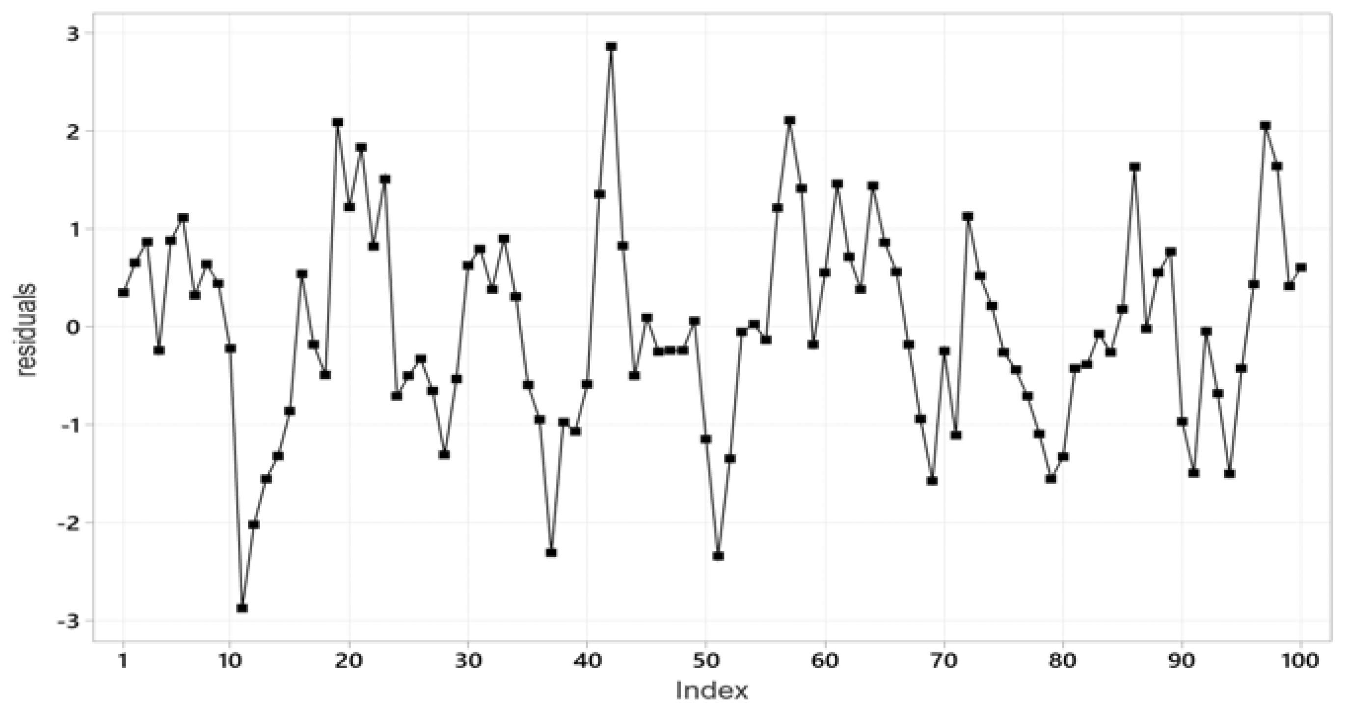
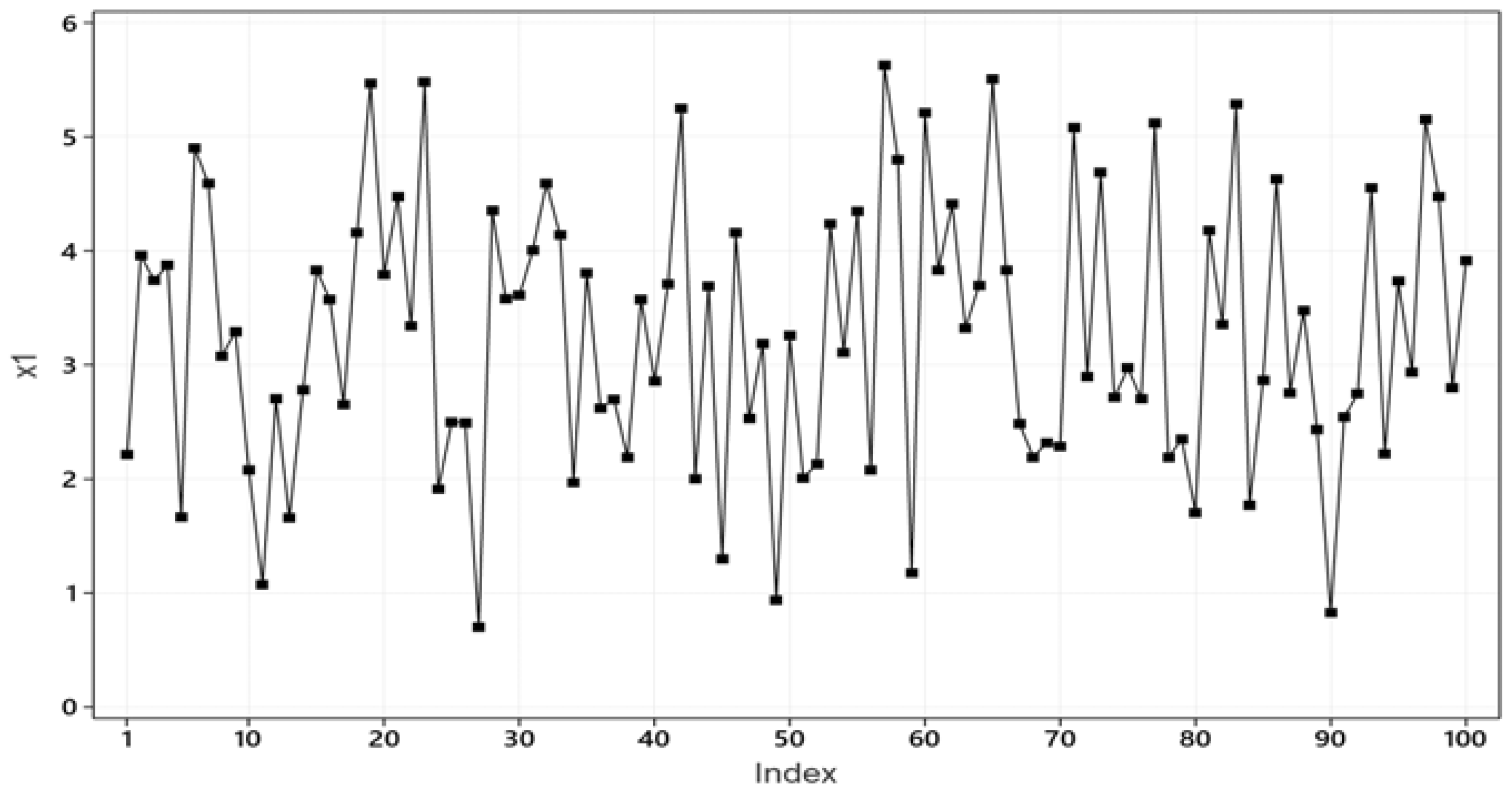
To answer that one needs to evaluate the statistical adequacy of both estimated models in (20) using informal t-plots of the data combined with formal M-S testing (Spanos [19]) to probe their statistical adequacy. The t-plot for data ${\mathbf{x}}_1$ (Figure 1) exhibits no obvious departures from the NIID assumptions, but the ‘irregular cycles’ exhibited by ${\mathbf{x}}_2$ (Figure 2) indicate a likely departures from ‘Independence’.

The validity of the IID assumptions can be tested using the runs test (Spanos, 2019) [18]:

$$\begin{array}{c}{d}_R\left(\mathbf{X}\right)={\displaystyle \frac{\left[E\left(R\right)-R\right]}{\sqrt{Var\left(R\right)}}}\stackrel{\mathrm{IID}}{\approx }\mathsf{N}(0,1),d_R\left(\mathbf{X}\right)\stackrel{\mathrm{non}-\mathrm{IID}}{\backsim }\mathsf{N}({\delta }_n,{\tau }_n^2),{\delta }_n\ne 0,{\tau }_n^2>0,\end{array}$$

(21)

where R-number of runs, $E\left(R\right)={\displaystyle \frac{2n-1}{3}},Var\left(R\right)={\displaystyle \frac{16n-29}{90}}$, ${\delta }_n$ and ${\tau }_n^2$ depend only on $n.$ The Anderson-Darling (A-D) tests for Normality are also given in

Table 7. Simple M-S tests for IID.

Data	Runs Test for IID	Normality Test
${\mathbf{x}}_1$:	$d_R\left({\mathbf{x}}_1\right)={\displaystyle \frac{(50-51)}{4.178}}=0.239\left[0.918\right]$	A-$D\left({\mathbf{x}}_1\right)=0.414\left[0.330\right]$
${\mathbf{x}}_2$:	$d_R\left({\mathbf{x}}_2\right)={\displaystyle \frac{(32-51)}{4.178}}=4.548\left[0.000\right]$	A-$D\left({\mathbf{x}}_2\right)=0.177\left[0.918\right]$

.

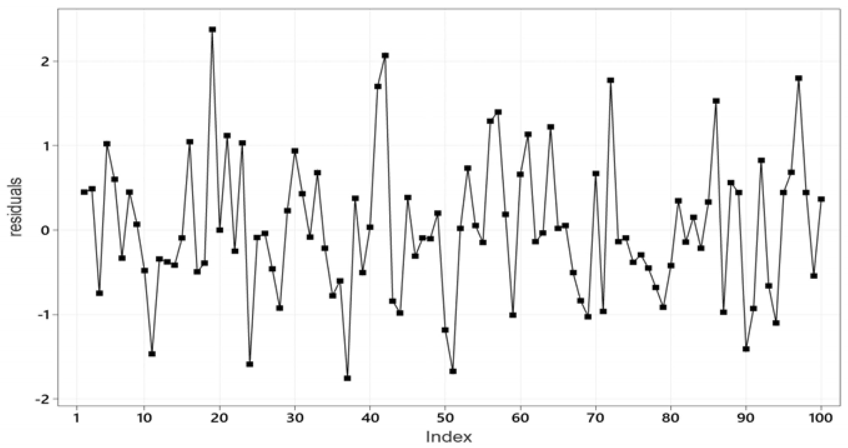
The M-S testing results in Table 7 confirm that the simple Normal model in (2) is statistically adequate for data ${\mathbf{x}}_1$, but misspecified with data ${\mathbf{x}}_2$ since the ‘Independence’ assumption is invalid. This is corroborated by the t-plot of the residuals $\{{\widehat{u}}_{2t},$ $t=1,2,...,n\}$ in Figure 3, which exhibits similar irregular cycles as Figure 2. This implies that the inference results in Table 6 based on ${\mathbf{x}}_2$ will be unreliable since the non-independence induces sizeable discrepancies between the actual and nominal error probabilities; see Spanos [18].

Thus, the results based on data ${\mathbf{x}}_2$ do not represent a successful replication (with trustworthy evidence) of those based on data ${\mathbf{x}}_1$. To secure trustworthy evidence for any inferential claim using data ${\mathbf{x}}_2$ one needs to respecify the original ${\mathcal{M}}_{\mathit{\theta }}\left(\mathbf{x}\right)$ in (2) by selecting an alternative statistical model ${\mathcal{M}}_{\mathit{\theta }}\left({\mathbf{x}}_2\right)$ aiming to account for the dependence mirrored by the irregular cycles in Figure 2 and Figure 3.

An obvious choice in this case is to replace the assumptions of IID with Markov dependence and stationarity, which give rise to an Autoregressive [AR(1)] model; see Spanos [18]. Estimating the AR(1) model with data ${\mathbf{x}}_2$ yields:

$$\begin{array}{c}{X}_{2t}=\underset{\left(0.278\right)}{1.331}+\underset{\left(0.083\right)}{0.583} X_{2t-1}+{\widehat{v}}_{2t},s_2=0.874.\end{array}$$

(22)

The t-plot of the residuals $\{{\widehat{v}}_{2t},$ $t=1,2,\dots ,n\}$ from (22) in Figure 4 indicates that the Markov dependence assumption accounts for the irregular cycles exhibited by the residuals in Figure 2 and Figure 3. The statistical adequacy of (22) is confirmed by the M-S tests:

$$\begin{array}{c}{d}_R\left({\mathbf{v}}_2\right)={\displaystyle \frac{(51-50.1)}{4.157}}=0.217\left[0.853\right],A-D\left({\mathbf{v}}_2\right)=0.438\left[0.290\right].\end{array}$$

4.2. Fallacious Evidential Interpretations of Inference Results

Another crucial source of the untrustworthiness of evidence is unwarranted and fallacious evidential interpretations of unduly data-specific inference results as evidence for particular inferential claims.

Example 1 (continued). The optimality of the point estimators,

$\widehat{\mu }\left(\mathbf{X}\right)={\overline{X}}_n={\displaystyle \frac{1}{n}}{\sum }_{t=1}^n{X}_t$, $s^2\left(\mathbf{X}\right)={\displaystyle \frac{1}{(n-1)}}{\sum }_{t=1}^n{(X_t-{\overline{X}}_n)}^2,$does not entail:

$$\begin{array}{c}\hfill \widehat{\mu }\left({\mathbf{x}}_0\right)\simeq {\mu }^{*}, \mathrm{and}{s}^2\left({\mathbf{x}}_0\right)\simeq {\sigma }_{*}^2, \mathrm{for} n \mathrm{large} \mathrm{enough},\end{array}$$

(23)

where ≃ indicates approximate equality. The claims in (23) are unwarranted since $\widehat{\mu }\left({\mathbf{x}}_0\right)$ and $s^2\left({\mathbf{x}}_0\right)$ ignore the relevant uncertainty associated with $\widehat{\mu }\left({\mathbf{x}}_0\right)$ and $s^2\left({\mathbf{x}}_0\right)$ rely exclusively on single point, $\mathbf{X}={\mathbf{x}}_0$ from the sampling distributions, $f(\widehat{\mu }\left(\mathbf{x}\right);\theta )$ and$f(s^2\left(\mathbf{x}\right);\theta ),\forall \mathbf{x}\in {\mathbb{R}}^n$; see Spanos [16]. Invoking asymptotic properties for $\widehat{\mu }\left(\mathbf{X}\right)$ and $s^2\left(\mathbf{X}\right),$ such as consistency, will not justify the claims in (23). As argued by Le Cam [40] p. xiv: “... limit theorems ‘as n tends to infinity’ are logically devoid of content about what happens at any particular n”.

(b) It is important to emphasize that the problem with the claim $\widehat{\theta }\left({\mathbf{x}}_0\right)\simeq {\theta }^{*}$ also extends to estimation-based effect sizes; see Ellis [41]. For instance, in the case of testing the differences between two means, Cohen’s $d={\displaystyle \frac{({\overline{x}}_n-{\overline{y}}_n)}{s}}$ is nothing more than

an estimate $h\left({\mathbf{z}}_0\right)={\displaystyle \frac{({\overline{x}}_n-{\overline{y}}_n)}{s}}$ relating to the estimator $h\left(\mathbf{Z}\right)={\displaystyle \frac{({\overline{X}}_n-{\overline{Y}}_n)}{s}}$ of $h\left(\mathit{\theta }\right)={\displaystyle \frac{({\mu }_1-{\mu }_2)}{\sigma }}$

In that sense, the claim that ${\displaystyle \frac{({\overline{x}}_n-{\overline{y}}_n)}{s}}\simeq {\displaystyle \frac{({\mu }_1^{*}-{\mu }_2^{*})}{{\sigma }_{*}}}$ is a variation on the same unwarranted claim: $\widehat{\theta }\left({\mathbf{x}}_0\right)\simeq {\theta }^{*}$for n large enough; see Spanos [16]

(c) The inferential claim associated with (5) relates to the random CI$(\mathbf{X};\mu )$ overlaying ${\mu }^{*}$ with probability $(1-\alpha ),$ but does not extend to $CI\left({\mathbf{x}}_0\right)$ Spanos [16]:

$$\begin{array}{c}\hfill CI\left({\mathbf{x}}_0\right)=[{\overline{x}}_n-c_{\frac{\alpha }{2}}(s\left({\mathbf{x}}_0\right)/\sqrt{n}),{\overline{x}}_n+c_{\frac{\alpha }{2}}\left(s\left({\mathbf{x}}_0\right)\right].\end{array}$$

(24)

As Neyman [42], p. 288, argued: “…valid probability statements about random variables usually cease to be valid if the random variables are replaced by their particular values”. i.e., the factual reasoning makes no sense post-data [${\mathbf{x}}_0$ has occurred].

(d) It is also well-known that interpreting the ‘accept/reject $H_0$ results’ as evidence for $H_0$/$H_1$ is unsound giving rise to two related fallacies (Mayo and Spanos [14]):

Fallacy of acceptance: misinterpreting ‘accept $H_0$’ (no evidence against $H_0$) as evidence for $H_0$’. This could easily arise in cases where n is too small and the test has no sufficient power to detect a actual discrepancy ${\gamma }_1={\theta }_0-{\theta }_1\pm 0$.

Fallacy of rejection: misinterpreting ‘reject $H_0$’ (evidence against $H_0$) as evidence for a particular $H_1$’. This could easily arise when n is very large and the test is sensitive enough to detect tiny discrepancies; see Spanos [43].

The above arguments call into question the M-PPV-inspired reforms relating to replacing p-values with CIs and effect sizes, and redefining statistical significance by reducing the conventional thresholds for $\alpha$, as ill-thought-out.

5. Testing Results vs. the Post-Data Severity (SEV) Evaluation

The reason why the accept/reject $H_0$ results are not routinely replicable with akin data is that they are sensitive to (i) the framing of $H_0$ and $H_1$, (ii) the prespecified $\alpha$ and (iii) the sample size n. A principled procedure transmuting the unduly data-dependent accept/reject $H_0$ results into evidence relating to ${\theta }^{*}$ is the post-data severity (SEV) evaluation, guided by the sign and magnitude of $d\left({\mathbf{x}}_0\right)$. A hypothesis H ($H_0$ or $H_1$) passes a severe test $T_{\alpha }$ with data ${\mathbf{x}}_0$ if (Mayo and Spanos [14]):

(C-1)

${\mathbf{x}}_0$ accords with H, and

(C-2)

with very high probability, test $T_{\alpha }$ would have produced a result that ‘accords less well’ with H than ${\mathbf{x}}_0$ does, if H were false.

5.1. Case 1: Reject $H_0$

Example 6. Consider the simple Bernoulli model:

$$\begin{array}{c}\hfill X_k\backsim \mathsf{BerIID}(\theta ,\theta (1-\theta )),x_k=0,1,0<\theta <1,k\in \mathbb{N},\end{array}$$

(25)

where $\theta =E\left(X_k\right)=\mathbb{P}(X_k=1),$ and the hypotheses:

$$\begin{array}{c}{H}_0:\theta \le {\theta }_0\mathrm{vs}.H_1:\theta >{\theta }_0,\mathrm{for}{\theta }_0=0.5\end{array}$$

(26)

It can be shown that the t-type test (Lehmann and Romano, [20]):

$$\begin{array}{c}\hfill T_{\alpha }^{>}:=\{d\left(\mathbf{X}\right)={\displaystyle \frac{\sqrt{n}({\overline{X}}_n-{\theta }_0)}{\sqrt{{\theta }_0(1-{\theta }_0)}}},{\mathcal{C}}_1\left(\alpha \right)=\{\mathbf{x}:d\left(\mathbf{x}\right)>c_{\alpha }\},\mathrm{for} {\overline{X}}_n={\displaystyle \frac{1}{n}}{\sum }_{i=1}^n{X}_i,\end{array}$$

(27)

is optimal in the sense of Uniformly Most Powerful (UMP). The sampling distribution of $d\left(\mathbf{X}\right)$ evaluated under $H_0$ (hypothetical: what if $\theta ={\theta }_0$) is:

$$\begin{array}{c}d\left(\mathbf{X}\right)={\displaystyle \frac{\sqrt{n}({\overline{X}}_n-{\theta }_0)}{\sqrt{{\theta }_0(1-{\theta }_0)}}}\stackrel{\theta ={\theta }_0}{\backsim }\mathsf{Bin}\left(0,1;n\right)\simeq \mathrm{N}(0,1),\end{array}$$

(28)

where the ‘scaled’ Binomial distribution, $\mathsf{Bin}\left(0,1;n\right),$ can be approximated (≃) by the N$(0,1)$, which is used to evaluate $\alpha$ and the p-value:

$$\begin{array}{cc}\alpha =\mathbb{P}(d\left(\mathbf{X}\right)>c_{\alpha };\theta ={\theta }_0),\hfill & p\left({\mathbf{x}}_0\right)=\mathbb{P}(d\left(\mathbf{X}\right)>d\left({\mathbf{x}}_0\right);\theta ={\theta }_0).\hfill \end{array}$$

(29)

The sampling distribution of $d\left(\mathbf{X}\right)$ under $H_1$ (hypothetical: what if $\theta ={\theta }_1$) is:

$$\begin{array}{c}d\left(\mathbf{X}\right)={\displaystyle \frac{\sqrt{n}({\overline{X}}_n-{\theta }_0)}{\sqrt{{\theta }_0(1-{\theta }_0)}}}\stackrel{\theta ={\theta }_1}{\backsim }\mathsf{Bin}\left(\delta \left({\theta }_1\right),\sqrt{V\left({\theta }_1\right)};n\right),\mathrm{for}{\theta }_1={\theta }_0+{\gamma }_1,{\gamma }_1\ge 0,\\ \delta \left({\theta }_1\right)={\displaystyle \frac{\sqrt{n}({\theta }_1-{\theta }_0)}{\sqrt{{\theta }_0(1-{\theta }_0)}}},V\left({\theta }_1\right)={\displaystyle \frac{{\theta }_1(1-{\theta }_1)}{{\theta }_0(1-{\theta }_0)}},\end{array}$$

(30)

whose probabilities can be approximated using:

$$\begin{array}{c}{\left(\sqrt{V\left({\theta }_1\right)}\right)}^{-1}\left[d\left(\mathbf{X}\right)-\delta \left({\theta }_1\right)\right]\stackrel{\theta ={\theta }_1}{\backsim }\mathsf{Bin}\left(0,1;n\right)\simeq \mathsf{N}(0,1).\end{array}$$

(31)

(31) is used to derive the type II error and the power of the test $T_{\alpha }^{>}$ in (27) which increases monotonically with $\sqrt{n}$ and $\left({\mu }_1-{\mu }_0\right)$ and decreases with $V\left({\theta }_1\right)$.

Example 6 (continued). For the simple Bernoulli model in (25), the relevant data ${\mathbf{x}}_0$ refer to newborns for 2020 in Cyprus, 5190 male $\left(X=1\right)$ and 4740 female $\left(X=0\right)$, i.e., $n=9930$. The optimal test$T_{\alpha }^{>}$ in (27), based on $\alpha =0.001$ and ${\widehat{\theta }}_n\left({\mathbf{x}}_0\right)=0.523,$ yields:

$$\begin{array}{c}\hfill d\left({\mathbf{x}}_0\right)=4.5158,\mathrm{indicating} ‘\mathrm{reject} H_0’ \mathrm{with} p\left({\mathbf{x}}_0\right)=0.000003.\end{array}$$

This, combined with $d\left({\mathbf{x}}_0\right)>0,$ suggest that condition C-1 implies that ${\mathbf{x}}_0$ accords with $H_1$, and condition C-2 indicates that the relevant event relates to: “outcomes $\mathbf{x}$ that accord less well with $\theta >{\theta }_1$ than ${\mathbf{x}}_0$ does”, i.e., event $\{\mathbf{x}$: $d\left(\mathbf{x}\right)\le d\left({\mathbf{x}}_0\right)\},\forall \mathbf{x}\in {\{0,1\}}^n,$ and its probability relates to the inferential claim $\theta >{\theta }_1={\theta }_0+{\gamma }_1,$${\gamma }_1>0$:

$$\begin{array}{c}SE{V}_R(T_{\alpha }^{>};\theta >{\theta }_1)=\underset{{\theta }_1\in {\Theta }_1}{\sup }\mathbb{P}(d\left(\mathbf{X}\right)\le d\left({\mathbf{x}}_0\right);\theta ={\theta }_1)=p_1,\end{array}$$

(32)

where ${\Theta }_1=(0.5,1),$ $p_1>0.5$ is a prespecified (high enough) probability. The evaluation of (32), based on (31) gives rise to the severity curve depicted in Figure 5, assigning probabilities relating to the warrant with data ${\mathbf{x}}_0$ of different discrepancies ${\gamma }_1=({\theta }_1-{\theta }_0)>0$.

The largest discrepancy $\gamma$ warranted with severity $0.9$ by test $T_{\alpha }^{>}$ and data ${\mathbf{x}}_0$ is ${\gamma }^{‡}\le 0.01623({\theta }_1^{‡}=0.51623);$ see

Table 8. $SEV(T_{\alpha }^{>};\theta :={\theta }_1)$ for ‘reject ${\theta }_0=0.5$’ and ‘accept ${\theta }_0=(18/35)$’ with ($T_{\alpha }^{>};{\mathbf{x}}_0)$.

${\theta }_0=0.5$: ${\gamma }_1=$	0.01	0.013	0.015	0.0155	0.01623	0.017	0.018	0.02265	0.025	0.03
${\theta }_0=\left({\displaystyle \frac{18}{35}}\right)$: ${\gamma }_1=$	***	***	***	0.0012	0.0019	0.0027	0.0037	0.0084	0.011	0.016
${\theta }_1=$	0.51	0.513	0.515	0.5155	0.51623	0.517	0.518	0.52265	0.525	0.53
$\mathsf{Sev}(\theta :={\theta }_1)=$	0.994	0.973	0.937	0.923	0.900	0.870	0.824	0.500	0.320	0.071

*** indicate “no entry”.

. How does the post-data SEV evaluation convert the unduly data-specific accept/reject $H_0$ results into evidence, giving rise to learning from data ${\mathbf{x}}_0$ about ${\theta }^{*}?$ While the SEV evaluation is always attached to $T_{\alpha }^{>}$in (27), as it relates to the relevant inferential claim $\theta >{\theta }_1$, ${\gamma }^{‡}\le 0.01623({\theta }_1^{‡}=0.51623)$ warranted with probability $0.9,$ could be viewed as narrowing down the coarse accept/reject $H_0$ result indicating that ${\theta }^{*}\in (0.5,1)$ to the much narrower ${\theta }^{*}\in (0.516\pm \epsilon )$ for $0<\epsilon \le 0.0002$.

5.2. Case 2: Accept $H_0$

Example 6 (continued). Consider replacing ${\theta }_0=0.5$ in (26) with the Nicholas Bernoulli value ${\theta }_0=(18/35)\simeq 0.5143$. Applying the UMP test$T_{\alpha }^{>}$ yields:

$$\begin{array}{c}\hfill d_B\left({\mathbf{x}}_0\right)=1.669,\mathrm{with} a p-\mathrm{value} p\left({\mathbf{x}}_0\right)=0.0476,\end{array}$$

indicating ‘accept $H_0$’ at $\alpha =0.001,$ but given $d_B\left({\mathbf{x}}_0\right)>0,$ the relevant $SE{V}_A(T_{\alpha }^{>};\theta >{\theta }_1)$ for the inferential claim, $\theta >{\theta }_1={\theta }_0+{\gamma }_1,$ ${\gamma }_1>0,$ is:

$$\begin{array}{c}SE{V}_A(T_{\alpha }^{>};\theta >{\theta }_1)=\underset{{\theta }_1\in {\Theta }_1}{inf}\mathbb{P}(d\left(\mathbf{X}\right)\le d\left({\mathbf{x}}_0\right);\theta ={\theta }_1)=p_1>0.5,\end{array}$$

(33)

whose evaluation is based on (31), which is identical to that of rejecting $H_0$ based on ${\theta }_0=0.5,$ in Figure 5, despite the change of the result from reject to accept ${\theta }_0=(18/35)$! Indeed, comparing the results for $SE{V}_R(T_{\alpha }^{>};\theta >{\theta }_1)$ and $SE{V}_A(T_{\alpha }^{>};\theta :={\theta }_1)$ in Table 8, is clear that even though the discrepancies ${\gamma }_1$ are different (${\theta }_0=0.5$,${\theta }_0=(18/35)),$ the two curves are identical $\forall {\theta }_1\in (0.5,1)$. As a result, for the same inferential claim, $\theta :={\theta }_1={\theta }_0+{\gamma }_1,$ ${\gamma }_1:=0,$ the largest discrepancy ${\gamma }_1:=0$ at $0.9$ probability from ${\theta }_0=0.5$ (reject $H_0$) coincides with the smallest discrepancy ${\gamma }_1$ from ${\theta }_0=(18/35)$ (accept $H_0$). Also, the low severity ($0.5$) for the point estimate ${\widehat{\theta }}_n\left({\mathbf{x}}_0\right)=0.52266$ ensures that $\gamma =0.02266$ will never be a warranted discrepancy, i.e., there is strong evidence against the claim ${\widehat{\theta }}_n\left({\mathbf{x}}_0\right)\simeq 0.52266$.

What renders the SEV evaluation different is that it calibrates the warranted ${\gamma }_1^{‡},$ with high enough probability. In that sense, it can be viewed as a testing-based effect size that provides a more reliable evaluation of the ‘scientific effect’; see Spanos [16]. This should contrasted with the estimation-based effect size measure, $({\widehat{\theta }}_n\left({\mathbf{x}}_0\right)-0.5)/\sqrt{0.5(1-0.5)}=0.045$ (Ellis, 2010) [41], which is equally fallacious as that claim that ${\widehat{\theta }}_n\left({\mathbf{x}}_0\right)\simeq {\theta }^{*}$ for n large enough.

Statistical vs. substantive significance. The SEV evaluation would also address this problem by relating the discrepancy ${\gamma }^{‡}$ from ${\theta }_0$ (${\theta }_1={\theta }_0\pm {\gamma }^{‡}$) warranted by test $T_{\alpha }$ and data ${\mathbf{x}}_0$ with high probability to the substantively determined value ${\phi }^{⧫}$. For example, in human biology (Hardy, [44]) it is known that the substantive value for the ratio of boys to all newborns is ${\phi }^{⧫}\simeq 0.5122$. Comparing ${\phi }^{⧫}$ with the severity-based warranted discrepancy, ${\gamma }_1^{‡}\le$0.01556 (${\theta }_1\le 0.51623$) suggests that the statistically determined ${\gamma }_1^{‡}$ includes the substantive value since ${\phi }^{⧫}\simeq 0.5122<0.51623$. In fact, the SEV evaluation of ${\theta }_1\le 0.5122$ is $0.981$.

5.3. Post-Data Severity and the Trustworthiness of Evidence

The above discussion suggests that similar point estimates, observed CIs, and testing results do not guarantee a successful replication or/and trustworthy evidence. Although the statistical adequacy of the underlying statistical models is necessary, it is not sufficient, especially when the sample size n of such studies is different.

An obvious way to address this issue is to use the distinction between statistical results and evidence and compare the warranted discrepancies $\gamma$ from the null value, $\theta ={\theta }_0$ by the tests in question with high enough severity. To illustrate, consider an example that utilizes similar data from two different countries, three centuries apart.

Example 6 (continued). To bring out the replicability of the SEV evidential claims, consider data ${\mathbf{x}}_1$ that refer to newborns during 1668 in London (England), 6073 boys, 5560 girls, $n=11,633$ (Arbuthnot [45]), 352 years before the Cyprus 2020 data. The optimal test in (27) yields $d\left({\mathbf{x}}_1\right)=4.756,$ with $p\left({\mathbf{x}}_1\right)=0.0000001,$ rejecting $H_0$: $\theta \le 0.5.$ This result is close to $d\left({\mathbf{x}}_0\right)=4.5158,$ with $p\left({\mathbf{x}}_0\right)=0.000003$ from Cyprus for 2020, but the question of interest is whether the latter constitutes a successful replication of the 1668 data. Using $SEV(T_{\alpha }^{>};{\mathbf{x}}_1;\theta >{\theta }_1)=0.9$, the warranted discrepancy from ${\theta }_0=0.5$ by test $T_{\alpha }^{>}$ and London data ${\mathbf{x}}_1$ is ${\gamma }_1^{‡}\le 0.0161$ which is almost identical to that with the Cyprus data ${\gamma }_0^{‡}\le 0.0162$, affirming the replicability of the evidence that ${\theta }^{*}\in (0.5,0.516]$.

The two severity curves in Figure 6 for data ${\mathbf{x}}_0$ and ${\mathbf{x}}_1$ are almost identical for the range of values of $\theta$ that matters ($SEV(T_{\alpha }^{>};{\mathbf{x}}_0;\theta >{\theta }_1)>0.8$), despite the fact that $n=9930$ vs. $n=11,633.$ Hence, for a statistically adequate ${\mathcal{M}}_{\mathit{\theta }}\left(\mathbf{x}\right)$, the SEV could provide a more robust measure of replicability of trustworthy evidence, than point estimates, effect sizes, observed CIs, or p-values; see Spanos [16].

The key to enabling the $SEV(T_{\alpha }^{>};{\mathbf{x}}_0;\theta >{\theta }_1)$ evaluation to circumvent the problem with different sample sizes n is that the two components in $\left[d\left({\mathbf{x}}_0\right)-\delta \left({\theta }_1\right)\right]$ use the same n to evaluate the discrepancy ${\gamma }_1={\theta }_1-{\theta }_0\ge 0$, addressing the above-mentioned fallacies of acceptance and rejection. In contrast, the power of $T_{\alpha }^{>}$ is evaluated using $\left[c_{\alpha }-\delta \left({\theta }_1\right)\right],$ where $c_{\alpha }$ is based on the prespecified $\alpha ,$ and the p-valueis evaluated only under $\theta ={\theta }_0$, $d\left(\mathbf{X}\right)\stackrel{\theta ={\theta }_0}{\backsim }$N$(0,1)$, rendering both evaluations vulnerable to the large/small n problems.

The SEV can be used to address other foundational problems, including distinguishing between statistical and substantive significance, as well as providing a testing-based effect size for the magnitude of the ‘substantive’ effect. An example of that is illustrated in Spanos (2023) [17], where a published paper reports a t-test for an estimated regression coefficient $\widehat{\beta }=0.004$ claimed to be significant at $\alpha =0.05$ with $n=24,732,966$ and a p-value $p=0.045$. The SEV evalution of that claim indicates that the warranted magnitude of the coefficient would be considerably smaller at $\beta \le 0.00000001$ with high enough severity.

6. Summary and Conclusions

The case made by Ioannidis [1], based on M-PPV misrepresents frequentist testing and misdiagnoses the replication crisis, due to the its incongruous stipulations [S1]–[S2] based on highly questionable presuppositions [a]–[d]. The most ill-chosen incongruousness is the colligating of the false positive/negative with the type I/II error probabilities. This led to promoting ill-informed reforms, including replacing p-values with CIs and effect sizes and lowering $\alpha$.

The above discussion has made a case that the non-replicability and the untrustworthiness of empirical evidence stem primarily from the uninformed and recipe-like implementation of statistical modeling and inference. This ignores fundamental issues relating to (a) establishing the statistical adequacy of the invoked statistical model ${\mathcal{M}}_{\mathit{\theta }}\left(\mathbf{x}\right)$ for data ${\mathbf{x}}_0$, (b) the reasoned implementation of frequentist inference and the pertinent interpretation of their error probabilities, as well as (c) warranted evidential interpretations of inference results. Fisher’s model-based statistics provides an incisive explanation for the non-replication/untrustworthiness of empirical evidence and an appropriate framework for addressing (a)–(c). The statistical adequacy of ${\mathcal{M}}_{\mathit{\theta }}\left(\mathbf{x}\right)$ is necessary for securing the trustworthiness of empirical evidence and ensuring the crucial link between trustworthiness and replicability, as both are key aspects firmly attached to individual studies. The inveterate problem with frequentist testing is that the accept/reject $H_0$ results are too coarse and unduly data-specific to provide cogent evidence for ${\theta }^{*}.$ This problem can be addressed using their post-data SEV evaluation to output the discrepancy ${\gamma }_1=({\theta }_1-{\theta }_0)$ warranted by data ${\mathbf{x}}_0$ with high probability, which narrows down the coarseness of these results. From this perspective, abuses of frequentist testing represents the tip of the untrustworthy evidence iceberg, with the remainder stemming mainly from statistical/substantive misspecification.

As Stark and Saltelli [12] aptly argue: “The problem is one of cargo-cult statistics – the ritualistic miming of statistics rather than conscientious practice. This has become the norm in many disciplines, reinforced and abetted by statistical education, statistical software, and editorial policies” (p. 40).

A redeeming value of the Ioannidis [1] case might be that its provocative title raised awareness of the endemic untrustworthiness of published empirical evidence. This could potentially initiate a fertile dialogue leading to ameliorating this thorny problem. This could happen when the focus is redirected to the reasoned implementation of frequentist modeling and inference guided by statistical adequacy. That is, replicating influential empirical papers in a particular research area with the same or akin data, and evaluating their statistical and substantive adequacy, represents the most effective way to establish the untrustworthiness of published empirical evidence.

The endemic untrustworthiness of published empirical evidence in most disciplines could be redressed but would require a lot of difficult changes, including: (i) a substantial overhaul of the teaching of probability theory and statistics, (ii) crucial changes in the current statistical software to include M-S testing, and (iii) changes in the editorial policies for papers that rely on statistical inference requiring corroboration of the statistical adequacy for the invoked statistical models.

References

1. Ioannidis, J.P.A. Why most published research findings are false. PLoS Med. 2005, 2, e124. [Google Scholar] [CrossRef] [PubMed]
2. Baker, M. Reproducibility crisis. Nature 2016, 533, 353–366. [Google Scholar]
3. Hoffler, J.H. Replication and Economics Journal Policies. Am. Econ. Rev. 2017, 107, 52–55. [Google Scholar] [CrossRef]
4. Wasserstein, R.L.; Schirm, A.L.; Lazar, N.A. Moving to a world beyond ‘p < 0.05’. Am. Stat. 2019, 73, 1–19. [Google Scholar]
5. Simmons, J.P.; Nelson, L.D.; Simonsohn, U. False-Positive Psychology: Undisclosed Flexibility in Data Collection and Analysis Allow Presenting Anything as Significant. Psychol. Sci. 2011, 22, 1359–1366. [Google Scholar] [CrossRef]
6. Camerer, C.F.; Dreber, A.; Forsell, E.; Ho, T.H.; Huber, J.; Johannesson, M.; Kirchler, M.; Almenberg, J.; Altmejd, A.; Chan, T.; et al. Evaluating replicability of laboratory experiments in economics. Science 2016, 351, 1433–1436. [Google Scholar] [CrossRef]
7. Benjamin, D.J.; Berger, J.O.; Johannesson, M.; Nosek, B.A.; Wagenmakers, E.J.; Berk, R.; Bollen, K.A.; Brembs, B.; Brown, L.; Camerer, C.; et al. Redefine statistical significance. Nat. Hum. Behav. 2017, 33, 6–10. [Google Scholar] [CrossRef]
8. Shrout, P.E.; Rodgers, J.L. Psychology, science, and knowledge construction: Broadening perspectives from the replication crisis. Annu. Rev. Psychol. 2018, 69, 487–510. [Google Scholar] [CrossRef]
9. Johnson, V.E.; Payne, R.D.; Wang, T.; Asher, A.; Mandal, S. On the Reproducibility of Psychological Science. J. Am. Stat. Assoc. 2017, 112, 1–10. [Google Scholar] [CrossRef]
10. Andreou, E.; Spanos, A. Statistical adequacy and the testing of trend versus difference stationarity. Econom. Rev. 2003, 22, 217–237. [Google Scholar] [CrossRef]
11. Do, H.P.; Spanos, A. Revisiting the Phillips curve: The empirical relationship yet to be validated. Oxf. Bull. Econ. Stat. 2024, 86, 761–794. [Google Scholar] [CrossRef]
12. Stark, P.B.; Saltelli, A. Cargo-cult statistics and scientific crisis. Significance 2018, 15, 40–43. [Google Scholar] [CrossRef]
13. Fisher, R.A. On the mathematical foundations of theoretical statistics. Philos. Trans. R. Soc. A 1922, 222, 309–368. [Google Scholar]
14. Mayo, D.G.; Spanos, A. Severe Testing as a Basic Concept in a Neyman-Pearson Philosophy of Induction. Br. J. Philos. Sci. 2006, 57, 323–357. [Google Scholar] [CrossRef]
15. Nickerson, R.S. Null Hypothesis Significance Testing: A review of an old and continuing controversy. Psychol. Methods 2000, 5, 241–301. [Google Scholar] [CrossRef] [PubMed]
16. Spanos, A. Revisiting noncentrality-based confidence intervals, error probabilities, and estimation-based effect sizes. J. Math. Stat. Psychol. 2021, 104, 102580. [Google Scholar] [CrossRef]
17. Spanos, A. Revisiting the Large n (Sample Size) Problem: How to Avert Spurious Significance Results. Stats 2023, 6, 1323–1338. [Google Scholar] [CrossRef]
18. Spanos, A. Probability Theory and Statistical Inference: Empirical Modeling with Observational Data; Cambridge University Press: Cambridge, UK, 2019. [Google Scholar]
19. Spanos, A. Mis-Specification Testing in Retrospect. J. Econ. Surv. 2018, 32, 541–577. [Google Scholar] [CrossRef]
20. Lehmann, E.L.; Romano, J.P. Testing Statistical Hypotheses; Springer: New York, NY, USA, 2005. [Google Scholar]
21. Neyman, J.; Pearson, E.S. On the problem of the most efficient tests of statistical hypotheses. Philos. Trans. R. A 1933, 231, 289–337. [Google Scholar]
22. Bennett, J.H. Statistical Inference and Analysis: Selected Correspondence of RA Fisher; Clarendon Press: Oxford, UK, 1990. [Google Scholar]
23. Gigerenzer, G. The superego, the ego, and the id in statistical reasoning. In A Handbook for Data Analysis in the Behavioral Sciences: Methodological Issues; Psychology Press: London, UK, 1993; pp. 311–339. [Google Scholar]
24. Halpin, P.F.; Stam, J.H. Inductive Inference or Inductive Behavior: Fisher and Neyman: Pearson Approaches to Statistical Testing in Psychological Research (1940–1960). Am. J. Psychol. 2006, 119, 625–653. [Google Scholar] [CrossRef]
25. Fisher, R.A. Properties of Hh functions. In Introduction to the British Association of Mathematical Tables; British Association: London, UK, 1931; Volume 1, p. 26. [Google Scholar]
26. Fisher, R.A. The Design of Experiments; Oliver and Boyd: Edinburgh, UK, 1935. [Google Scholar]
27. Box, J.F. R.A. Fisher, The Life of a Scientist; Wiley: New York, NY, USA, 1978. [Google Scholar]
28. Yerushalmy, J. Statistical problems in assessing methods of medical diagnosis, with special reference to X-ray techniques. Public Health Rep. (1896–1970) 1947, 62, 1432–1449. [Google Scholar] [CrossRef]
29. Neyman, J. Outline of statistical treatment of the problem of diagnosis. Public Health Rep. (1896–1970) 1947, 62, 1449–1456. [Google Scholar] [CrossRef]
30. Spanos, A. Is Frequentist Testing Vulnerable to the Base-Rate Fallacy? Philos. Sci. 2010, 77, 565–583. [Google Scholar] [CrossRef]
31. Bishop, Y.V.; Fienberg, S.E.; Holland, P.W. Discrete Multivariate Analysis; MIT Press: Cambridge, MA, USA, 1975. [Google Scholar]
32. Senn, S. Statistical Issues in Drug Development, 3rd ed.; Wiley: New York, NY, USA, 2021. [Google Scholar]
33. Greenhouse, S.W.; Mantel, N. The evaluation of diagnostic tests. Biometrics 1950, 6, 399–412. [Google Scholar] [CrossRef]
34. Nissen-Meyer, S. Evaluation of screening tests in medical diagnosis. Biometrics 1964, 20, 730–755. [Google Scholar] [CrossRef]
35. Freedman, D.; Pisani, R.; Purves, R. Statistics, 3rd ed.; Norton: New York, NY, USA, 1998. [Google Scholar]
36. Nosek, B.A.; Hardwicke, T.E.; Moshontz, H.; Allard, A.; Corker, K.S.; Dreber, A.; Fidler, F.; Hilgard, J.; Struhl, M.K.; Nuijten, M.B.; et al. Replicability, robustness, and reproducibility in psychological science. Annu. Rev. Psychol. 2022, 73, 719–748. [Google Scholar] [CrossRef]
37. Munafò, M.R.; Nosek, B.A.; Bishop, D.V.M.; Button, K.S.; Chambers, C.D.; Percie du Sert, N.; Simonsohn, U.; Wagenmakers, E.J.; Ware, J.J.; Ioannidis, J.P.A. A manifesto for reproducible science. Nat. Hum. Behav. 2017, 1, 1–9. [Google Scholar] [CrossRef]
38. Bird, A. Understanding the Replication Crisis as a Base Rate Fallacy. Br. J. Philos. Sci. 2021, 72, 965–993. [Google Scholar] [CrossRef]
39. Leek, J.T.; Peng, R.D. Statistics: P values are just the tip of the iceberg. Nature 2015, 520, 520–612. [Google Scholar] [CrossRef]
40. Le Cam, L. Asymptotic Methods in Statistical Decision Theory; Springer: New York, NY, USA, 1986. [Google Scholar]
41. Ellis, P.D. The Essential Guide to Effect Sizes: Statistical Power, Meta-Analysis, and the Interpretation of Research Results; CUP: Cambridge, UK, 2010. [Google Scholar]
42. Neyman, J. Note on an article by Sir Ronald Fisher. J. R. Stat. Ser. B 1956, 18, 288–294. [Google Scholar] [CrossRef]
43. Spanos, A. How the Post-Data Severity Converts Testing Results into Evidence for or against Pertinent Inferential Claims. Entropy 2024, 26, 95. [Google Scholar] [CrossRef] [PubMed]
44. Hardy, I.C.W. (Ed.) Sex Ratios: Concepts and Research Methods; Cambridge University Press: Cambridge, UK, 2002. [Google Scholar]
45. Arbuthnot, J. An argument for Divine Providence, taken from the constant regularity observed in the birth of both sexes. Philos. Trans. 1710, 27, 186–190. [Google Scholar]
Figure 1. t-plot of data x 1 .
Stats 08 00041 g001
Figure 2. t-plot of data x 2 .
Stats 08 00041 g002
Figure 3. t-plot of data x 2 .
Stats 08 00041 g003
Figure 4. t-plot of data x 2 .
Stats 08 00041 g004
Figure 5. Severity curve for data x 0 .
Stats 08 00041 g005
Figure 6. Severity curves for data x 0 and x 1 .
Stats 08 00041 g006