Unraveling Meteorological Dynamics: A Two-Level Clustering Algorithm for Time Series Pattern Recognition with Missing Data Handling

Abstract

Identifying regions with similar meteorological features is of both socioeconomic and ecological importance. Towards that direction, useful information can be drawn from meteorological stations, and spread in a broader area. In this work, a time series clustering procedure composed of two levels is proposed, focusing on clustering spatial units (meteorological stations) based on their temporal patterns, rather than clustering time periods. It is capable of handling univariate or multivariate time series, with missing data or different lengths but with a common seasonal time period. The first level involves the clustering of the dominant features of the time series (e.g., similar seasonal patterns) by employing K-means, while the second one produces clusters based on secondary features. Hierarchical clustering with Dynamic Time Warping for the univariate case and multivariate Dynamic Time Warping for the multivariate scenario are employed for the second level. Principal component analysis or Classic Multidimensional Scaling is applied before the first level, while an imputation technique is applied to the raw data in the second level to address missing values in the dataset. This step is particularly important given that missing data is a frequent issue in measurements obtained from meteorological stations. The method is subsequently applied to the available precipitation time series and then also to a time series of mean temperature obtained by the automated weather stations network in Greece. Further, both of the characteristics are employed to cover the multivariate scenario.

1. Introduction

With recent developments in technology and the different sources of information available, time series data are one of the most common instances among the collected data [1]. These time series can often be highly dimensional, possibly correlated, and even if they measure similar phenomena, they may be different in length [2,3,4]. Additionally, they are usually of a considerable length, since data are collected regularly and often with high frequency. These types of data can be detected in a variety of scientific fields such as in meteorology [5], medicine [6], finance [7], and epidemiology [8], aggrandizing the importance of proceeding with an analysis of them.

Over the years, time series data have been employed in a variety of approaches and techniques. These include, among others, curve smoothing and fitting [9,10], the identification of patterns like long-term trends, cycles [11] or seasonal variation [12], forecasting [13,14], and change point or outlier detection [15,16]. Additionally, time series data are used for intervention analysis, where the effects of significant events on the studied phenomena are identified, and for clustering by identifying categories of data in a time series, or groups of time series, with similar characteristics [17].

Through the clustering of the spatiotemporal data available, which is the main interest of this paper, we aim to identify groups of time series with similar temporal patterns, i.e., cluster spatial units that exhibit similar temporal patterns, rather than modeling dependencies or forecasting future values. This distinction is critical, as clustering prioritizes exploratory analysis of inherent structures in the data, such as seasonal or trend similarities, without requiring explicit parametric assumptions about time-dependent processes. By this approach, important patterns and/or anomalies can be discovered in the structure of the data, and valuable information can be extracted [18]. Clustering is considered an unsupervised data-mining technique to organize similar data objects into groups based on their similarity. The objective is that these groups (i.e., clusters) are as dissimilar as possible, but the objects located in the same cluster have the maximum possible similarity among them [19]. The identified clusters may represent groups of data points/objects, or time series observations, as in the present paper, collected by different sensors or in various locations, exhibiting similar temporal patterns and dominant features, irrespective of spatial proximity.

In the latter case, n different univariate time series, $t{s}_i,i=1,\dots ,n$ (or ${\mathbf{ts}}_{\mathbf{i}},i=1,\dots ,n$ for multivariate), of possibly different lengths, i.e., with possible different number of observations, are grouped in K different clusters, namely, $C_1$$,C_2$, …, $C_K$, according to a similarity criterion measure. Considering that $TS$ is the set of the n time series, i.e., $TS=\{t{s}_1,t{s}_2,\dots ,t{s}_n\}$, these clusters, under a hard clustering algorithm, should satisfy the following relationships:

$$TS={\cup }_{i=1}^K{C}_i\mathrm{and}{C}_i\cap C_j=⌀\mathrm{for}i\ne j.$$

(1)

Over the years, numerous applications of time series clustering have been presented, in a diversity of domains, for instance, in medicine to detect brain activity based on image time series [20], or for diabetes prediction [21], further, in biology and psychology to identify related genes [22] or for a deeper analysis of human behavior [23]. Concerning the climate and the environment, time series clustering has been employed to discover climate indices [24], weather patterns [25], or to analyze the low-frequency variability of climate as in [26].

Regarding the clustering algorithms, there are several techniques available, although it is true that more clustering algorithms are available for static and not time series data. More specifically, there is a diversity of types of algorithms in the bibliography for static data, which can be summed up into five major categories. These are the partitioning methods, the hierarchical, the density-based methods, the grid-based methods, and finally the model-based methods [27].

Briefly, the partitioning methods attempt to partition the objects into k distinct groups. The general idea is that a relocation method iteratively reassigns data points across clusters to optimize the cluster structure. This optimization is guided by a specific criterion, with the most ordinary choice for the partition procedure being the within-cluster sum of squares (WCSS). Another alternative to derive the partitions is the so-called Graph-Theoretic Clustering [28]. Hierarchical methods, on the contrary, define a structure that resembles a tree, depicting the hierarchical relationship between objects [29]. More specifically, the latter can be divisive or agglomerative based on the merging direction (i.e., a top–down or a bottom–up merge). Throughout density-based clustering, clusters are formed based on the idea that a cluster in a data space is a contiguous region of high point density. These clusters are distinguished by contiguous subspaces of points with low density [30]. Grid-based algorithms divide the data space into a number of cells so that a grid structure is formed, and afterward, clusters are formed from these cells in the grid structure [31]. Lastly, model-based clustering is a more statistical approach. It requires a probabilistic model because data are assumed to have been generated from that model. To result in clustering, the parameters and components of the distribution have to be determined [32,33,34].

On the contrary, time series clustering methods are scarce and, in most cases, actually rely on methods employed on static data. According to the study of [19], the categories of the time series methods can be divided into those that are raw data based, those that are feature based, and finally those called model based. Methods appertained to the first category are those that employ the raw time series along with an appropriate distance measure. These methods can be considered analogous to those employed in static data, such as hierarchical clustering. The other two categories involve the conversion of the raw time series into a feature vector of lower dimension or model parameters correspondingly. Afterward, conventional clustering algorithms (e.g., hierarchical, partitioning, and grid based) are applied to the extracted feature vectors or model parameters.

Recently, advanced MTS clustering approaches have emerged, including LSTM-DTW hybrid models [35], as well as shape-based clustering and graph-based methods [36] that capture complex temporal dependencies. Similarly, MTS imputation has seen the development of powerful frameworks such as GAIN [37], BRITS [38], and temporal graph-based models, addressing missing data by leveraging deep learning architectures and temporal graph representations. An extended time series clustering review is presented in [18] as well as in [39], while a deep time series clustering review is in [40]. Recent additions to the multivariate time series clustering in the bibliography are [41,42,43], while multivariate time series imputation techniques, a critical step for since missing values are common, are discussed in [44,45].

It is also worth mentioning that most of the clustering algorithms rely on a properly selected distance measure. As a result, it is not a surprise that the selection of a distance measure plays a profound role in time series clustering as well. According to [18], deciding the optimal measure is a controversial issue among researchers because it generally depends on the structure of the time series, their length, and the clustering method that is employed. It also depends on the aim of clustering and, more precisely, whether it aims to find similarity in time, shape, or change [46]. Similarity in time signifies that time series vary in a similar way at each time point. Clustering concerns the similarity in shape targets to cluster time series objects that share common shape features, while in the third case, time series are clustered based on the manner in which they vary from time point to time point.

In the present work, a two-level clustering algorithm for time series, relying on univariate but also multivariate measurements, is proposed. The algorithm aims to identify similar patterns in different time series that may be different in length but share a common seasonal time period. More precisely, in the first level of the clustering procedure, the data of all the available time series are employed to identify groups of time series with similar seasonal and trend, if present, patterns. The raw data of each time series in each cluster identified in the first level are then used to further separate the available data. In this step, imputation methods are also employed to handle the missing values in each characteristic of the available time series [47]. These characteristics could be, for instance, measurements of precipitation levels, mean temperature levels, etc.

The proposed two-level algorithm is particularly designed for clustering time series with missing data and seasonal patterns. Unlike modeling techniques that focus on error-term dynamics (such as ARIMA or SARIMA), our approach emphasizes the extraction of dominant temporal features (seasonality and trends) and employs distance metrics specifically designed to handle time series misalignments (e.g., Dynamic Time Warping). This approach ensures that the clusters reflect temporal coherence rather than relying on spatial intuition or parametric relationships.

The rest of the paper is organized as follows. Section 2 presents the motivation behind this work along with its importance. In Section 3, the proposed methodology is presented in detail for both scenarios of univariate or multivariate time series. In Section 4, the proposed algorithm is applied, in the first place, to the precipitation data of Greece and to the mean temperature data. Afterwards, it is applied to both precipitation and mean temperature data from the same region, in order to cover the scenario of multivariate time series. The resulting clusters are derived purely from temporal features, enabling data-driven identification of meteorological regions without relying on predefined spatial or parametric assumptions. Finally, some concluding remarks are presented in Section 5.

2. Motivation

Identifying regions that share common meteorological features is of great socioeconomic and ecological importance for decision and policy making. Additionally, regions with similar meteorological characteristics enable better management of the available resources like water, energy, or agricultural productivity, allowing the adoption of more efficient and sustainable policies and planning. Meteorological data, such as wind and temperature, play an essential role in renewable resources such as water. As mentioned in [13], more than 75% of global greenhouse gas emissions and almost approximately 90% of all carbon dioxide emissions are caused by human activities, leading to a constantly changing climate environment. Thus, with the aid of renewable sources of energy, these percentages will be decreased in an attempt to stabilize climate change as much as possible and prevent its further effects on the Earth.

Under global climate change and the constantly increasing human pressures on aquatic ecosystems in terms of water quantity and quality, the need for studying and modeling freshwater resources plays a key role in sustainable water, energy management, and efficient decision-making [48,49,50]. A key point for identifying such regions is to recognize similar regions, i.e., regions with similar meteorological characteristics, since dealing with individual weather stations is not only time-consuming but also prone to more variation in contrast to dealing with a group of homogeneous stations [51,52,53], and often insufficient due to the poor coverage of an area they provide and the missing data that they often provide.

The limited coverage of meteorological stations in certain areas, along with the frequent occurrence of missing data, presents challenges that are difficult to overcome, particularly in remote regions or those with complex topography. For example, Greece’s varied and complicated topography, its long and complicated coastline, and the remarkably extensive island complex create a demanding and complex environment to cover extensively. At the same time, the same topography characteristics play a considerable role in the spatial distribution of precipitation and other meteorological characteristics across the country, making the adequate and reliable description of the climate and weather conditions a demanding task. Due to all these unique and particular hydroclimatic characteristics, the division of Greece into climatologically homogeneous regions [54] (with similar precipitation and temperature characteristics), comprised of a number of meteorological stations, based on the similarity of the measured monthly precipitation or other relevant meteorological time series, is of great interest since the high altitude of several mountainous remote areas, i.e., with limited accessibility, and the extensive island complex results in insufficient, totally absent, or inaccurate (i.e., with a lot of missing observations) data for many areas.

3. Methodology

In this section, a two-stage clustering technique is proposed to identify clusters of (multivariate) time series with similar patterns that share a common seasonal time period (e.g., yearly) but may be different in length (i.e., number of observations) and/or may contain different percentages of missing values. The first stage relies on the dominant features, i.e., the trend, if present, and the seasonality, of the time series while the second makes use of the raw data and the imputation of any missing value to further enhance the clustering process, providing deeper insights into the internal structure and characteristics of the data.

In terms of notation, let ${\mathbf{X}}^{\left(1\right)},\dots ,{\mathbf{X}}^{\left(m\right)}$ denote the m available ℓ-attribute time series (with a common period d for seasonality). For each ${\mathbf{X}}^{\left(j\right)},j=1,\dots ,m$, there are $n_j$ available observations, a part of which may be missing. As a result, at each time point $i\in 1,\dots ,n_j$ for the ${\mathbf{X}}^{\left(j\right)}$ time series, the following ℓ-dimensional observation vector is available:

$${\mathbf{X}}_i^{\left(j\right)}={[x_{1,i}^{\left(j\right)},x_{2,i}^{\left(j\right)},\dots ,x_{\ell ,i}^{\left(j\right)}]}^{\prime },$$

where $x_{b,i}^{\left(j\right)},b=1,\dots ,\ell$ is the $i^{th}$ value (possible missing) of the $b^{th}$ attribute of the ${\mathbf{X}}^{\left(j\right)}$ time series.

It should be mentioned that the employed clustering methods were selected initially for their interpretability and computational efficiency. The decision of not including advanced approaches for clustering or imputation was primarily driven by the computational demands of such models, which are often resource intensive and require extensive hyperparameter tuning. Additionally, a key priority of the present study was to maintain interpretability and methodological transparency, especially in the context of environmental data analysis.

3.1. Dominant Features Clustering

The first stage of clustering relies on the dominant features of the time series, i.e., the trend and the seasonal variation. The trend represents the long-term change in the values of a time series, while seasonal variation reflects regular cycles of the phenomena. In the present study, it is assumed, as already mentioned, that the available time series presents a seasonal variation with a common period. On the other hand, the trend, if present, is assumed to be adequately described by a family of functions that is capable of capturing a long-term, gradual change. Such families may include polynomial, exponential, and logistic functions.

3.1.1. Extracting Dominant Features

The trend, if present, is assumed to follow a common functional form fitted across all available time series. The estimated coefficients are stored for subsequent analysis. For instance, if the trend follows an S-shaped curve, the Pearl–Reed logistic model,

$${\tilde{x}}_{ji{t}_i}={\displaystyle \frac{{10}^{{\gamma }_{ji}}}{{\beta }_{0ji}+{\beta }_{1ij}{t}_i}}$$

(2)

is used, and parameters $({\gamma }_{ij},{\beta }_{0ij},{\beta }_{1ij})$ are estimated for $i=1,2,\dots ,m$ and $j=1,2,\dots ,k$.

Several other models capture different growth dynamics. The Gompertz curve, originally developed for human mortality [55], is widely used for growth data and belongs to the Richards family of three-parameter sigmoidal models [56]:

$$y\left(t\right)=\alpha e^{-b{e}^{-ct}},$$

(3)

where $\alpha$ is the asymptotic upper bound, b is a scaling parameter, and c is a growth-rate coefficient. A more general form is the Richards Growth Model [57]:

$$y\left(t\right)=\alpha {(1+b{e}^{-kt})}^{1/(1-m)},m>1,b>1,k>0,$$

(4)

which extends logistic and Gompertz models to accommodate more flexible growth patterns [58].

Simpler trends include the Linear Trend Model, based on linear regression:

$$y\left(t\right)={\beta }_0+\beta t+{ϵ}_t,$$

(5)

where ${ϵ}_t$ is a random error term, and Polynomial Trend Models, which introduce higher-order terms to capture acceleration or deceleration:

$$y\left(t\right)={\beta }_0+\beta t+\beta t^2+\dots +{ϵ}_t.$$

(6)

While applying a common trend model across all series may seem restrictive, these models provide considerable flexibility in capturing asymmetric growth, decay, and both linear and nonlinear behaviors. Moreover, long-term environmental trends are primarily influenced by climate change, which tends to exert a similar regional impact. Consequently, adopting a common family of functions may be a reasonable and effective approach.

For the seasonal variation, the seasonal indices $s{̰}_{ji}=(s_{ji1},s_{ji2},\dots ,s_{jid})$ for the jth attribute of the ith time series can be computed, for example, by averaging over all of the available values for the specific time period. For monthly recorded data, for instance, these seasonal indices, assuming a 12-month period, can be simply calculated by averaging over all the available values for that particular month, i.e., by calculating the following quantities:

$$s_{ijk}={\displaystyle \frac{x_{ijk}+x_{ij(12+k)}+x_{ij(2\times (12+k\left)\right)+\dots }}{\mathit{count}\mathit{of}\mathit{addends}}}$$

(7)

for $k=1,2,\dots ,12$, each one representing the 12 months (i.e., $k=1$ representing the seasonal index for the measurements taken in January, and $k=2$ in February). This procedure aggregates all available data for each month to capture recurring seasonal patterns, even if the time series has missing values or varying lengths. Again, these indices are stored and, along with the coefficient of the trend analysis, if present, are used in the following steps of the procedure.

3.1.2. Dimensionality Reduction

The coefficients of the trend analysis, if present, and the seasonal indices of the parameters can be used to determine the distance matrix between all the available k-attribute time series. These distances can then be fed, for example, to the K-means clustering algorithm to identify time series with similar dominant features. However, the K-means algorithm in large and high-dimensional datasets can not only be a challenging task but also become less efficient compared to its application to lower-dimensional data. To overcome this problem, projecting high-dimensional data into low-dimensional data is often initially adopted, and then the K-mean algorithm is applied in the reduced space [59,60,61]. Two of the most frequently used dimensionality reduction methods, regarding the input type, are the principal component analysis (PCA) and the Classical Multidimensional Scaling (CMDS), also known as principal coordinates analysis [62]. These two methods are closely related and are differentiated by the type of input they take.

PCA is a statistical method that transforms a set of observations of possibly correlated variables into a reduced, in number, set of linearly uncorrelated variables without losing a large amount of information. More specifically, from the p, let us say, original standardized variables, denoted for example as $X_i,i=1,2,\dots ,p$—in our case, these variables correspond to the standardized version of the trend coefficients, if present, and the seasonal indices extracted from the previous step—PCA created p new variables, the so-called principal components (PCs), denoted as $P{C}_i,i=1,2,\dots ,p$ which are linearly uncorrelated and may be written as a linear combination of the original variables. Specifically, the jth PC can be written in the following form:

$$P{C}_i=a_{j1}{X}_1+a_{j2}{X}_2+\dots +a_{jp}{X}_p$$

(8)

where $a_{ju}$ ($u=1,2,\dots ,p$) are appropriate weights that quantify the contribution of the uth original variable to the ith PC. For more details on the PCA and its use in various applications, the reader is referred, among others, to [63,64,65].

It is of note that the principal components are constructed in such a manner that the first principal component accounts for the largest possible variance in the dataset (i.e., as much information as possible), the second principal component accounts for the following highest variance with the constrain that it is perpendicular to the preceding, etc. As a result, a smaller number, compared with the original number of variables, can be retained while preserving as much information as possible. The number of the principal components that are retained is usually decided by keeping those that explain a high percentage of the variance of the initial data, for example, at least 85%.

Classical Multidimensional Scaling is a member of the family of Multidimensional Scaling methods [66] that aims to discover the underlying structures, based on distance measures between objects or cases. The input for an MDS algorithm is an estimated item–item similarity, or equivalently dissimilarity, information, measured by the pairwise distances between every pair of points [67] while the output is a reduced dimensional space such that the distances among the points in the new space reflect the proximities in the original data. For this, MDS is frequently used as a 2D or 3D data visualization technique but can also be interpreted as a dimensionality reduction technique. However, it should be noted that MDS relies on the similarities or the dissimilarities of the data points, while PCA relies on the data points themselves.

More particularly, the Classical MDS attempts to find an isometry between points distributed in a higher-dimensional space and in a low-dimensional space. In short, it creates projections of the high-p dimensionality points in a r-dimensional linear space, with $r<p$, by trying to arrange the projections so that the distances, measured by the Euclidean distance, between pairs of them, resemble the dissimilarities between the high-dimensional points. More extensively, MDS starts with a table of dissimilarities or distances, which is converted into a proximity matrix. It then creates a centering Gram matrix G and makes a spectral decomposition of G. Finally, the appropriate number of dimensions is decided. Further information on the procedure of CMDS (and generally on MDS) can be sought in the corresponding sections in [68,69,70] as well as in [71]. As noted and proven by [70], there is a duality between the principal components analysis and principal coordinates analysis, i.e., classical MDS where the dissimilarities are given by the Euclidean distance.

Thus, the Euclidean distance can be employed in the dominant features of the available time series to calculate the necessary, for the input, distance matrix and discover similar underlying structures. For example, if only seasonal indices are extracted from the time series, the distance between the r-th (k-attribute) seasonal index and the corresponding q-th one is defined as follows:

$$d(r,q)=\sqrt{{\displaystyle \sum _{t=1}^d}{\displaystyle \sum _{j=1}^k}{\left(s_{jr{t}_t}-s_{jq{t}_t}\right)}^2},$$

(9)

with k defining the number of available attributes and d the total number of distinct time points over a time period (for example, 12 for monthly measurements with yearly seasonality).

Regarding the choice between the two aforementioned dimensionality reduction techniques, it is of note that the PCA can be adopted for the case that single-attribute time series and their dominant features are under study. This is because PCA projects data points on the most advantageous subspace, retaining the majority of the information in the first PCs. On the other hand, MDS can be used when a larger number of attributes are available for each time series in order to maintain, as much as possible, the relative distances between the points and take into account the similarities or the dissimilarities for each attribute themselves and not in projected space.

3.1.3. Clustering Algorithm

The final step of the first level of the proposed algorithm is to perform the cluster analysis. The K-means clustering algorithm was selected for that reason. It is considered one of the most common clustering algorithms (also applicable to time series data), which aims to create clusters of the original data by splitting them into groups. It is a centroid-based clustering algorithm that has its origins in signal processing. In K-means, clusters are represented by their center (the so-called centroid), which corresponds to the arithmetic mean of data points assigned to the cluster, meaning that it is not necessarily a member of the dataset. Every observation of the dataset is assigned to a cluster by reducing the within-cluster sum of squares [19].

In this work, the K-means clustering algorithm is performed by using the principal components selected as mentioned (i.e., selecting those explaining at least 85% of the variance of the initial data) concerning the univariate case, or the matrix with w columns whose rows give the coordinates of the points chosen to represent the dissimilarities (multivariate case). This procedure reveals the (first level) clusters based on the dominant features of the time series, i.e., the trend, if present, and the seasonal variation.

The w columns forming the matrix that is employed as an input in the K-means algorithm are derived by initially finding the appropriate number of dimensions in the lower-dimensional subspace. The optimal number of dimensions can be derived by the stress values. The stress function is a measure of the discrepancy between the original distances and the distances in the reduced space. According to [72], it is reasonable to choose a value of dimensions that makes the stress acceptably small and for which a further increase in the number of dimensions does not significantly reduce the stress. It is also mentioned that a value of $5\%$ of stress can be considered good optimization for the goodness of fit and $2.5\%$ as excellent. Another approach, frequently used, is the examination of the scree plot that depicts the eigenvalues against the number of dimensions that are considered. Then, the known “elbow” criterion is used to find the appropriate number of dimensions. Usually, the lower-dimensional space ends up being a 2-dimensional or 3-dimensional space, and thus a matrix with coordinates in the represented space (dimension 1 in column 1, dimension 2 in column 2, etc.) is formed.

Lastly, the optimal number of clusters is determined by the average silhouette criterion [73] in both the first case (i.e., the univariate) and the second multivariate. In order, however, to have a more robust choice, the Davies–Bouldin index was computed as well. However, the gap statistic [74] or the total within the sum of squares could also be adopted as an alternative.

3.2. Secondary Features Clustering

The second level of clustering consists of two steps and relies on the use of the available raw data. Initially, an imputation technique is assisted to complete the missing data in the raw data, and afterwards, one more clustering level is employed on the resulting—from the first level—clusters. In the following subsections, details of these two steps are provided.

3.2.1. Imputation Technique

While no special handling and imputation of missing values is applied during the first stage of clustering, this does not hold for the second level. Missing imputation techniques are crucial for the second-step clustering employing Dynamic Time Warping. Explicitly, Dynamic Time Warping which is employed in the second level does not inherently handle missing data. At this point, the “Seasonally Splitted Missing Value Imputation” (SSMVI) method is suggested for the imputation of values for missing data in the raw time series. This method is included in imputeTS package on CRAN, a package that specializes in time series imputation and includes several algorithms [75].

The SSMVI method takes into account the seasonality of the time series during imputation of the missing values. In particular, SSMVI initially divides the time series into seasons, which can be considered a preprocessing step, and then performs imputation separately for each of the resulting time series datasets. The missing values within each season are estimated using interpolation, i.e., by estimating the missing values based on their surrounding points. In this way, the unique characteristics of each season are preserved.

3.2.2. Clustering Algorithm

Following the procedure of the first level of clustering and imputation, the resulting time series objects are grouped based on the clusters identified by the first level of clustering. Thence, time series agglomerative hierarchical cluster analysis is performed in time series objects for every single first-level cluster, comprising the second stage of the method. The linkage criterion employed is the average agglomeration method.

Hierarchical clustering is another example of an unsupervised technique. It can be either agglomerative or divisive. The first variant treats each data point (in our case, time series) as a separate cluster and iteratively merges subsets until all subsets are merged into one. On the contrary, divisive hierarchical clustering begins with all data points in a single cluster and iteratively divides the initial cluster until the data point is located in its cluster [29]. The above general procedure can be represented in a dendrogram.

One of the main challenges in clustering time series is dealing with time shifts and distortions. Euclidean distance, while simple and computationally efficient, does not account for such misalignments, meaning that similar time series with slight delays would be considered distant. Dynamic Time Warping (DTW) overcomes this issue, ensuring that patterns occurring at different time points can still be recognized as similar. For this reason, DTW was employed in the univariate scenario, as it provides robustness against time shifts and distortions, improving clustering accuracy in cases where the Euclidean distance may fail. Dynamic Time Warping is a commonly accepted technique for finding an optimal alignment between two given (time-dependent) sequences under certain restrictions [76]. As it can be inferred by the name of this technique, the sequences, let $X=(x_1,\dots ,x_N)$ and $Y=(y_1,\dots ,y_M)$, $N,M\in \mathbb{N}$, are warped to match each other. The optimal alignment is derived by finding an alignment that has a minimal overall cost of a warping path p between X and Y. This total cost is the sum of local cost measures that are derived from warping paths between pairs of elements of the two sequences. A warping path is a sequence, let $p=(p_1,\dots ,p_L)$, with $p_l=(n_l,m_l)\in [1:N]\times [1:M]$ for $l\in [1:L]$, that satisfies certain conditions.

A key limitation of standard DTW is its computational cost, making it inefficient for long sequences. To mitigate this, DTW with Euclidean distance as the local distance function is applied, using the “DTWARP” method from the TSclust package in CRAN. The function applies standard DTW for alignment and, by default, employs Euclidean distance as the local cost function. However, alternative modifications exist [see for example [77,78,79]] which can reduce the computational burden and improve alignment in certain cases. While these alternatives are not implemented in this study, future research could explore their potential benefits.

In the multivariate case, the choice of distance metric becomes more complex because multiple attributes (e.g., precipitation and temperature) must be compared simultaneously. Multivariate Dynamic Time Warping (mDTW) is employed, as it allows for the comparison of multivariate time series by aligning multiple dimensions simultaneously (e.g., precipitation and temperature). However, it comes with a higher computational cost, making it less practical for large datasets. If computational constraints allow, mDTW can be implemented using the dwtclust package on CRAN, which extends the functionality of proxy::dist by providing custom distance functions, including DTW for time series. Applying DTW independently to each attribute and summing the resulting costs is a possible alternative; however, this approach might lead to the loss of inter-attribute dependencies and the computational complexity. Lastly, in the work of [80], the Euclidean timed and spaced method is selected, so this could also be an alternative.

As the final step of clustering, it is necessary to find an appropriate cutting point of the produced dendrogram that will reveal the number of clusters. The average silhouette width method is again proposed to be employed to identify the optimal number of (sub-)clusters in every first-level cluster. Finally, these sub-clusters, for each first-level cluster, are the final groups identified by the proposed method.

4. Application

The proposed two-level clustering method is applied to monthly time series (2006–2020) covering the entire Greek territory (see Section 4.2) for the purpose of identifying homogeneous (meteorological) regions in this area. In the simple univariate case, the method is applied to the available precipitation time series and to the mean temperature time series derived from the average of the two extreme values, i.e., minimum and maximum, registered temperatures for each station. Concerning the multivariate case, both of the aforementioned characteristics are employed at the same time.

4.1. Data Description

The Institute for Environmental Research and Sustainable Development of the National Observatory of Athens has developed a network of more than 500 automated weather stations that have operated across Greece during the last 15–20 years [81]. In this study, we use the registered data from this network which have been preprocessed as thoroughly analyzed in the Appendix A in order to ensure an adequate data quality and suitability for the herein proposed analysis. The summary statistics for the final data of precipitation and mean temperature are presented in the following

Table 1. Summary statistics for precipitation data.

Data	Total Observations	Mean	SD	Min	Max
Precipitation	71,040	63.11 mm	78.18 mm	0.00 mm	1225.00 mm
Mean temperature	71,040	17.02 °C	7.50 °C	−10.25 °C	36.10 °C

. Further, it should be mentioned that preliminary analysis using visual inspection and Mann–Kendall tests confirmed no significant trends in the 15-year dataset, and thus the trend models discussed in Section 3.1.1 are omitted.

4.2. Univariate Case

For the univariate case, the proposed methodology is applied two times: initially, to the available precipitation data and then, to the mean temperature calculated by averaging the two extreme values of the temperature. In accordance with Section 3, a clustering on the dominant features is applied and afterwards, another clustering procedure is employed, based on the secondary features and the clusters of the first-level clustering.

4.2.1. First-Level Clustering

In order to proceed to the first level of clustering, the seasonal indices are primarily computed for each station by averaging the available values for the corresponding month over all years. Then, the principal component analysis is used to reduce the dimensionality of the seasonal indices after standardizing them. According to this technique, the first three principal components are able to account for 87.888% for the case of precipitation data, while the first two principal components for the temperature case account for 96.366% of the total variance in the data, and thus are selected to perform the first-level clustering based on the K-means algorithm.

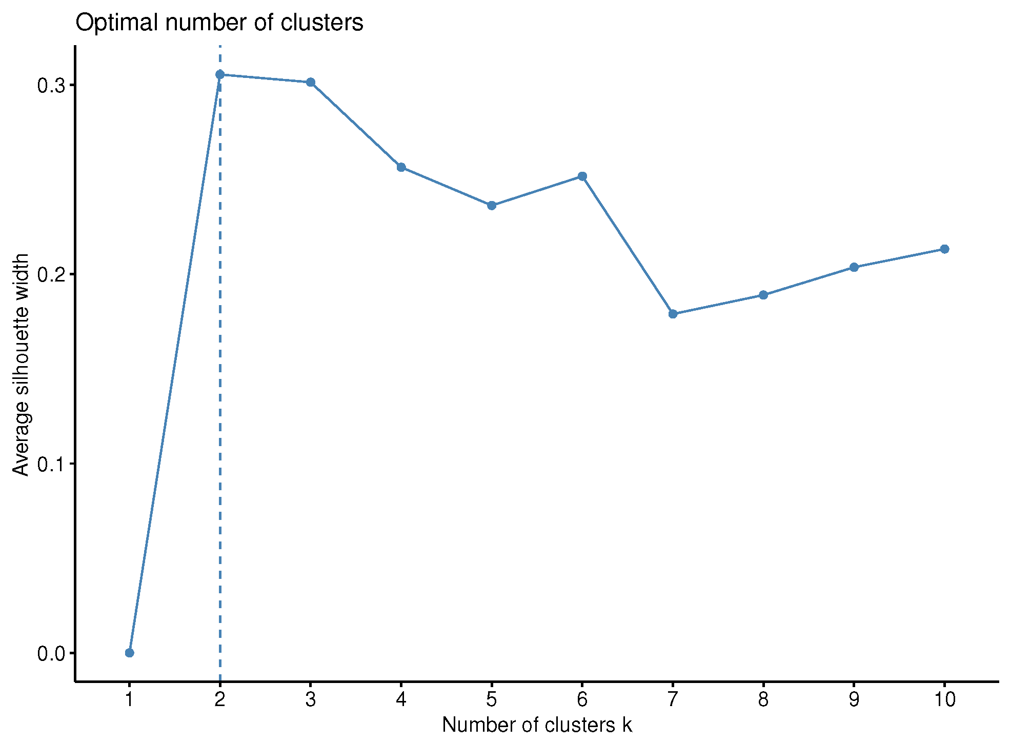
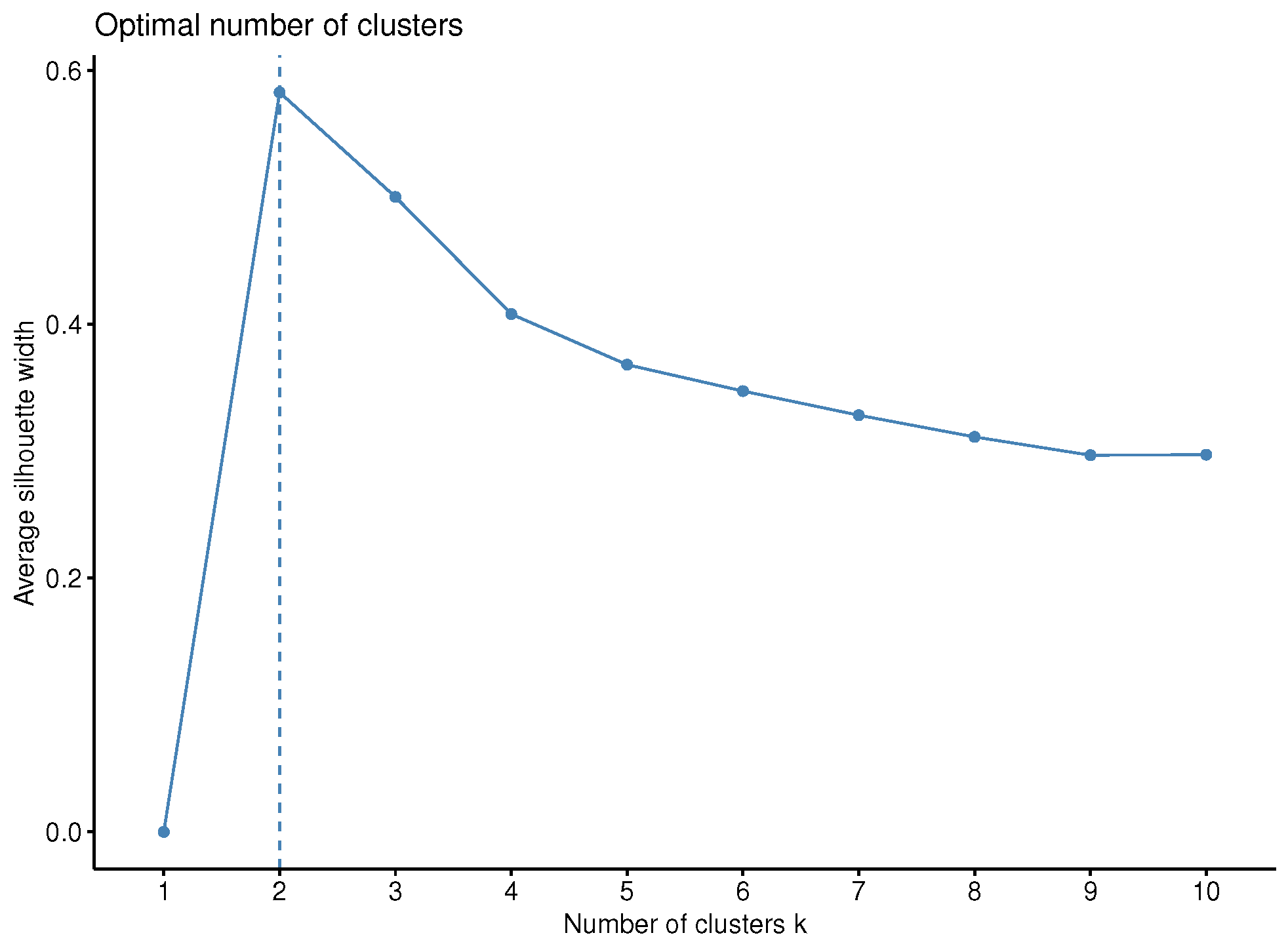
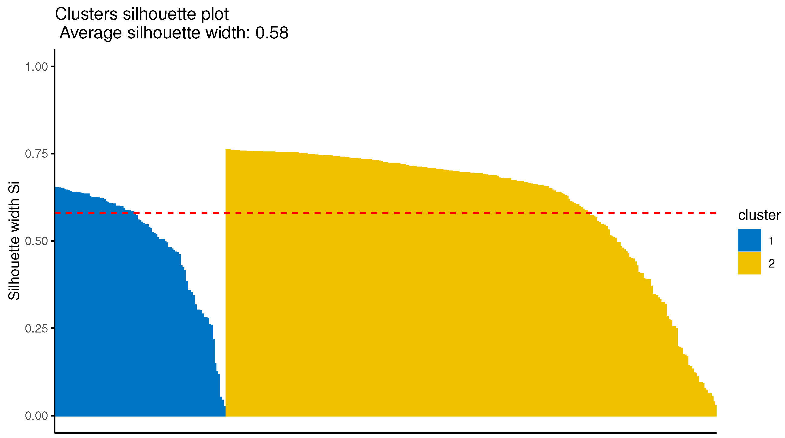
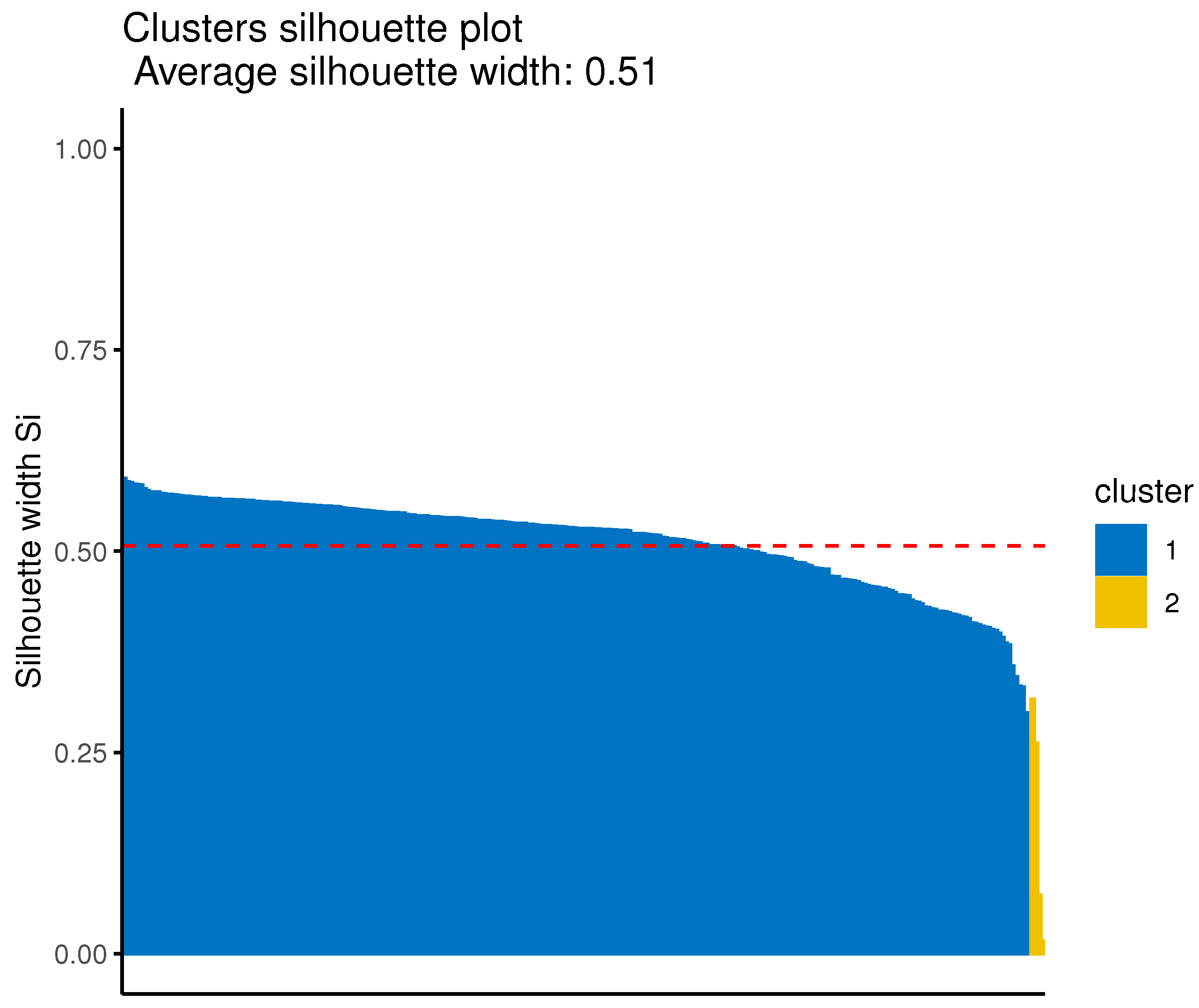
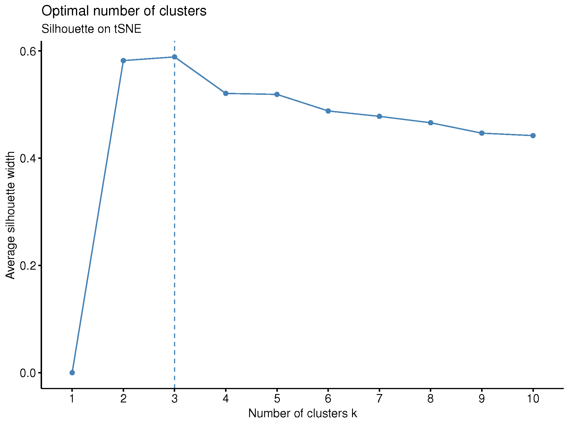
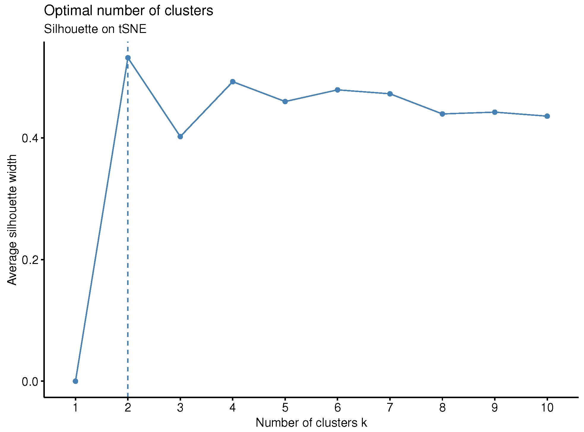
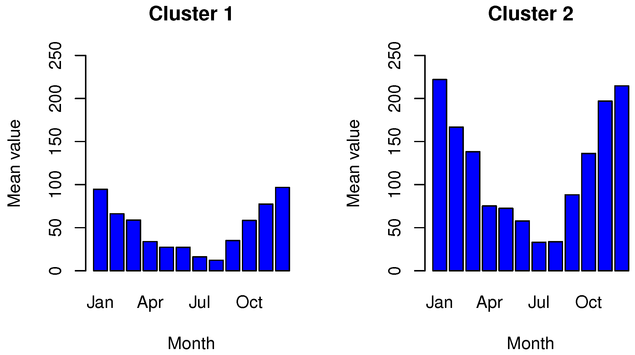
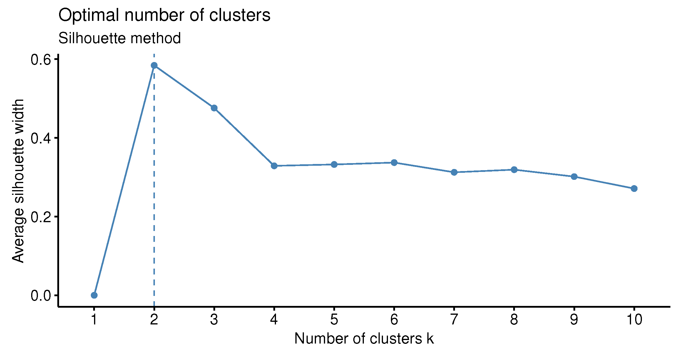
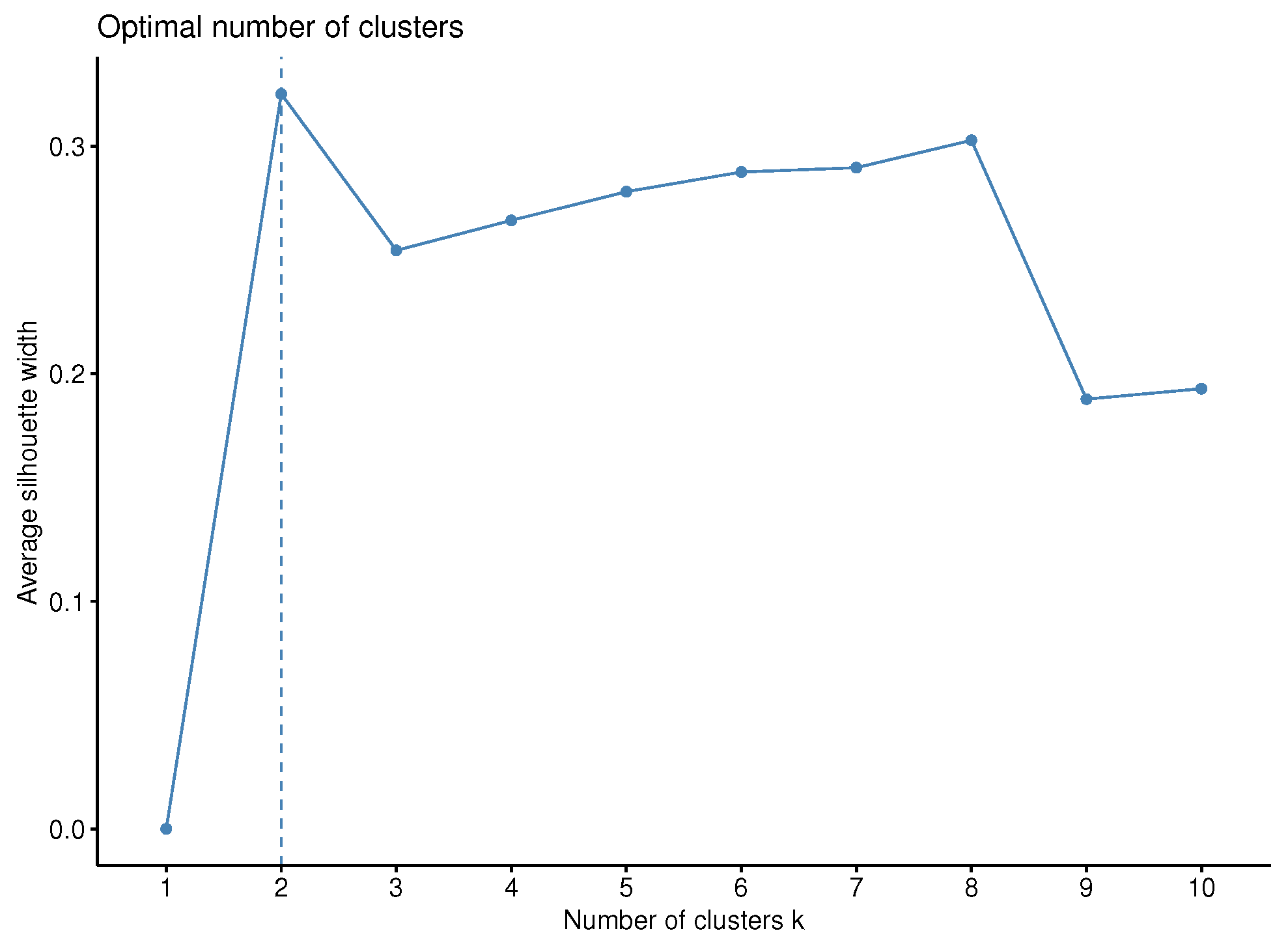
Considering the average silhouette width, the optimal number of clusters is found to be equal to two for both cases (Figure 1 and  Figure 2). The Davies–Bouldin index leads to the same optimal number as well. Regarding the first case, i.e., the case of the precipitation data, the first cluster consists of 313 stations. The rest of the stations (57) are assigned to the second cluster. Figure 3 presents the mean seasonal indices for these two clusters under the initial case concerning the precipitation. From the figure, it is clear that the first cluster consists of areas of lower rainfall in all months. For further insights on the clusters, the boxplots of the monthly seasonal indices are presented in Figure 4.

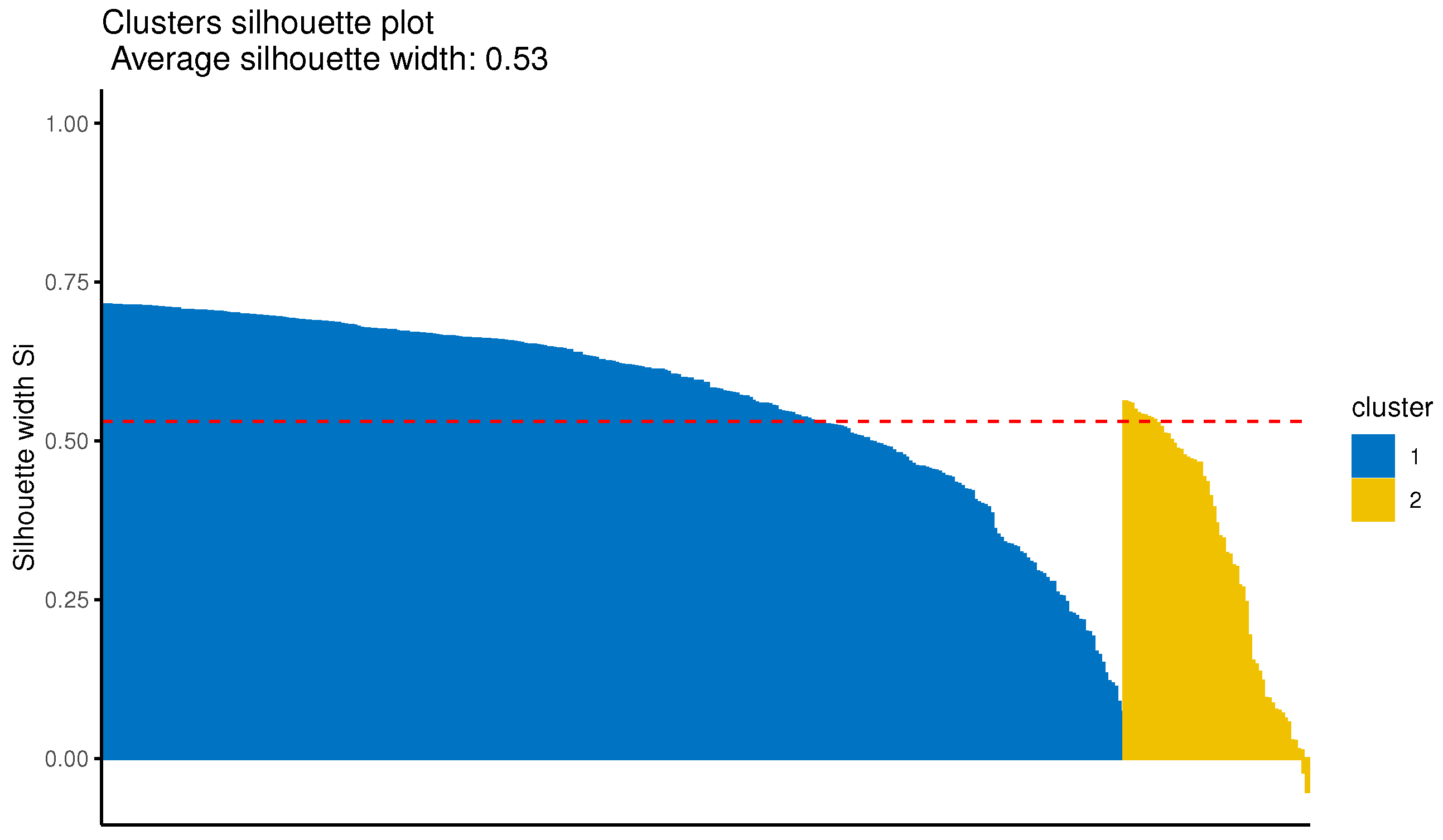
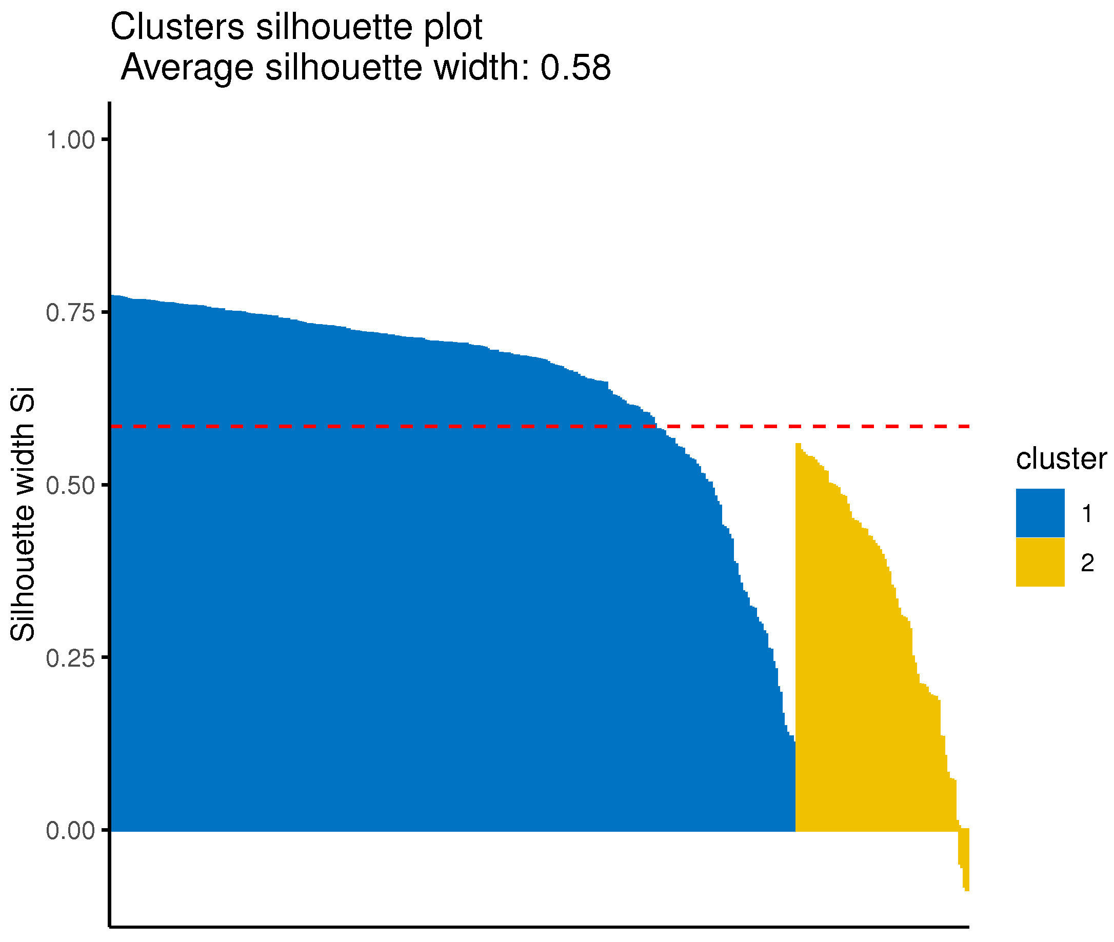
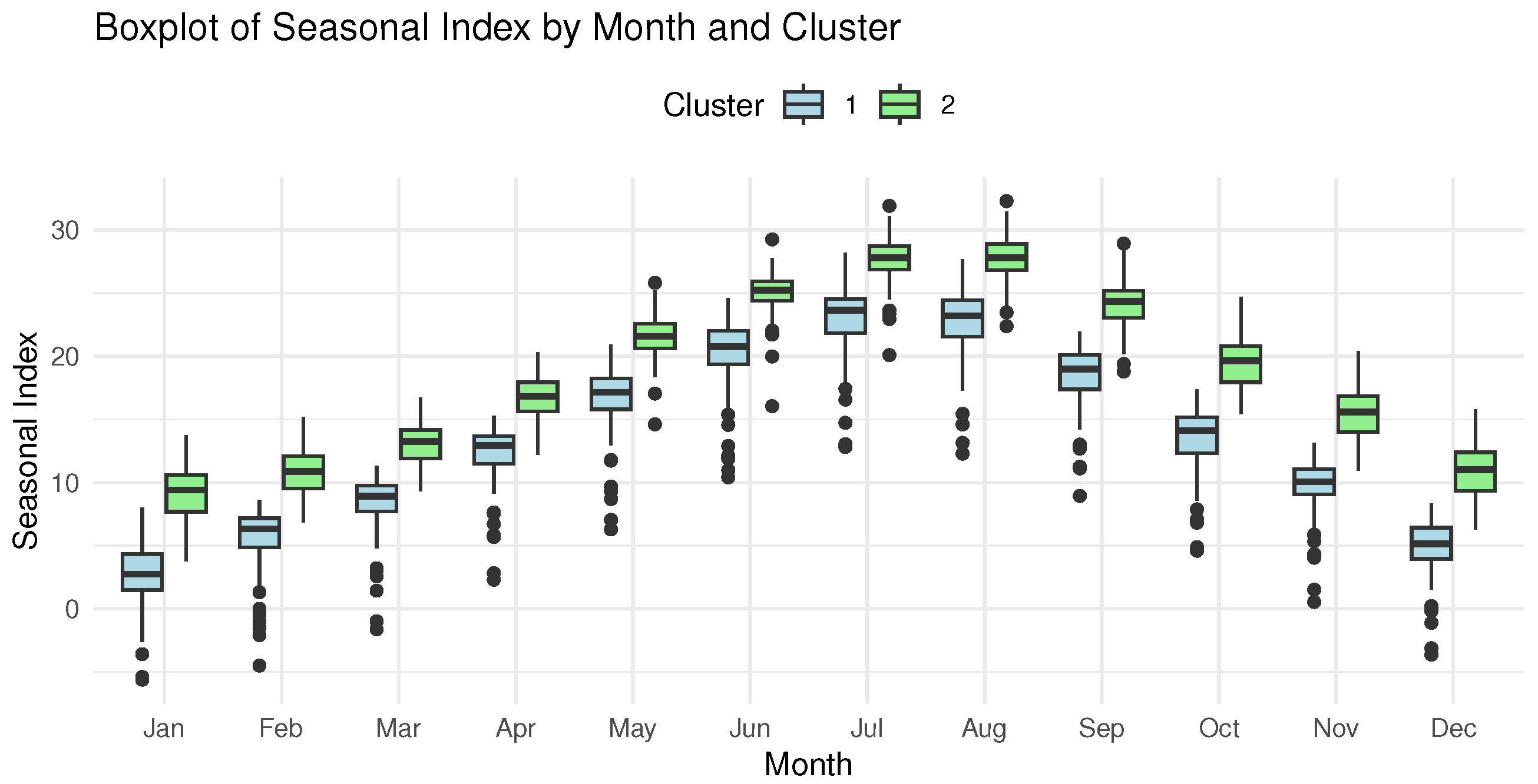
The first cluster of the case with the mean temperature data consists of 96 stations, while the second consists of 274 stations. In Figure 5, the corresponding mean seasonal indices for these two groups are presented concerning the second case of the mean temperature, while in Figure 6, the boxplots of the monthly seasonal indices are depicted. In addition, for both cases, plots of average silhouette width per cluster for this level of clustering are provided in the Appendix C.2.

The first level of clustering, using both meteorological features, identifies two climatic regions determined by orography and the passage of depressions from the west, i.e., the Pindos mountain range, extending from the NW edge to the Crete island, dividing the country into two major hydroclimatic areas, the water-rich one and the semi-arid eastern ones [82]. More specifically, cluster 1 based on precipitation includes stations of medium to low precipitation rates in Eastern and Southern Greece with mean annual precipitation between 219.16 and 861.29 mm and a mean altitude of 126.52 m above sea level. On the other hand, cluster 2 includes stations of high to very high precipitation rates in Northern Greece with a mean annual precipitation between 924.42 and 2494.14 mm and a mean altitude of 741.14 m above sea level. It is worth mentioning that 84.59% of all stations are included in the “dry” cluster 1, while the remaining 15.4% of the stations are embodied within the “wet” cluster 2.

It is of note that, while these clusters align more or less geographically with the Pindos mountain range, this division emerges solely from the temporal patterns of the data, such as contrasting winter precipitation peaks (see for example the 3rd subgroup with 181.33 mm in November vs. the 1st subgroup with 75.48 mm). Spatial attributes (e.g., elevation or proximity) are not inputs to the algorithm.

Cluster 2, based on temperature, includes circa 74% of stations with high mean annual temperature (18.5 °C), ranging between 15.84 °C and 22.25 °C and a mean altitude of 144 m above sea level. On the other hand, cluster 1 includes stations of low mean annual temperature (13.1 °C) ranging between 3.84 °C and 15.77 °C and a mean altitude of 759.1 m above sea level, located mainly in mountainous areas.

4.2.2. Second-Level Clustering

Regarding the second-level clustering, the missing values for each time series are imputed by splitting the time series into seasons and afterwards, performing interpolation to deal with the missing values separately for each of the resulting time series datasets. The percentage of missing values for precipitation and mean temperature ranges from 0 to 85% with a mean of 45% across the different available stations. The time series in-cluster dissimilarity matrices are afterwards computed (based on the Dynamic Time Warping method computed for each pair of objects) for each cluster, determined by the first-level clustering. Using hierarchical cluster analysis, each cluster is split into sub-clusters. The optimal number of clusters is determined again by the silhouette method.

Each first-level cluster is again split into two sub-clusters (see Appendix C.1). More specifically, in the case of precipitation, the stations of the second main cluster are split into 50 and 7 stations, while the stations of the first main cluster are divided into 291 and 22. Stations under the second scenario and the first main cluster are split into 90 and 6 stations, and those stations that result in the second main cluster are divided into clusters comprised of 270 and 4 stations. Indicatively, for this level of clustering and for the second case, plots of the average silhouette width per cluster are provided in the Appendix C.2.

A rain gauge only provides the depth of rain at the point where the station is located, so rain on an area should be estimated from that point of measurement, using surface integration methods. In this study, the Thiessen polygons method [83], using ArcGIS Pro 2.5, is applied to divide the study area into regions (polygons) where every point within a given polygon is closer to its associated data point than to any other. Given the set of weather stations, Thiessen polygons delineate the area most likely influenced by each station. This method is still popular and widely applied because of its high calculation accuracy, fast computation, and simplicity, requiring only the area data of sample points to estimate average rainfall (and other hydrometeorological factors, e.g., solar radiation) over a bounded area [84,85].

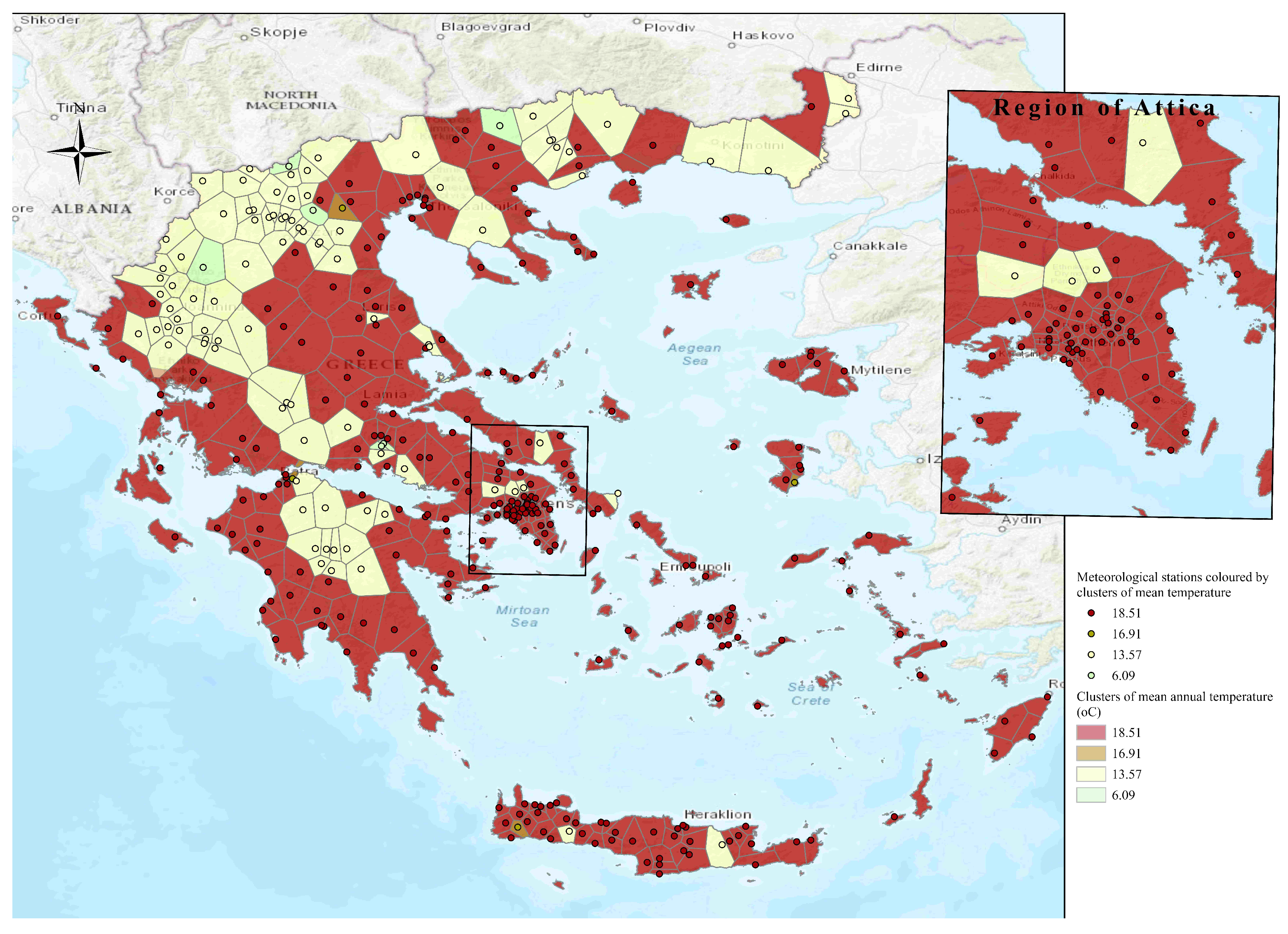
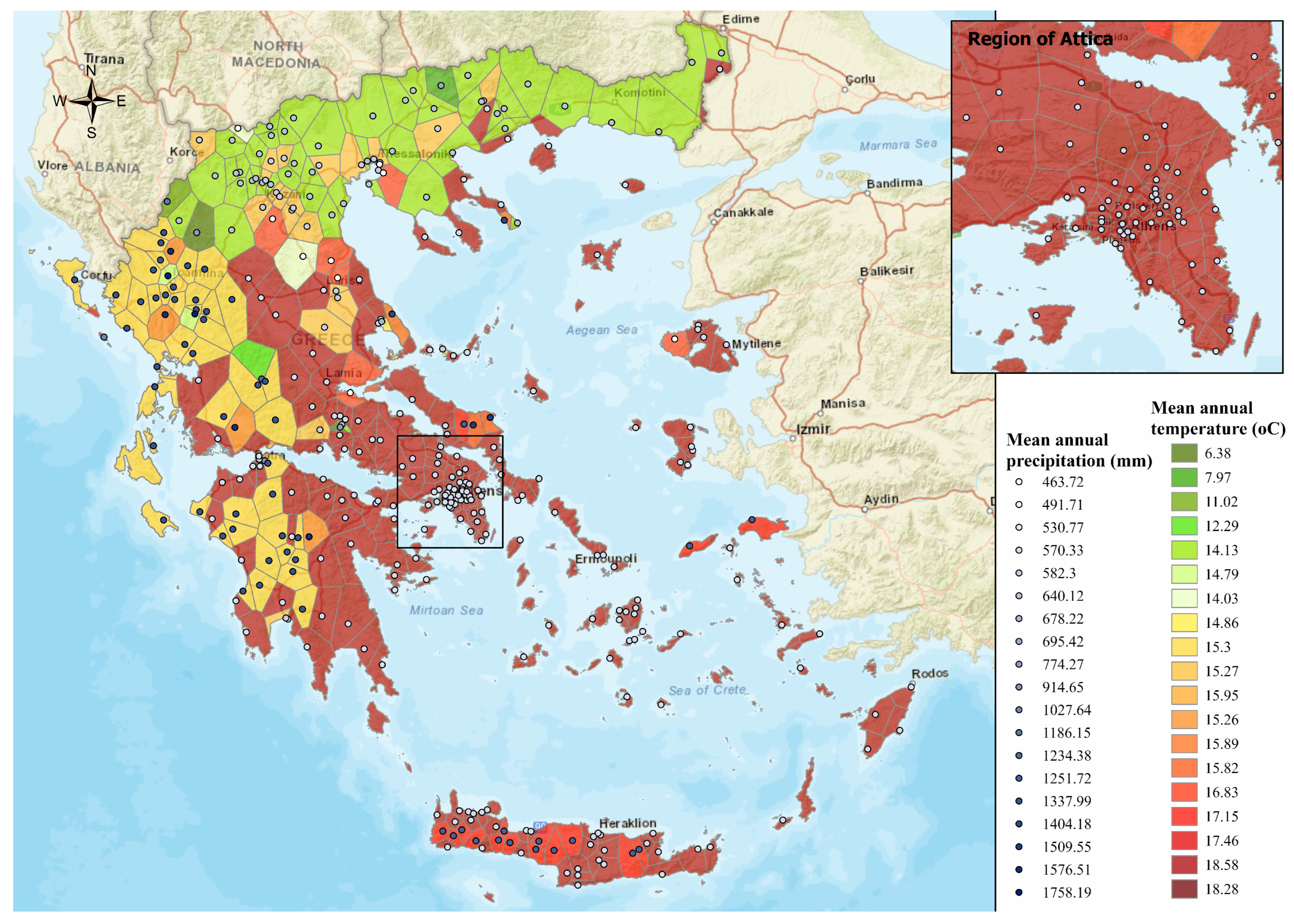
In Figure 7 are depicted the four sub-clusters regions (using Thiessen polygons) for the precipitation time series, and in Figure 8, the four sub-clusters regions for the mean temperature time series. The second level clustering divides each of the above-mentioned groups into two subgroups, resulting in four final groups of similar mean annual precipitation rates. More precisely, the previous “dry” cluster 1 includes almost the entire of Eastern Greece and most of the coastal and low-altitude regions of Western Greece. It is split into (a) a “very dry” cluster (including 92.97% of the stations of the first cluster) with mean annual precipitation of 589.68 mm, including among others the Region of Attica (the most densely populated metropolitan region of Athens) as well as Thessaloniki, the second biggest city of Greece, and (b) a “less dry” cluster (including 7.03% of the stations) with mean annual precipitation 792.65 mm including regions located in Crete, some islands in Aegean sea (e.g., Chios, Ikaria, Lesvos, Thassos, Rhodos, and Kastelorizo), and a few regions in the continental Greece (e.g., Kalamata in Messinia, Geraki in Lakonia, and Tatoi in Attica). Similarly, the previous “wet” cluster with mainly mountainous areas is divided into (a) a “wet” cluster, including 87.72% of the stations, with mean annual precipitation 1342.27 mm with regions in Western Greece around the mountainous systems extending from North to South, (Pindus, Panachaiko, Erymanthos, Chelmos, Taygetos, etc.), and (b) a “very wet” cluster, including the rest 12.28% of the stations, with mean annual precipitation 2099.75 mm, including the most rainy areas (>1845 mm) in Northern Greece, located in Epirus (i.e, Ioannina, Thesprotia, and Arta) and a small area of Evrytania.

Further, the second-level clustering divides each of the above-mentioned groups into two subgroups, resulting in four final groups of similar mean annual temperature. More precisely, the previous “warm” cluster 2 is further split into (a) a “very warm” cluster (including 72.97% of all the stations in total) with mean annual temperature 18.51 °C including most of Eastern Greece, all islands and a wide coastal area of Western Greece and (b) a “ less warm” cluster (including 1.08% of all the available stations) with mean annual temperature 16.91 °C, including only four stations in Achaia, Chania, Chios, and Veroia. Similarly, the previous “cold” cluster is divided into (a) a “cold” cluster, including 24.32% of the stations, with mean annual temperature 13.57 °C with most regions located in Northern Greece (e.g., Alexandroupoli, Ioannina, and Metsovo) and at the mountainous (e.g., Panachaiko) and (b) a “very cold” cluster, including the rest 1.62% of the stations, with mean annual temperature 6.09 °C with altitude >1500 (e.g., Kaimaktsalan and Parnassos). The above-mentioned insights, for both scenarios, are summarized for comparison purposes in

Table 2. Summarized results of the four identified sub-cluster regions under the 2nd scenario (i.e., precipitation-based clusters).

Cluster	Sub-Cluster	Percentage of Stations	Mean Annual Precipitation	Notable Regions
Dry (Cluster 1)	Very Dry	92.97%	589.68 mm	Eastern Greece, Attica (Athens), Thessaloniki.
	Less Dry	7.03%	792.65 mm	Crete, Aegean islands (Chios, Ikaria, Lesvos, etc.), Continental Greece (e.g., Kalamata, Geraki, and Tatoi).
Wet (Cluster 2)	Wet	87.72%	1342.27 mm	Mountainous areas in Western Greece (Pindus, Panachaiko, Erymanthos, etc.).
	Very Wet	12.28%	2099.75 mm	Rainy areas in Northern Greece, located in Epirus (Ioannina, Thesprotia, and Arta), Evrytania.

 and 

Table 3. Summarized results of the four identified sub-cluster regions under the 2nd scenario (i.e., temperature-based clusters).

Cluster	Sub-Cluster	Percentage of Stations	Mean Annual Temperature	Notable Regions
Warm (Cluster 3)	Very Warm	72.97%	18.51 °C	Eastern Greece, islands, coastal Western Greece.
	Less Warm	1.08%	16.91 °C	Four stations: Achaia, Chania, Chios, and Veroia.
Cold (Cluster 4)	Cold	24.32%	13.57 °C	Northern Greece (e.g., Alexandroupoli, Ioannina, and Metsovo), mountainous areas.
	Very Cold	1.62%	6.09 °C	High-altitude areas (>1500 m), e.g., Kaimaktsalan and Parnassos.

, whereas in

Table 4. Descriptive statistics for the four identified sub-cluster regions for precipitation time series.

	Month	Mean	SD	Median	Min	Max		Month	Mean	SD	Median	Min	Max
1st subgroup (members: 291)	Jan	88.83	40.45	76.90	27.93	245.78	3rd subgroup (members: 50)	Jan	204.74	69.48	201.76	63.60	386.90
	Feb	63.16	29.93	59.07	6.07	161.13		Feb	154.11	71.23	141.43	40.05	449.70
	Mar	57.66	19.68	53.47	23.25	123.80		Mar	130.75	38.37	120.16	61.45	241.55
	Apr	33.69	13.91	32.65	3.60	69.88		Apr	71.40	20.61	68.36	37.37	115.33
	May	27.74	17.65	24.09	0.30	84.11		May	66.51	26.13	61.79	20.75	118.63
	Jun	28.20	20.03	25.76	0.27	120.95		Jun	53.94	22.20	55.10	12.20	121.46
	Jul	16.89	15.81	11.22	0.00	78.63		Jul	31.49	15.74	32.58	2.07	70.49
	Aug	12.64	13.66	7.40	0.00	69.25		Aug	32.43	14.71	33.19	4.91	65.00
	Sep	35.67	21.51	33.20	0.00	106.81		Sep	85.91	29.94	85.72	28.40	196.55
	Oct	58.01	26.40	53.40	12.60	157.04		Oct	129.35	36.52	126.80	67.60	243.12
	Nov	75.48	33.37	69.13	20.40	197.53		Nov	181.33	55.01	180.17	71.55	367.08
	Dec	91.71	36.61	83.70	28.60	229.17		Dec	200.31	74.55	182.61	80.60	463.56
2nd subgroup (members: 22)	Jan	170.82	59.60	161.93	77.97	329.20	4th subgroup (members: 7)	Jan	345.18	34.17	340.54	284.87	398.42
	Feb	106.19	49.83	96.81	41.13	205.77		Feb	257.64	42.62	271.20	201.77	325.23
	Mar	74.25	26.08	75.19	38.13	122.10		Mar	191.30	26.80	188.18	155.60	238.28
	Apr	36.09	20.73	31.80	14.30	111.80		Apr	102.92	30.83	109.49	60.83	142.87
	May	21.53	11.27	19.66	0.80	48.94		May	114.97	12.10	112.74	99.08	136.52
	Jun	14.66	13.66	7.64	0.33	52.49		Jun	85.68	15.07	82.90	69.80	112.20
	Jul	5.26	5.80	3.96	0.00	21.00		Jul	44.00	8.94	48.00	29.78	53.70
	Aug	7.12	10.47	3.52	0.00	46.90		Aug	42.93	11.62	39.57	33.11	68.24
	Sep	26.51	16.48	25.00	1.60	64.62		Sep	104.67	36.86	101.16	48.00	158.03
	Oct	62.94	28.11	62.02	20.92	120.43		Oct	185.18	39.01	186.81	137.13	241.15
	Nov	103.35	34.30	98.22	47.90	181.53		Nov	308.28	41.57	319.92	241.09	355.34
	Dec	163.93	48.01	154.75	82.71	255.93		Dec	317.00	72.24	295.86	234.58	429.80

 and 

Table 5. Descriptive statistics for the four identified sub-cluster regions for mean temperature time series.

	Month	Mean	SD	Median	Min	Max		Month	Mean	SD	Median	Min	Max
1st subgroup (members: 90)	Jan	2.90	1.86	2.95	−1.57	8.00	3rd subgroup (members: 270)	Jan	9.19	2.19	9.42	3.75	13.74
	Feb	5.97	1.72	6.45	1.30	8.61		Feb	10.86	1.74	10.89	6.82	15.16
	Mar	8.78	1.55	8.95	3.21	11.32		Mar	13.03	1.50	13.28	9.30	16.74
	Apr	12.70	1.62	13.04	6.71	15.28		Apr	16.77	1.45	16.81	12.19	20.31
	May	17.00	1.93	17.24	9.67	20.92		May	21.59	1.36	21.57	18.33	25.80
	Jun	20.73	2.12	20.85	11.88	24.58		Jun	25.10	1.40	25.21	16.04	29.24
	Jul	23.47	1.90	23.73	18.58	28.16		Jul	27.76	1.45	27.81	20.08	31.89
	Aug	23.19	1.94	23.31	18.49	27.69		Aug	27.81	1.50	27.80	23.74	32.27
	Sep	18.87	1.85	19.15	12.86	21.91		Sep	24.16	1.51	24.36	19.38	28.91
	Oct	13.98	1.72	14.17	8.81	17.37		Oct	19.45	1.86	19.65	15.42	24.68
	Nov	10.02	1.44	10.24	5.86	13.14		Nov	15.39	1.97	15.62	10.93	20.38
	Dec	5.21	1.57	5.33	1.53	8.31		Dec	10.97	2.08	11.02	6.30	15.76
2nd subgroup (members: 6)	Jan	−3.63	1.54	−3.10	−5.61	−2.07	4th subgroup (members: 4)	Jan	7.62	1.99	8.08	4.80	9.49
	Feb	−1.60	1.60	−1.25	−4.50	−0.01		Feb	9.98	0.73	10.10	8.98	10.74
	Mar	0.97	1.88	1.43	−1.64	3.01		Mar	12.07	0.98	12.08	10.86	13.26
	Apr	5.30	2.28	5.75	2.30	7.62		Apr	16.04	1.15	15.95	14.73	17.52
	May	9.13	2.30	9.00	6.28	11.77		May	18.83	3.65	19.17	14.60	22.38
	Jun	12.73	1.99	12.50	10.40	15.48		Jun	24.20	1.61	24.41	22.27	25.68
	Jul	15.41	2.22	15.63	12.80	17.94		Jul	24.70	2.06	24.47	22.93	26.91
	Aug	15.17	2.34	15.01	12.28	18.34		Aug	24.50	1.96	24.45	22.37	26.73
	Sep	10.98	1.76	11.17	8.92	13.00		Sep	22.03	2.57	22.21	18.77	24.94
	Oct	6.64	1.60	6.95	4.59	8.57		Oct	18.45	1.68	18.65	16.21	20.29
	Nov	3.32	1.86	4.11	0.54	5.34		Nov	14.61	1.99	14.57	12.22	17.06
	Dec	−1.30	1.69	−0.65	−3.63	0.21		Dec	9.63	1.78	9.49	7.60	11.95

, some descriptive statistics for all four regions are identified through second-level clustering. This stage further divides each of the two initial clusters into two sub-clusters, resulting in four distinct groups per scenario, clearly highlighting the unique characteristics of each cluster.

4.3. Multivariate Case

The available information on the exact meteorological stations that were employed in the previous section is once again employed. This time, however, the precipitation and mean temperature levels were considered simultaneously.

4.3.1. First-Level Clustering

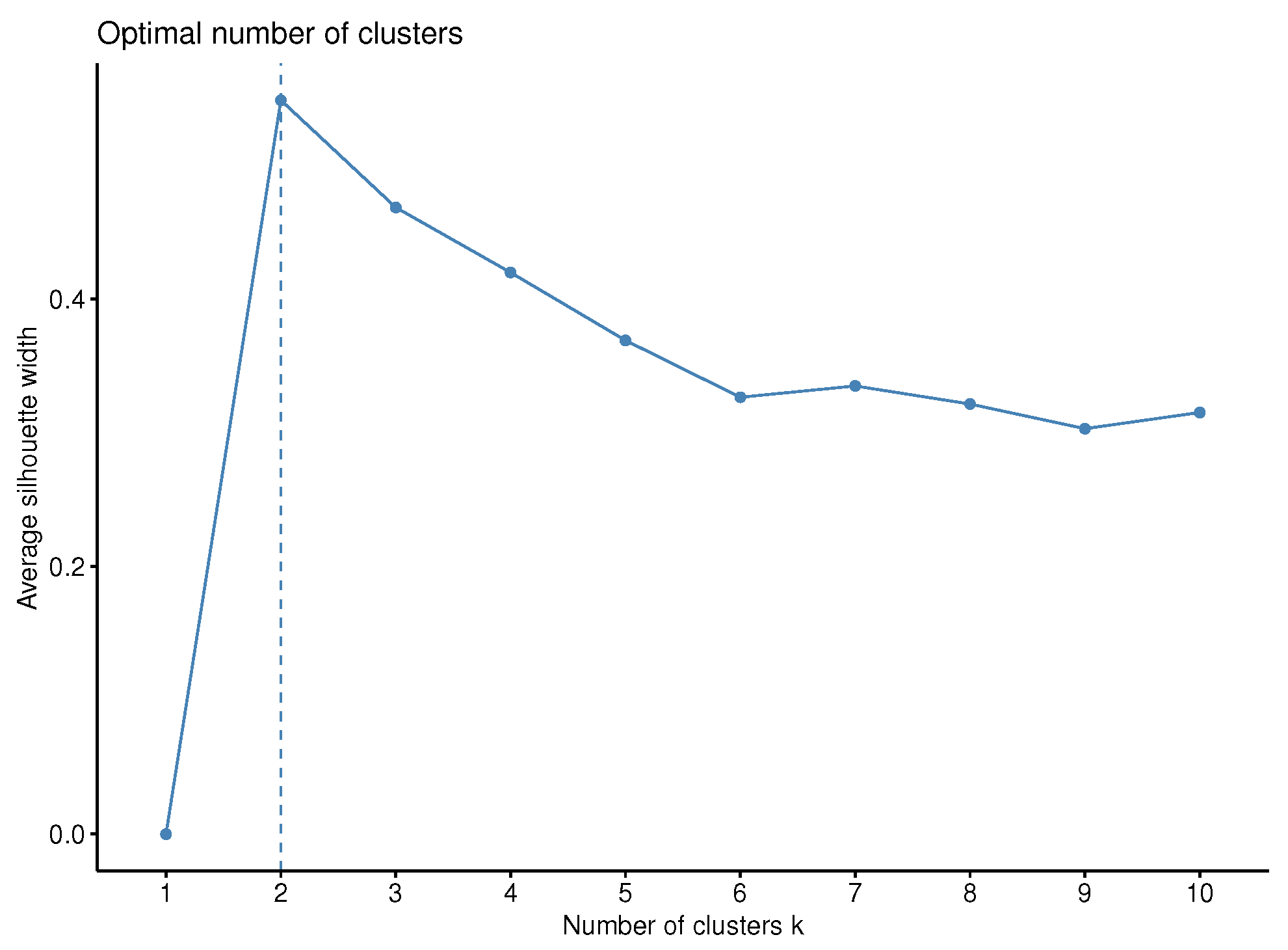
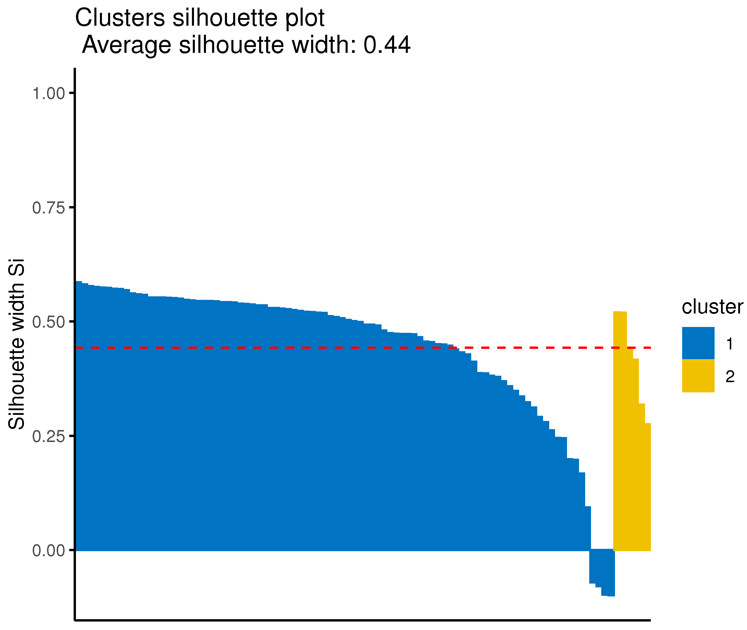
Following the procedure described in Section 3, for the first level of clustering, seasonal indices of both precipitation levels and mean temperatures are calculated. As for the second step, multidimensional scaling is employed in these seasonal indices, with the aid of the distance matrix given by relation (9). After executing the K-means algorithm and computing also the Davies–Bouldin index, the optimal number of clusters is revealed, and it is equal to two clusters (Figure 9). More precisely, the first cluster contains 296 stations, while the second consists of 74 stations. In Figure 10, the mean seasonal indices are presented for both characteristics for these two clusters. The upper plots concern the mean precipitation levels, while those below take into consideration the mean of the average temperature levels. As an illustrative example, a plot of the average silhouette width per cluster corresponding to this clustering level is provided in the Appendix C.2.

Generally, the first-level clustering identifies two climatic regions, mainly determined by the great mountain chains along the central part extending from the north to the south and other mountainous bodies. The two groups embody, on one side, the dry Eastern Greece, including also the dry metropolitan area of Athens (the Attica Region, hosting more than half of the Greek population), and, on the other side, the wet Northern and Western Greece.

4.3.2. Second-Level Clustering

In accordance with the procedure mentioned in the previous section, the “Seasonally Splitted Missing Value Imputation” method is performed in order to impute missing values in both cases of raw time series. That is, the time series concerning the precipitation levels as well as the time series concerning the mean temperatures on each of the available meteorological stations. The resulting time series objects are afterwards grouped based on the resulting clusters from the first level of clustering. In order to proceed to the second level of the clustering (i.e., hierarchical clustering), Euclidean timed and spaced distance is calculated.

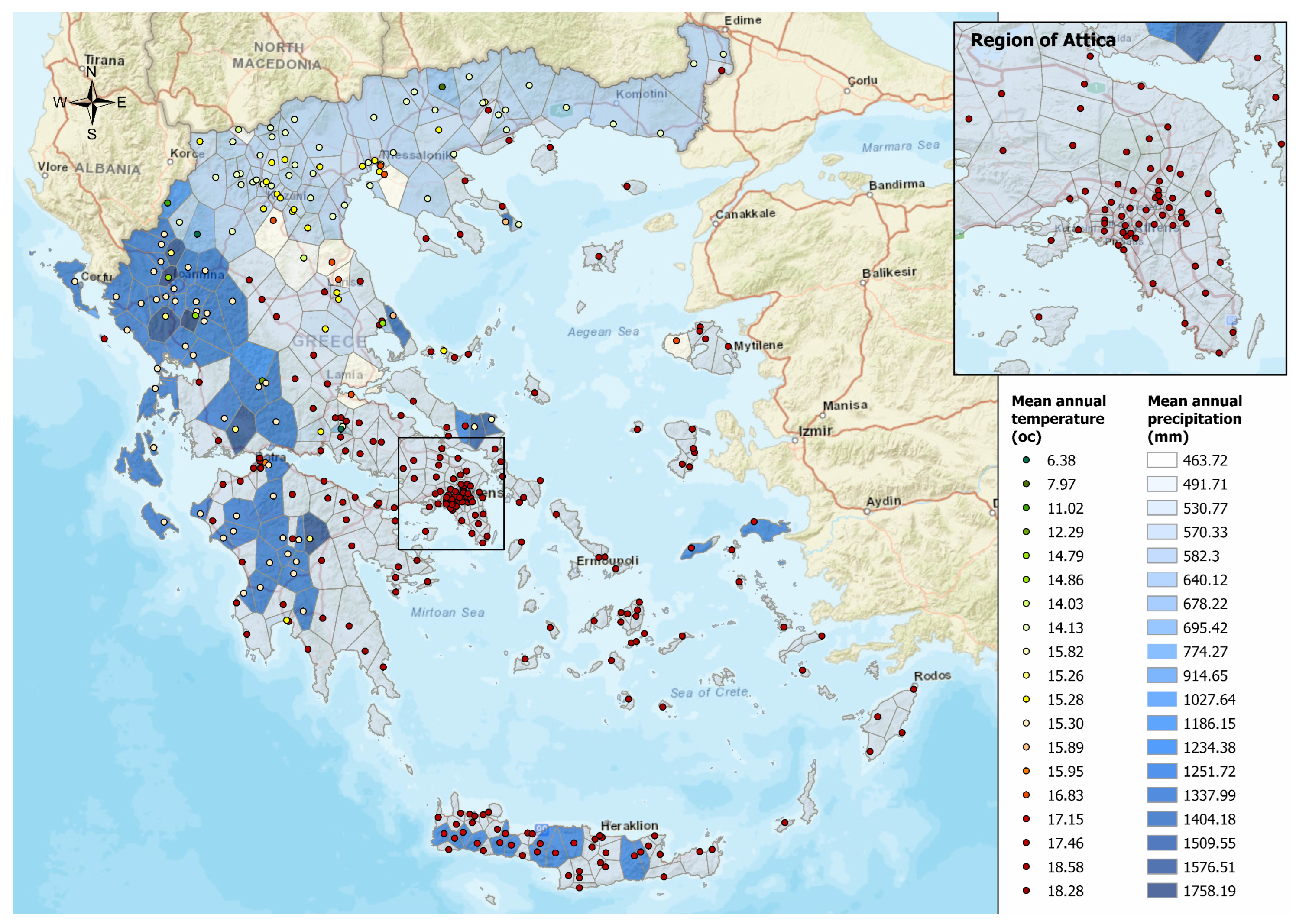
The average silhouette width criterion revealed that the optimal number of sub-clusters is 9 for the resulting first cluster of the first level clustering and 10 for the second cluster, respectively. Due to the total count of the sub-clusters, the tables with the descriptive statistics are omitted but are available in the Appendix C.1. In Figure 11 and Figure 12 the resulting sub-clusters are depicted.

The second-level clustering identifies nineteen sub-clusters driven by multivariate temporal patterns (e.g., synchronized precipitation–temperature cycles). These clusters are in compliance with the great spatial weather variety of the country. Situated at the southern end of the Balkan Peninsula, Greece presents a complex and fragmented topography with a strong relief resulting in a high geomorphological diversity [86]. More precisely, the western side of the country is mainly mountainous, including only a few plains. The eastern side of the mainland presents a contrary topography with many plains displaying relief near the coastline. This complex topography, both horizontal (long coastline and many islands) as well as vertical (many mountain ranges and individual mountains up to 2904 m), contributes to the creation of a mosaic of climates in the country. While this results in the well-known spatial weather diversity in Greece, the identified sub-clusters reflect temporal coherence, not spatial intuition. For example, high-altitude stations in Crete (south) are grouped with northern mountainous areas due to shared winter rainfall spikes, despite geographical differentiation.

Moving upwards from sub-cluster 1 to sub-cluster 9 (of the ‘drier’ cluster 1), generally, the mean annual precipitation increases, and the mean annual temperature decreases. The same holds for sub-clusters 10–19 of the second main cluster. Nevertheless, some sub-clusters present a much more complex pattern, including stations with a combination of high precipitation (considering the rest of sub-clusters 1–9) with a low temperature (e.g., sub-cluster 5) or the opposite (e.g., cluster 11). The regions of cluster 1 have 570.33 mm mean annual precipitation and 18.58 °C. The regions of sub-clusters 2 and 3 have progressively higher mean annual precipitation rates, i.e., 582.3 mm and 640.12 mm, and lower temperatures, i.e., 15.27 °C and 14.13 °C, respectively. The regions of sub-cluster 4 have a lower mean annual precipitation height (463.72 mm) combined with a higher mean annual temperature of 16.83 °C. On the contrary, the regions of cluster 5 have a significantly higher mean annual precipitation (774.27 mm) and a much lower mean annual temperature of 6.37 °C. The regions of cluster 6 follow the general pattern with 491.71 mm mean annual precipitation and 16.83 °C. Cluster 7 is characterized by a combination of moderate mean annual precipitation (695.42 mm) with a very low mean annual temperature (6.37 °C). In this cluster, the algorithm includes only one station (1515 mm altitude) at the Lailias mountains, situated in the north of Greece, belonging to the mountain range of Eastern Macedonia.

The next clusters follow the general pattern of increasing precipitation and variable temperature, with some exceptions as well, in compliance with the complex morphology of Greece. In

Table 6. Summary of sub-clusters for clusters 1 and 2.

Cluster	Sub-Cluster	Mean Annual Precipitation	Mean Annual Temperature
1	1	570.33 mm	18.58 °C
	2	582.3 mm	15.27 °C
	3	640.12 mm	14.13 °C
	4	463.72 mm	16.82 °C
	5	774.27 mm	6.38 °C
	6	491.71 mm	14.03 °C
	7	695.42 mm	7.97 °C
	8	678.22 mm	14.85 °C
	9	530.77 mm	18.28 °C
2	10	1337.99 mm	15.3 °C
	11	1251.72 mm	17.15 °C
	12	1576.51 mm	15.26 °C
	13	1758.19 mm	14.79 °C
	14	1404.18 mm	15.89 °C
	15	1234.38 mm	12.29 °C
	16	914.65 mm	15.95 °C
	17	1509.55 mm	15.82 °C
	18	1027.64 mm	17.46 °C
	19	1186.15 mm	11.02 °C

, the mean annual precipitation along with the mean annual temperature for each of the sub-clusters are presented. Sub-cluster 19 includes only one station (1240 mm altitude) at Plikati, Ioannina in Western Greece. Sub-cluster 12 represents regions with very high annual precipitation heights (1758 mm). It includes mainly regions of Midwestern Greece. A few regions from Eastern Greece with high precipitation rates (which have been identified also by the National Observatory of Athens in the annual lists of meteorological stations with the highest rainfall rates) are also included in sub-clusters 11, 14, and 17. Characteristic examples are Setta in Evoia and Zagora in Pilio, the last one having experienced devastating flooding following extreme rainfall associated with storm Daniel [87].

Overall, the 19 identified distinct sub-clusters based entirely on temporal patterns in precipitation and temperature, as depicted in Figure 11 and Figure 12, are in accordance with the very rare previous studies (e.g., [86]) with respect to the different time periods, scope of the studies, and methodological procedures.

5. Conclusions

Considering the first case of univariate time series, meaning the case of precipitation time series, the proposed method identified four regions with similar precipitation characteristics and patterns in Greece. These clusters could result from the division of Greece by the Pindos Mountain range, where regions located along the mountain passage (i.e., the most mountainous) receive higher precipitation levels. A similar result was derived from the mean temperature time series, where once again, four regions of Greece were identified as having similar mean temperatures. Regions with higher mean altitudes consistently maintained lower temperatures compared to those at lower altitudes or near the sea.

In the multivariate scenario, the proposed method identified 19 distinct sub-clusters based entirely on temporal patterns in precipitation and temperature. While some clusters align with known geographical features (e.g., the Pindos mountain range), their formation was strictly data driven through seasonal indices and DTW-aligned raw series, prioritizing temporal patterns over spatial intuition. This approach proved particularly effective in Greece’s complex topography, where proximate areas often exhibit markedly different meteorological behaviors. The method revealed meaningful, data-driven subgroups that transcend geography (e.g., high-altitude stations in Crete clustering with northern mountainous areas), demonstrating that temporal patterns can capture climatic relationships that spatial correlations alone might miss. While spatial information could enhance interpretability in some contexts, our results show that temporal features can effectively reveal Greece’s diverse climatic regions.

Finally, it should be taken into consideration that there are parts of Greece where the coverage of automated weather stations is insufficient (e.g., East Peloponnese, and North or Central Greece). For that reason, along with the complexity of topography that controls both temperature and precipitation, any conclusions should be extracted with caution.

The proposed two-level clustering methodology, however, offers both theoretical and practical implications. Theoretically, it contributes to the study of time series clustering by addressing challenges associated with missing data, unequal series lengths, and seasonal structures, particularly in spatiotemporal environmental data. Practically, the framework provides a data-driven approach to identify meteorologically homogeneous regions. This can support national and regional stakeholders—such as environmental agencies, water resource planners, and climate policy advisors—in identifying climate-sensitive zones for more effective infrastructure planning, risk assessment, and resource allocation. Furthermore, the general structure of the methodology ensures that it can be easily applied to other regions or climatic variables, making it a versatile tool for broader geospatial applications under varying environmental contexts.

As in any methodology, limitations exist and are presented with possible suggestions that could also be part of future work. The method assumes a common seasonal time period across all time series, which may not hold true for geographically diverse meteorological stations with varying local climates. For cases where common seasonality does not exist, adaptive seasonal decomposition techniques (e.g., STL or seasonal autoencoder models) could be an alternative. The extensive or non-random missingness of data could lead to implications when imputation is applied in general, distorting original temporal patterns. In this case, however, the original temporal and seasonal patterns are derived from the first-level clustering when no imputation is performed. Model-based or probabilistic imputation techniques, such as Gaussian Process imputation, could be an option.

As already mentioned, the clustering methods in this work were initially selected for their interpretability, computational efficiency, and widespread use in environmental time series clustering, in order to establish a robust baseline for future method comparisons. A point of interest, however, could be a comparison of the known flexible clustering techniques (e.g DBSCAN) or deep learning-based clustering, options that capture complex relationships, with the proposed methodology. Other comparisons could be with the basic approaches of imputation (KNN imputation, pattern DTW matching) or other state-of-the-art methods like GAIN, DTW LSTM, etc. A promising direction for future research is to utilize temporal modeling techniques, such as HMMs or RNNs, that might provide a richer representation of the dynamic evolution of weather patterns. It should be noted that the clustering focus on dominant seasonal patterns was driven by the data’s high proportion of missing values and the prominent seasonal dynamics of the meteorological data. Incorporating clustering based on extreme/recurrent events would add important insights though.

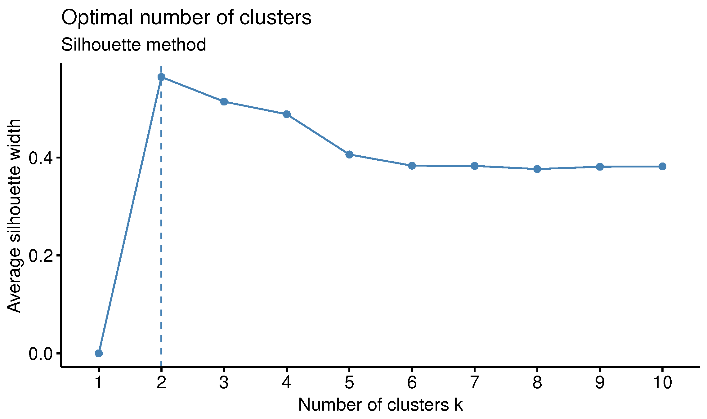
Further, an interesting aspect for future work is to research in the direction of nonlinear dimensionality reduction techniques (e.g., t-SNE and UMAP) to compare the results. Our preliminary applications of t-SNE (see Appendix C) produced clusters inconsistent with the known climatic regions of Greece. This discrepancy is likely due to the sensitivity of these methods to high dimensionality and parameter tuning, and thus is suggested for further study. In addition to the above-mentioned points, it is acknowledged that the present study has been conducted using a meteorological dataset from Greece, and that its generalizability to other geographical regions and climatic conditions has yet to be empirically demonstrated. Nevertheless, the proposed methodology has been developed within a broadly applicable framework, designed to be easily transferable to datasets from other locations. Thus, it is intended to broaden its generalizability to other climatic variables, regions, or climatic zones of global datasets. To enhance usability, an R-Shiny dashboard is planned to be developed in future work, which would allow users to easily explore the clustering results, upload new data, or dynamically view seasonal and spatial patterns.

References

1. Ralanamahatana, C.A.; Lin, J.; Gunopulos, D.; Keogh, E.; Vlachos, M.; Das, G. Mining time series data. In Data Mining and Knowledge Discovery Handbook; Springer: Boston, MA, USA, 2005; pp. 1069–1103. [Google Scholar]
2. Ives, A.R.; Zhu, J. Statistics for correlated data: Phylogenies, space, and time. Ecol. Appl. 2006, 16, 20–32. [Google Scholar] [CrossRef] [PubMed]
3. Liu, Y.; Cizeau, P.; Meyer, M.; Peng, C.K.; Stanley, H.E. Correlations in economic time series. Phys. A Stat. Mech. Its Appl. 1997, 245, 437–440. [Google Scholar] [CrossRef]
4. Lam, C.; Yao, Q.; Bathia, N. Estimation of latent factors for high-dimensional time series. Biometrika 2011, 98, 901–918. [Google Scholar] [CrossRef]
5. Duchon, C.; Hale, R. Time Series Analysis in Meteorology and Climatology: An Introduction; John Wiley & Sons: Hoboken, NJ, USA, 2012. [Google Scholar]
6. Glass, L.; Kaplan, D. Time series analysis of complex dynamics in physiology and medicine. Med. Prog. Through Technol. 1993, 19, 115. [Google Scholar]
7. Tsay, R.S. Analysis of Financial Time Series; John Wiley & Sons: Hoboken, NJ, USA, 2005. [Google Scholar]
8. Touloumi, G.; Atkinson, R.; Tertre, A.L.; Samoli, E.; Schwartz, J.; Schindler, C.; Vonk, J.M.; Rossi, G.; Saez, M.; Rabszenko, D.; et al. Analysis of health outcome time series data in epidemiological studies. Environmetrics 2004, 15, 101–117. [Google Scholar] [CrossRef]
9. Panagoulia, D.; Economou, P.; Caroni, C. Stationary and nonstationary generalized extreme value modelling of extreme precipitation over a mountainous area under climate change. Environmetrics 2014, 25, 29–43. [Google Scholar] [CrossRef]
10. Godsill, S.J.; Doucet, A.; West, M. Monte Carlo smoothing for nonlinear time series. J. Am. Stat. Assoc. 2004, 99, 156–168. [Google Scholar] [CrossRef]
11. Harvey, A.C.; Trimbur, T.M.; Van Dijk, H.K. Trends and cycles in economic time series: A Bayesian approach. J. Econom. 2007, 140, 618–649. [Google Scholar] [CrossRef]
12. Verbesselt, J.; Hyndman, R.; Newnham, G.; Culvenor, D. Detecting trend and seasonal changes in satellite image time series. Remote Sens. Environ. 2010, 114, 106–115. [Google Scholar] [CrossRef]
13. Skarlatos, K.; Bekri, E.S.; Georgakellos, D.; Economou, P.; Bersimis, S. Projecting Annual Rainfall Timeseries Using Machine Learning Techniques. Energies 2023, 16, 1459. [Google Scholar] [CrossRef]
14. Lim, B.; Zohren, S. Time-series forecasting with deep learning: A survey. Philos. Trans. R. Soc. A 2021, 379, 20200209. [Google Scholar] [CrossRef] [PubMed]
15. Gallagher, C.; Lund, R.; Robbins, M. Changepoint detection in climate time series with long-term trends. J. Clim. 2013, 26, 4994–5006. [Google Scholar] [CrossRef]
16. Karioti, V.; Economou, P. Detection of Outlier in Time Series Count Data. In Proceedings of the Advances in Time Series Analysis and Forecasting; Rojas, I., Pomares, H., Valenzuela, O., Eds.; Springer: Cham, Switzerland, 2017; pp. 209–221. [Google Scholar]
17. Maharaj, E.A.; D’Urso, P.; Caiado, J. Time Series Clustering and Classification; CRC Press: Boca Raton, FL, USA, 2019. [Google Scholar]
18. Aghabozorgi, S.; Shirkhorshidi, A.S.; Wah, T.Y. Time-series clustering—A decade review. Inf. Syst. 2015, 53, 16–38. [Google Scholar] [CrossRef]
19. Liao, T.W. Clustering of time series data—A survey. Pattern Recognit. 2005, 38, 1857–1874. [Google Scholar] [CrossRef]
20. Wismüller, A.; Lange, O.; Dersch, D.R.; Leinsinger, G.L.; Hahn, K.; Pütz, B.; Auer, D. Cluster analysis of biomedical image time-series. Int. J. Comput. Vis. 2002, 46, 103–128. [Google Scholar] [CrossRef]
21. Rani, S.; Kautish, S. Association clustering and time series based data mining in continuous data for diabetes prediction. In Proceedings of the 2018 Second International Conference on Intelligent Computing and Control Systems (ICICCS), Madurai, India, 14–15 June 2018; pp. 1209–1214. [Google Scholar]
22. Ernst, J.; Nau, G.J.; Bar-Joseph, Z. Clustering short time series gene expression data. Bioinformatics 2005, 21, i159–i168. [Google Scholar] [CrossRef]
23. Kurbalija, V.; von Bernstorff, C.; Burkhard, H.D.; Nachtwei, J.; Ivanović, M.; Fodor, L. Time-series mining in a psychological domain. In Proceedings of the Fifth Balkan Conference in Informatics, Novi Sad, Serbia, 16–20 September 2012; pp. 58–63. [Google Scholar]
24. Steinbach, M.; Tan, P.N.; Kumar, V.; Klooster, S.; Potter, C. Discovery of climate indices using clustering. In Proceedings of the ninth ACM SIGKDD International Conference on Knowledge Discovery and Data Mining, Washington, DC, USA, 24–27 August 2003; pp. 446–455. [Google Scholar]
25. Bengtsson, T.; Cavanaugh, J.E. State-space discrimination and clustering of atmospheric time series data based on Kullback information measures. Environmetrics 2008, 19, 103–121. [Google Scholar] [CrossRef]
26. Gorji Sefidmazgi, M.; Sayemuzzaman, M.; Homaifar, A.; Jha, M.K.; Liess, S. Trend analysis using non-stationary time series clustering based on the finite element method. Nonlinear Process. Geophys. 2014, 21, 605–615. [Google Scholar] [CrossRef]
27. Han, J.; Pei, J.; Tong, H. Data Mining: Concepts and Techniques; Morgan Kaufmann: Burlington, MA, USA, 2022. [Google Scholar]
28. Rokach, L.; Maimon, O. Clustering methods. In Data Mining and Knowledge Discovery Handbook; Springer: New York, NY, USA, 2005; pp. 321–352. [Google Scholar]
29. Nielsen, F. Hierarchical clustering. In Introduction to HPC with MPI for Data Science; Springer: Cham, Switzerland, 2016; pp. 195–211. [Google Scholar]
30. Kriegel, H.P.; Kröger, P.; Sander, J.; Zimek, A. Density-based clustering. Wiley Interdiscip. Rev. Data Min. Knowl. Discov. 2011, 1, 231–240. [Google Scholar] [CrossRef]
31. Cheng, W.; Wang, W.; Batista, S. Grid-based clustering. In Data Clustering; Chapman and Hall/CRC: Boca Raton, FL, USA, 2018; pp. 128–148. [Google Scholar]
32. Economou, P. A clustering algorithm for overlapping Gaussian mixtures. Res. Stat. 2023, 1, 2242337. [Google Scholar] [CrossRef]
33. McNicholas, P.D. Model-based clustering. J. Classif. 2016, 33, 331–373. [Google Scholar] [CrossRef]
34. Fop, M.; Murphy, T.B. Variable selection methods for model-based clustering. Stat. Surv. 2018, 12, 18–65. [Google Scholar] [CrossRef]
35. Malakar, S.; Goswami, S.; Ganguli, B.; Chakrabarti, A.; Roy, S.S.; Kadhirvel, B.; Rangaraj, A.G. An Lstm Based Adaptive Model for Solar Forecasting Using Clustering. SSRN 2022. Available online: https://ssrn.com/abstract=4028663 (accessed on 24 March 2025). [CrossRef]
36. Sun, H.; Jie, W.; Chen, Y.; Wang, Z. A comparison study of several strategies in multivariate time series clustering based on graph community detection. Appl. Intell. 2025, 55, 530. [Google Scholar] [CrossRef]
37. Yoon, J.; Jordon, J.; Schaar, M. Gain: Missing data imputation using generative adversarial nets. In Proceedings of the International Conference on Machine Learning, Stockholm, Sweden, 10–15 July 2018; pp. 5689–5698. [Google Scholar]
38. Cao, W.; Wang, D.; Li, J.; Zhou, H.; Li, L.; Li, Y. Brits: Bidirectional recurrent imputation for time series. Adv. Neural Inf. Process. Syst. 2018, 31, 6776–6786. [Google Scholar]
39. Paparrizos, J.; Yang, F.; Li, H. Bridging the gap: A decade review of time-series clustering methods. arXiv 2024, arXiv:2412.20582. [Google Scholar]
40. Alqahtani, A.; Ali, M.; Xie, X.; Jones, M.W. Deep time-series clustering: A review. Electronics 2021, 10, 3001. [Google Scholar] [CrossRef]
41. Ienco, D.; Interdonato, R. Deep semi-supervised clustering for multi-variate time-series. Neurocomputing 2023, 516, 36–47. [Google Scholar] [CrossRef]
42. Li, H. Multivariate time series clustering based on common principal component analysis. Neurocomputing 2019, 349, 239–247. [Google Scholar] [CrossRef]
43. Jorge, M.B.; Rubén, C. Time series clustering with random convolutional kernels. Data Min. Knowl. Discov. 2024, 38, 1862–1888. [Google Scholar] [CrossRef]
44. Wang, J.; Du, W.; Yang, Y.; Qian, L.; Cao, W.; Zhang, K.; Wang, W.; Liang, Y.; Wen, Q. Deep learning for multivariate time series imputation: A survey. arXiv 2024, arXiv:2402.04059. [Google Scholar]
45. Richter, A.; Ijaradar, J.; Wetzker, U.; Jain, V.; Frotzscher, A. A Survey on Multivariate Time Series Imputation using Adversarial Learning. IEEE Access 2024, 12, 148167–148189. [Google Scholar] [CrossRef]
46. Bagnall, A.; Janacek, G. Clustering time series with clipped data. Mach. Learn. 2005, 58, 151–178. [Google Scholar] [CrossRef]
47. Yang, D.; Yang, Y.; Xia, J. Hydrological cycle and water resources in a changing world: A review. Geogr. Sustain. 2021, 2, 115–122. [Google Scholar] [CrossRef]
48. Kokkoris, I.P.; Bekri, E.S.; Skuras, D.; Vlami, V.; Zogaris, S.; Maroulis, G.; Dimopoulos, D.; Dimopoulos, P. Integrating MAES implementation into protected area management under climate change: A fine-scale application in Greece. Sci. Total Environ. 2019, 695, 133530. [Google Scholar] [CrossRef]
49. Bekri, E.S.; Economou, P.; Yannopoulos, P.C.; Demetracopoulos, A.C. Reassessing existing reservoir supply capacity and management resilience under climate change and sediment deposition. Water 2021, 13, 1819. [Google Scholar] [CrossRef]
50. Bekri, E.S.; Kokkoris, I.P.; Skuras, D.; Hein, L.; Dimopoulos, P. Ecosystem accounting for water resources at the catchment scale, a case study for the Peloponnisos, Greece. Ecosyst. Serv. 2024, 65, 101586. [Google Scholar] [CrossRef]
51. Alam, M.S.; Paul, S. A comparative analysis of clustering algorithms to identify the homogeneous rainfall gauge stations of Bangladesh. J. Appl. Stat. 2020, 47, 1460–1481. [Google Scholar] [CrossRef]
52. Raziei, T.; Bordi, I.; Pereira, L. A precipitation-based regionalization for Western Iran and regional drought variability. Hydrol. Earth Syst. Sci. 2008, 12, 1309–1321. [Google Scholar] [CrossRef]
53. Shirin, A.S.; Thomas, R. Regionalization of rainfall in Kerala state. Procedia Technol. 2016, 24, 15–22. [Google Scholar] [CrossRef]
54. Lolis, C.J.; Kotsias, G.; Bartzokas, A. Objective definition of climatologically homogeneous areas in the Southern Balkans based on the ERA5 data set. Climate 2018, 6, 96. [Google Scholar] [CrossRef]
55. Gompertz, B. XXIV. On the nature of the function expressive of the law of human mortality, and on a new mode of determining the value of life contingencies. In a letter to Francis Baily, Esq. FRS &c. Philos. Trans. R. Soc. Lond. 1825, 115, 513–583. [Google Scholar]
56. Tjørve, K.M.; Tjørve, E. The use of Gompertz models in growth analyses, and new Gompertz-model approach: An addition to the Unified-Richards family. PLoS ONE 2017, 12, e0178691. [Google Scholar] [CrossRef] [PubMed]
57. Richards, F.J. A flexible growth function for empirical use. J. Exp. Bot. 1959, 10, 290–301. [Google Scholar] [CrossRef]
58. Gregorczyk, A. Richards plant growth model. J. Agron. Crop Sci. 1998, 181, 243–247. [Google Scholar] [CrossRef]
59. Ding, C.; Li, T. Adaptive dimension reduction using discriminant analysis and k-means clustering. In Proceedings of the 24th International Conference on Machine Learning, Corvalis, OR, USA, 20–24 June 2007; pp. 521–528. [Google Scholar]
60. Hou, C.; Nie, F.; Jiao, Y.; Zhang, C.; Wu, Y. Learning a subspace for clustering via pattern shrinking. Inf. Process. Manag. 2013, 49, 871–883. [Google Scholar] [CrossRef]
61. Wang, X.D.; Chen, R.C.; Yan, F. High-dimensional Data Clustering Using K-means Subspace Feature Selection. J. Netw. Intell. 2019, 4, 80–87. [Google Scholar]
62. Gower, J.C. Some distance properties of latent root and vector methods used in multivariate analysis. Biometrika 1966, 53, 325–338. [Google Scholar] [CrossRef]
63. Labrín, C.; Urdinez, F. Principal component analysis. In R for Political Data Science; Chapman and Hall/CRC: Boca Raton, FL, USA, 2020; pp. 375–393. [Google Scholar]
64. Skarlatos, K.; Fousteris, A.; Georgakellos, D.; Economou, P.; Bersimis, S. Assessing Ships’ Environmental Performance Using Machine Learning. Energies 2023, 16, 2544. [Google Scholar] [CrossRef]
65. Wang, T.; Zhang, F.; Gu, H.; Hu, H.; Kaur, M. A research study on new energy brand users based on principal component analysis (PCA) and fusion target planning model for sustainable environment of smart cities. Sustain. Energy Technol. Assess. 2023, 57, 103262. [Google Scholar] [CrossRef]
66. Wang, J.; Wang, J. Classical multidimensional scaling. In Geometric Structure of High-Dimensional Data and Dimensionality Reduction; Springer: Berlin/Heidelberg, Germany, 2012; pp. 115–129. [Google Scholar]
67. Borg, I.; Groenen, P.J. Modern Multidimensional Scaling: Theory and Applications; Springer Science & Business Media: New York, NY, USA, 2005. [Google Scholar]
68. Wang, J.; Wang, J. Geometric Structure of High-Dimensional Data; Springer: Berlin/Heidelberg, Germany, 2012. [Google Scholar]
69. Everitt, B.; Hothorn, T. An Introduction to Applied Multivariate Analysis with R; Springer Science & Business Media: New York, NY, USA, 2011. [Google Scholar]
70. Cox, T.F.; Cox, M.A. Multidimensional Scaling; CRC Press: lBoca Raton, FL, USA, 2000. [Google Scholar]
71. Saeed, N.; Nam, H.; Haq, M.I.U.; Muhammad Saqib, D.B. A survey on multidimensional scaling. ACM Comput. Surv. (CSUR) 2018, 51, 1–25. [Google Scholar] [CrossRef]
72. Kruskal, J.B. Multidimensional scaling by optimizing goodness of fit to a nonmetric hypothesis. Psychometrika 1964, 29, 1–27. [Google Scholar] [CrossRef]
73. Rousseeuw, P.J. Silhouettes: A graphical aid to the interpretation and validation of cluster analysis. J. Comput. Appl. Math. 1987, 20, 53–65. [Google Scholar] [CrossRef]
74. Tibshirani, R.; Walther, G.; Hastie, T. Estimating the number of clusters in a data set via the gap statistic. J. R. Stat. Soc. Ser. B (Stat. Methodol.) 2001, 63, 411–423. [Google Scholar] [CrossRef]
75. Moritz, S.; Bartz-Beielstein, T. imputeTS: Time series missing value imputation in R. R J. 2017, 9, 207. [Google Scholar] [CrossRef]
76. Müller, M. Dynamic Time Warping. In Information Retrieval for Music and Motion; Springer: Berlin/Heidelberg, Germany, 2007; pp. 69–84. [Google Scholar]
77. Zhao, J.; Itti, L. shapedtw: Shape dynamic time warping. Pattern Recognit. 2018, 74, 171–184. [Google Scholar] [CrossRef]
78. Jeong, Y.S.; Jeong, M.K.; Omitaomu, O.A. Weighted dynamic time warping for time series classification. Pattern Recognit. 2011, 44, 2231–2240. [Google Scholar] [CrossRef]
79. Hsu, C.J.; Huang, K.S.; Yang, C.B.; Guo, Y.P. Flexible dynamic time warping for time series classification. Procedia Comput. Sci. 2015, 51, 2838–2842. [Google Scholar] [CrossRef]
80. Dechpichai, P.; Jinapang, N.; Yamphli, P.; Polamnuay, S.; Injan, S.; Humphries, U. Multivariable Panel Data Cluster Analysis of Meteorological Stations in Thailand for ENSO Phenomenon. Math. Comput. Appl. 2022, 27, 37. [Google Scholar] [CrossRef]
81. Lagouvardos, K.; Kotroni, V.; Bezes, A.; Koletsis, I.; Kopania, T.; Lykoudis, S.; Mazarakis, N.; Papagiannaki, K.; Vougioukas, S. The automatic weather stations NOANN network of the National Observatory of Athens: Operation and database. Geosci. Data J. 2017, 4, 4–16. [Google Scholar] [CrossRef]
82. Koutsoyiannis, D.; Mamassis, N.; Efstratiadis, A.; Zarkadoulas, N.; Markonis, Y. Floods in Greece. In Changes of Flood Risk in Europe; IAHS: Wallingford, UK, 2012; pp. 238–256. [Google Scholar]
83. Thiessen, A.H. District no. 10, great basin. Mon. Weather Rev. 1911, 39, 1248–1254. [Google Scholar] [CrossRef]
84. Han, D.; Bray, M. Automated Thiessen polygon generation. Water Resour. Res. 2006, 42. [Google Scholar] [CrossRef]
85. Grant, R.; Hollinger, S.; Hubbard, K.; Hoogenboom, G.; Vanderlip, R. Ability to predict daily solar radiation values from interpolated climate records for use in crop simulation models. Agric. For. Meteorol. 2004, 127, 65–75. [Google Scholar] [CrossRef]
86. Feidas, H.; Karagiannidis, A.; Keppas, S.; Vaitis, M.; Kontos, T.; Zanis, P.; Melas, D.; Anadranistakis, E. Modeling and mapping temperature and precipitation climate data in Greece using topographical and geographical parameters. Theor. Appl. Climatol. 2014, 118, 133–146. [Google Scholar] [CrossRef]
87. Qiu, J.; Zhao, W.; Brocca, L.; Tarolli, P. Storm Daniel revealed the fragility of the Mediterranean region. Innov. Geosci 2023, 1, 100036. [Google Scholar] [CrossRef]
Figure 1. Plot of average silhouette width against number of clusters using the precipitation data.
Stats 08 00036 g001
Figure 2. Plot of average silhouette width against number of clusters using the temperature data.
Stats 08 00036 g002
Figure 3. Monthly seasonal indices (mean) for the two first level clusters under the 1st case (precipitation levels).
Stats 08 00036 g003
Figure 4. Boxplots of the monthly seasonal indices for both clusters of the 1st case.
Stats 08 00036 g004
Figure 5. Monthly seasonal indices (mean) for the two first level clusters under the 2nd case (mean temperature levels).
Stats 08 00036 g005
Figure 6. Boxplots of the monthly seasonal indices for both clusters of the 2nd case.
Stats 08 00036 g006
Figure 7. Thiessen polygons of the four stations subgroups (sub-clusters regions) for the precipitation time series.
Stats 08 00036 g007
Figure 8. Thiessen polygons of the four stations subgroups (sub-cluster regions) for the mean temperature time series.
Stats 08 00036 g008
Figure 9. Plot of average silhouette width against number of clusters for the multivariate case.
Stats 08 00036 g009
Figure 10. Monthly seasonal indices (mean) for the two first-level clusters under the multivariate case. Upper indices are for the precipitation levels, while the bottom are for mean temperatures.
Stats 08 00036 g010
Figure 11. Thiessen polygons of the 19 station groups defined by the second level (precipitation-based coloring).
Stats 08 00036 g011
Figure 12. Thiessen polygons of the 19 station groups defined by the second level (mean temperature-based coloring).
Stats 08 00036 g012