Reliability Assessment via Combining Data from Similar Systems

Abstract

In operational testing contexts, testers face dual challenges of constrained timeframes and limited resources, both of which impede the generation of reliability test data. To address this issue, integrating data from similar systems with test data can effectively expand data sources. This study proposes a systematic approach wherein the mission of the system under test (SUT) is decomposed to identify candidate subsystems for data combination. A phylogenetic tree representation is constructed for subsystem analysis and subsequently mapped to a mixed-integer programming (MIP) model, enabling efficient computation of similarity factors. A reliability assessment model that combines data from similar subsystems is established. The similarity factor is regarded as a covariate, and the regression relationship between it and the subsystem failure-time distribution is established. The joint posterior distribution of regression coefficients is derived using Bayesian theory, which are then sampled via the No-U-Turn Sampler (NUTS) algorithm to obtain reliability estimates. Numerical case studies demonstrate that the proposed method outperforms existing approaches, yielding more robust similarity factors and higher accuracy in reliability assessments.

1. Introduction

Reliability assessment serves as a critical element in equipment test and evaluation, forming an integral component of general quality characteristic assessment. This evaluation dimension maintains inherent connections with maintainability, supportability, and availability analyses, collectively determining operational suitability of equipment systems [1]. While reliability metrics such as Mean Time Between Failure (MTBF), mission reliability, and mean flight hours between failure vary across systems under test (SUT), their assessment remains fundamental to system validation.

Traditional reliability assessment methodologies typically require extensive failure datasets, presenting significant challenges in operational testing contexts. Unlike dedicated reliability trials, operational tests prioritize mission-specific evaluations within constrained timeframes and resource allocations [2]. Consequently, the reliability assessment objectives in operational testing have shifted from comprehensive performance mapping to maximizing evaluation effectiveness under a specific mission [3]. This paradigm necessitates developing optimized test strategies that balance data availability with assessment rigor, particularly crucial for time-sensitive procurement programs facing compressed testing schedules [4].

Advances in data collection and storage technologies have expanded potential data sources for reliability assessment beyond conventional field tests. Current approaches increasingly incorporate historical failure data from analogous systems, performance metrics, and expert knowledge to complement operational test data. Among these supplementary sources, data from similar systems prove particularly valuable due to inherent design commonalities in modern equipment development. Modular architectures and evolutionary design practices often create structural, functional, and operational similarities between SUTs and previous-generation systems, both within product families and across different lineages [5].

Effective utilization of similar system data for reliability assessment necessitates addressing two critical challenges: (1) quantifying similarity metrics between reference systems and the SUT, and (2) developing appropriate reliability-modeling frameworks. Current similarity quantification methods predominantly employ statistical techniques like gray correlation analysis [6], Pearson’s correlation coefficient [7], Mahalanobis distance [8], Euclidean distance [9], and included angle cosine [10]. However, these approaches require substantial datasets and demonstrate limited efficacy under sparse data conditions. Inheritance factor methodologies attempt to identify common system elements through expert-driven value assignment [11], though subjective bias remains a concern. Regarding model development, the similar product method can elucidate the influence of environmental and derating factors on system failure rates, thereby establishing a correlation between the failure rates of similar systems [12]. However, this approach does not allow for the full utilization of the system’s reliability data. By integrating the system development mechanism and physical parameter analysis, the life equivalence method can equalize the failure time of similar systems [13]. It is essential that the evaluator possess a comprehensive understanding of the system’s operational mechanism and physical characteristics. The application of fuzzy theory [14] and evidence theory [15] introduce non-probabilistic theory into the data analysis process of similar systems. Bayesian theory [16] is a widely utilized approach in the data analysis of similar systems. It employs a prior distribution to express the information of similar systems, combines the data of the SUT via the inheritance factor, or combines different prior distributions with the data model of the SUT, respectively, and then combines the evaluation results to form a comprehensive conclusion [17]. However, the calculation process of this method contains some expressions of complex forms that are difficult to solve, which presents a challenge in practical applications.

To address these limitations in operational testing scenarios, this paper puts forth a methodology for the combination of data from similar subsystems with the aim of conducting a reliability assessment for subsystem under test (SSUT). The methodology encompasses three phases: (1) Mission decomposition using hierarchical method to identify Mission Essential Functions (MEFs) and corresponding subsystems; (2) phylogenetic tree (PT) representation of subsystem Bill of Materials (BOM) with environmental considerations, followed by mixed-integer programming (MIP)-based similarity factor computation, and (3) Bayesian reliability modeling incorporating similarity covariates, with posterior distribution sampling via Markov Chain Monte Carlo (MCMC) techniques. The No-U-Turn Sampler (NUTS) algorithm enables efficient sampling from the posterior distributions. The following is a presentation of three innovations contained in this article.

(1) The impact of subsystem configuration and external circumstances on the reliability of basic components is taken into account in the similarity factor calculation methodology. PT is employed to illustrate the subsystem structure, the process of calculating the distance between subsystems is subjected to rigorous analysis, and MIP is utilized to facilitate the expeditious resolution of the similarity factor.

(2) A reasonable reliability assessment model is established, incorporating similarity factors, failure data, and regression coefficient priors. The NUTS is employed to sample from the posterior distribution, which dynamically optimizes Hamiltonian Monte Carlo (HMC) parameters (e.g., step size, trajectory length) to maintain convergence stability in high-dimensional spaces, ensuring stable parameter estimation even in the presence of missing values or noise within the data.

(3) Implements system mission decomposition to establish precise data combination targets, aligning with operational test requirements.

The subsequent sections are organized as follows: Section 2 presents the mission decomposition framework for identifying subsystems requiring data combination. Section 3 details the calculation process of similarity factor, including the construction of PT representation, the calculation of distance, and the application of MIP. Section 4 describes the reliability assessment model. Section 5 serves to validate the proposed methodology and demonstrate its superiority over existing techniques through the presentation of two illustrative examples. Section 6 briefly summarizes the entire paper and draws some conclusions.

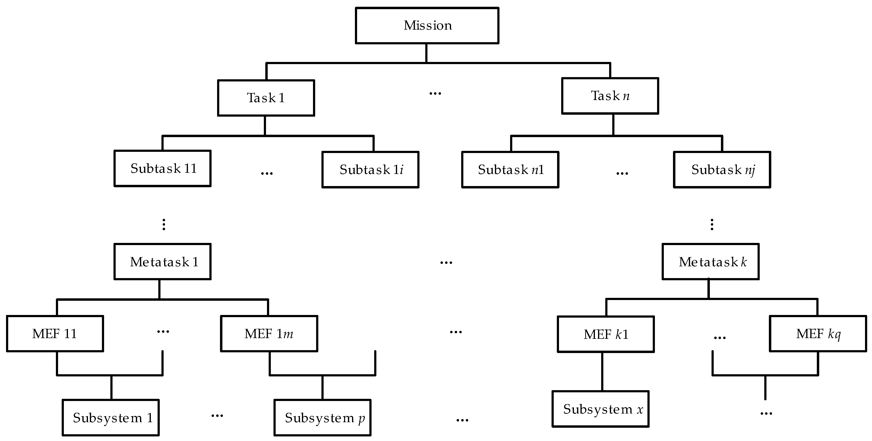
2. Hierarchical Decomposition of the SUT’s Mission

In operational testing, SUT is required to perform the designated test activities in accordance with the mission profile, which delineates the SUT’s tasks, activities, frequencies, periods, environmental conditions, and operational contexts at each stage. Additionally, the mission profile specifies the operational activities and environmental conditions pertinent to specific tasks, organized according to a timeline [18]. Therefore, the SUT in this context can be considered a Phased Mission System (PMS), which may have different functional structures in different mission phases, requiring different subsystems to perform different MEFs, where MEF refers to the minimum set of functions that must be performed to accomplish the specified operational tasks [19]. The SUT in operational testing is given one or more missions to describe the critical tasks that must be accomplished to meet the user’s needs. The aim of the mission is explicit, while the specific ways of accomplishing the mission need not be explicit. For example, a certain type of carrier-based aircraft is required to provide close air-fire support for a ship formation. If there are insufficient test data for the SUT and other data sources must be found, it is not possible to measure similarity for the entire system, because only certain subsystems or components may be similar between the SUT and the comparison system.

As an illustration, the reliability of the 57 mm gun on the Littoral Combat Ship (LCS) can be assessed by combining it with the 57 mm gun test data from the National Security Cutter (NSC). Despite the fact that it may have been modified to fit different platforms, there are still considerable areas of commonality. The mission of the SUT is decomposed hierarchically into MEFs, which are then mapped to the subsystems. By comparing the mission profile with the decomposition structure, the subsystems involved in operational testing can be clearly presented, thus allowing the similarity factors between different subsystems to be targeted. The tree structure of mission decomposition is illustrated in Figure 1.

As illustrated in Figure 1, the mission of SUT is structured in accordance with the mission$\to$task$\to$subtask$\to$metatask$\to$MEF hierarchy, with a corresponding relationship between the MEFs and the subsystems. Furthermore, subtasks may also exist at multiple levels, and metatask is the task that do not necessitate further decomposition at a specific level of granularity. In operational tests, due to the characteristics of the PMS, the object of data combination is the subsystem.

3. Similarity Factor Calculation

This section provides a detailed account of the methodology employed in calculating the similarity factor. It begins by outlining the process of establishing a PT representation of the subsystem. This is followed by a description of the approach used to calculate distance, taking into account the external circumstance. The subsequent step is to present the MIP solution for calculating distance and deriving the similarity factor.

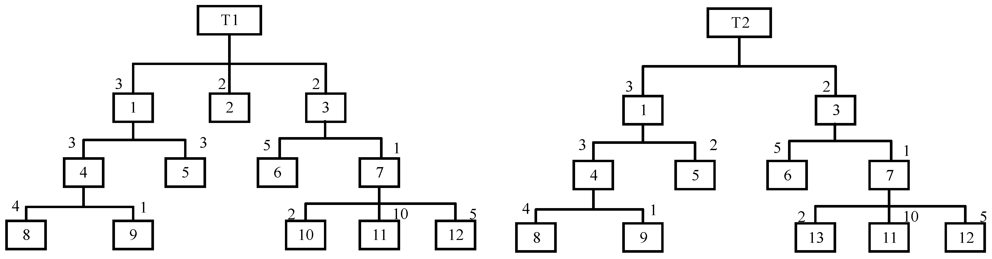
3.1. Establishment of PT Representation

The calculation of similarity factor requires the establishment of a suitable representation model to quantify the relevant elements. In addition to its application in the field of reliability assessment, similarity analysis has also been the subject of considerable interest among experts and scholars in the domains of design and manufacturing. Group technology [20] represents a traditional methodology for the analysis of product similarity. However, it necessitates a considerable investment of effort to ensure the continual refinement of the coding system. Similarity analysis based on functional features has also been developed in the field of design retrieval [21]. The challenge in applying it lies in the representation of codes for identifying functional features and the calculation of similarity based on functional feature ranking. Following years of practice and investigation, it has become evident that reliability is contingent upon the design, is refined during production, and is manifested in use [22]. The product structure can be conceptualized as a form of data that are shaped during the extended design and manufacturing process, reflecting the composition and interrelationships of the product’s internal components. Consequently, the product structure is inextricably linked to the reliability level, and research into its similarities has also garnered significant interest [23].

BOM was originally proposed by Dr. Orlicky [24] as a form of product data structure subordinate to the Material Requirements Planning (MRP) system commonly used for production planning and inventory control. BOM is a list of components, raw materials and their quantities required to produce the final product, which can be represented by an unordered root tree. The literature [25,26,27] employs BOM-based similarity metrics to ascertain the similarity between products. However, factors such as material composition, test circumstance, and operator level may influence product reliability data and thus warrant further investigation.

Figure 2 illustrates the BOM tree structure of two three-level subsystems, comprising eight and seven distinct basic components (numbered 8,9,5,2,6,10,11,12), respectively. The number adjacent to each component indicates the quantity required to form a parent component. For instance, component 1 is the parent of component 4 in T1, and three lots of component 4 are necessary to produce one component 1. Figure 2 is merely an illustrative example, and the actual scenario may encompass a greater number of components and hierarchies.

A BOM tree can be transformed into a PT, thereby facilitating the calculation of similarity factors. PT, also referred to as molecular evolutionary tree, is a method utilized in bioinformatics for the classification of a group of species that have descended from a common ancestor, as well as for the study of their evolutionary history [28]. Figure 3 depicts two PTs corresponding to Figure 2. The arbitrarily ordered numbers “①②③④⑤” indicate nodes, and the number of components associated with each node is shown in parentheses adjacent to the basic components.

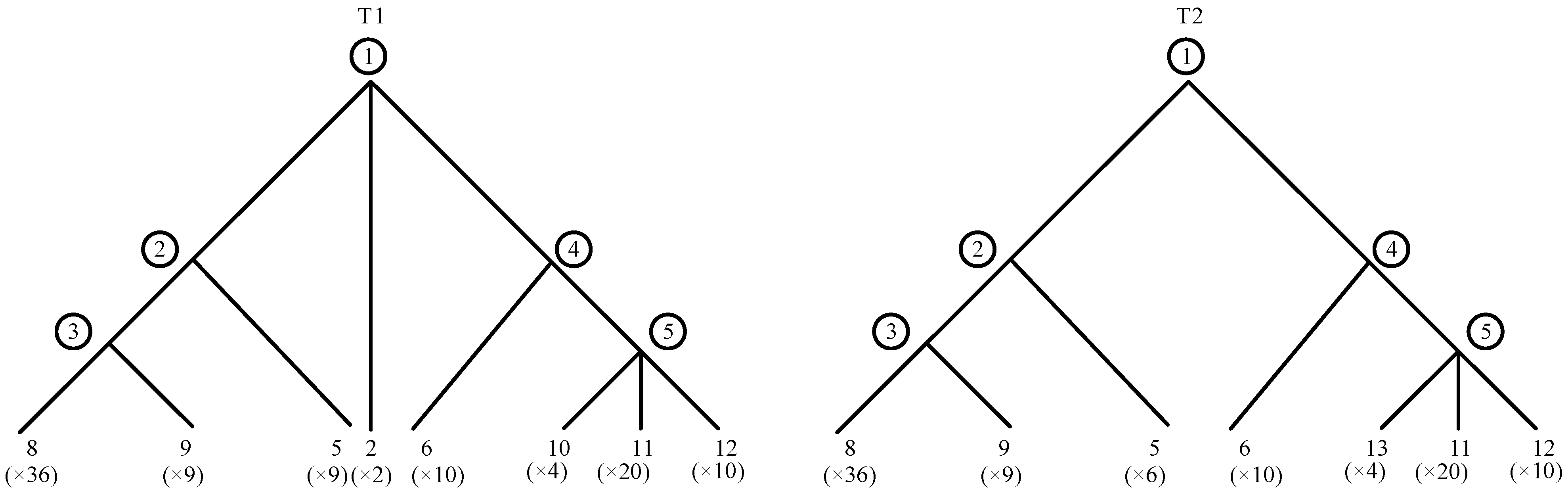
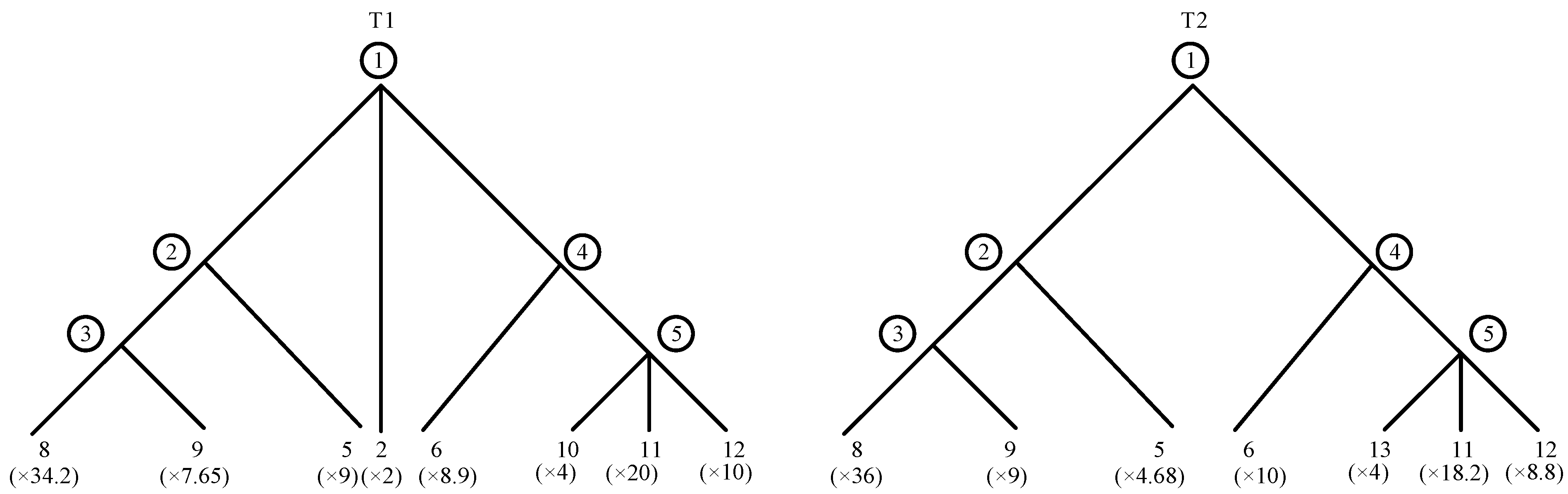
3.2. Distance Calculation Principle

Robinson–Foulds (RF) distance is a widely utilized metric for comparing PTs [29]. However, it is unable to account for quantitative differences between nodes and components. This limitation can be addressed by performing a bijective mapping between the subsystems [26]. Taking the PTs in Figure 3 as an example, each node in T1 is mapped to the most similar node in T2, and this process is repeated for each node in T2. The resulting mapping distances are then summarized in

Table 1. Summary of distances for mapping T1 nodes to T2 nodes.

Node in T1	Most Similar Node in T2	Component in T1 but Not in T2	Shared Component with Higher Quantity in T1	Level Difference	Quantity Difference	Distance
1	1	2, 10	5	1, 3, 2	2, 4, 3	4.83
2	2	-	5	1	3	3
3	3	-	-	-	-	0
4	4	10	-	2	4	2
5	5	10	-	1	4	4
Total						13.83

and

Table 2. Summary of distances for mapping T2 nodes to T1 nodes.

Node in T2	Most Similar Node in T1	Component in T2 but Not in T1	Shared Component with Higher Quantity in T2	Level Difference	Quantity Difference	Distance
1	1	13	-	3	4	1.33
2	2	-	-	-	-	0
3	3	-	-	-	-	0
4	4	13	-	2	4	2
5	5	13	-	1	4	4
Total						7.33

.

In Table 1, column 1 contains all the nodes in T1, and column 2 contains the nodes in T2 that are most similar to the nodes in column 1. This can be determined visually in simple PTs. Column 3 shows the components that are present in T1 but not in T2. Column 4 enumerates the components that are more abundant in T1 than in T2, among those that are shared by the corresponding nodes. Column 5 contains the hierarchical level differences between the components contained in columns 3–4 and the corresponding nodes. For example, if node ① is marked at level 0, then components 6, 10, and 11 are, in turn, marked at level 2, 3, and 3, respectively. Column 6 represents the number of components in column 3 and those in column 4 in T1 over T2, respectively. Column 7 denotes the mapping distance of the corresponding node, which is the summation resulting from dividing the corresponding elements in columns 6 and 5. The meanings of the columns in Table 2 are analogous to those expressed above.

As evidenced by Table 1 and Table 2, the distance between corresponding nodes is determined by the discrepancy in components and the structural characteristics of the node, irrespective of the designation of the intermediate node. This is a significant attribute of PT. For example, the node ⑤ in Figure 3 corresponds to component 7 in Figure 2. However, the components that comprise it in the two subsystems are distinct, which may introduce ambiguity in other similarity analysis methods. The question of whether the numbering of component 7 in the two subsystems should be consistent or not will yield disparate results. The method presented in this paper will remain unaffected by this discrepancy. In addition, the basic distance between different components is 1, which needs to be multiplied by the quantity difference and divided by the hierarchical level difference. For different components, an increase in quantity will correspondingly increase the distance between nodes, while the level difference is equivalent to the weight, and the smaller the difference, the greater the weight. In accordance with the data presented in Table 1 and Table 2, the distance between the subsystems can be calculated as the sum of all distances in both mapping directions, resulting in a total distance of 21.66.

In addition to being determined by intrinsic attributes such as structure, material, function, design principles, and working principles, the similarity factor may also be affected by external factors such as the working circumstance, the operator level, and interference from other subsystems within the SUT. These external factors can be considered as the external circumstance. In the PT, it can be posited that the basic components with the same number have essentially the same intrinsic attributes. Consequently, the same components operating in disparate external circumstance can be regarded as representing different working modes of the components. A study [23] presents a methodology for calculating the product similarity of components in disparate operational modes, which entails initially calculating the similarity factor of the components across various operational modes and subsequently multiplying the number of components in the compared products by the aforementioned similarity factor to derive the equivalent number of components. Nevertheless, when the number of components in the compared product is greater than that in the original product, it results in a situation where the similarity between the two products is greater than it would be if the working mode were not taken into account. This is evidently illogical. In this paper, it is assumed that a similar factor ${\rho }_i\left(0<{\rho }_i\le 1\right)$ has been obtained for the influence of the external circumstance on the reliability of two components numbered i in two PTs. The smaller quantity is multiplied by ${\rho }_i$ and regarded as the equivalent quantity. If the quantities are equal, either one is multiplied by ${\rho }_i$. Take Figure 3 as an example. Assuming that $\left({\rho }_8,{\rho }_9,{\rho }_5,{\rho }_6,{\rho }_{11},{\rho }_{12}\right)$ = (0.95, 0.85, 0.78, 0.89, 0.91, 0.88), the aforementioned method can be employed to modify Figure 3 into Figure 4. At this time, the distance is 36.065, which shows that the distance between subsystems will increase when considering the difference in the influence of the external circumstances.

The value of factor ${\rho }_i$ affects the final distance and should therefore be carefully considered in practical applications. The subjective experience of engineering experts is an important type of information, and it is common practice to assign a value to it after analysis and discussion.

3.3. MIP Solution of Distance and Determination of Similarity Factor

The preceding Section 3.2 presents the fundamental principle for calculating the distance between subsystems, taking into account the external circumstances. In operational testing, the SSUT is typically more complex, making it challenging to identify the most similar node through observation when performing node mapping, particularly when the external circumstance is taken into account. In such a case, the distance can be solved using MIP.

3.3.1. Matrix Encoding Corresponding to PT

MIP is an extension of linear programming, wherein decision variables encompass both continuous and discrete types [30]. Prior to solving the distance using MIP, the PT must be converted to matrix form. The conversion process is outlined below:

Step 1: Create matrices ${\mathit{M}}_1={\left[m_{ij}\right]}_{p\times q}$ and ${\mathit{M}}_2={\left[w_{bj}\right]}_{k\times q}$ corresponding to two PTs. The $i$-th ($b$-th) row of ${\mathit{M}}_1$(${\mathit{M}}_2$) corresponds to the node $i$($b$) of the PT. $p$($k$) is the total number of nodes, while $q$ denotes the total number of component numbers. All component numbers should be arranged in ascending order, and the values assigned to the matrix ${\mathit{M}}_1$ should be determined in accordance with the following Equation:

$$\left\{\begin{array}{l}{m}_{ij}=0\mathrm{node}i\mathrm{does}\mathrm{not}\mathrm{contain}\mathrm{the}j\mathrm{-th}\mathrm{component}\\ m_{ij}=1\mathrm{else}\end{array}\right.$$

(1)

Subsequently, the matrix ${\mathit{M}}_2$ should be assigned values in a similar manner.

Step 2: In the matrix ${\mathit{M}}_1$ resulting from step 1, the element $m_{ij}$ is to be replaced with $m_{ij}/l_{ij}$, where $l_{ij}$ is the hierarchical level difference between the j-th component and node i. The same replacement process is to be applied to the elements in matrix ${\mathit{M}}_2$.

Step 3: For matrix ${\mathit{M}}_1$ from step 2, multiply the elements in the j-th column by the equivalent quantity of the j-th component in the corresponding subsystem (taking into account the external circumstance). The same process is to be repeated for the elements in matrix ${\mathit{M}}_2$.

PTs depicted in Figure 4 can be converted into two matrices by following the aforementioned steps:

$${\mathit{M}}_1=\left[\begin{array}{ccccccccc}2& 4.5& 4.45& 11.4& 2.55& 4/3& 20/3& 10/3& 0\\ 0& 9& 0& 17.1& 3.825& 0& 0& 0& 0\\ 0& 0& 0& 34.2& 7.65& 0& 0& 0& 0\\ 0& 0& 8.9& 0& 0& 2& 10& 5& 0\\ 0& 0& 0& 0& 0& 4& 20& 10& 0\end{array}\right]$$

(2)

$${\mathit{M}}_2=\left[\begin{array}{ccccccccc}0& 2.34& 5& 12& 3& 0& 18.2/3& 8.8/3& 4/3\\ 0& 4.68& 0& 18& 4.5& 0& 0& 0& 0\\ 0& 0& 0& 36& 9& 0& 0& 0& 0\\ 0& 0& 10& 0& 0& 0& 9.1& 4.4& 2\\ 0& 0& 0& 0& 0& 0& 18.2& 8.8& 4\end{array}\right]$$

(3)

3.3.2. MIP Construction and Similarity Factor Calculation

Construct the following MIP optimization model based on matrices ${\mathit{M}}_1$ and ${\mathit{M}}_2$:

$$\begin{array}{l}\mathrm{Minimize}{\displaystyle \sum _{i=1}^p{\displaystyle \sum _{b=1}^k{x}_{ib}}}+{\displaystyle \sum _{b=1}^k{\displaystyle \sum _{i=1}^p{y}_{bi}}}\\ s.t.\left\{\begin{array}{l}{x}_{ib}+\mathrm{C}\left(1-z_{ib}\right)\ge {\displaystyle \sum _{j=1\left|m_{ij}\ge w_{bj}\right.}^q\left(m_{ij}-w_{bj}\right),\forall i=1,\dots ,p,\forall b=1,\dots ,k}\\ y_{bi}+\mathrm{C}\left(1-e_{bi}\right)\ge {\displaystyle \sum _{j=1\left|w_{bj}\ge m_{ij}\right.}^q\left(w_{bj}-m_{ij}\right),\forall b=1,\dots ,k,\forall i=1,\dots ,p}\\ {\displaystyle \sum _{b=1}^k{z}_{ib}=1,\forall i=1,\dots ,p}\\ {\displaystyle \sum _{i=1}^p{e}_{bi}=1,\forall b=1,\dots ,k}\end{array}\right.\end{array}$$

(4)

where the meanings of $p,k,q,m_{ij}$ and $w_{bj}$ are the same as in Section 3.3.1. If node i is mapped to node b, the value of $z_{ib}$ is 1; otherwise, it is 0. If node b is mapped to node i, the value of $e_{bi}$ is 1; otherwise, it is 0. $x_{ib}$ indicates the distance from node i to node b, and $y_{bi}$ indicates the distance from node b to node i. The objective function is the sum of the distances of all mappings, i.e., the distance between the two subsystems, in Equation (4). The first two inequalities within the constraint define $x_{ib}$ and $y_{bi}$, respectively, while the decision variables $z_{ib}$ and $e_{bi}$ in conjunction with constant C, which takes a large value, are used to ensure that $x_{ib}$ and $y_{bi}$ are assigned 0 when the distance between two nodes that are not mapped to each other is to be computed. The final two equations of the constraint serve to guarantee that each node is mapped to a single node.

In the MIP model, since each node of the two PTs is mutually mapped, the total number of decision variables becomes O(p × q), while the total number of constraints amounts to O(p + q). For complex structures where p and q take large values, solving the MIP model proves computationally challenging. To mitigate it, the COIN-OR Branch-and-Cut (CBC) solver is employed. CBC synergistically integrates the Branch-and-Bound method with Cutting Plane techniques to address complex MIP problems with precision [31]. Within the Branch-and-Bound framework, the branching count correlates with variable scale, yielding a theoretical complexity of O(p × q). Each branch requires solving a linear programming (LP) relaxation subproblem, typically with complexity O(m³) (m = O(p × q)). This nominally results in a theoretical total complexity of O(n⁶) for p ≈ q = n. However, the hierarchical nature of PTs and problem sparsity substantially reduce computational burdens: (1) Many variables and constraints become inherently irrelevant. For example, if a parent node is not mapped to a target tree node, its child nodes are automatically pruned. (2) Differences in low-level nodes contribute minimally to the global objective function, allowing heuristic pruning to further reduce branching counts. These optimizations degrade the practical complexity of LP subproblems, resulting in a total complexity far below O(n⁶).

Specifically, the optimization problem shown in Equation (4) can be expeditiously resolved during the programming implementation via the Python 3.11.7 language by importing the function ‘LpProblem’ from the module ‘pulp’ [32]. Upon feeding matrices ${\mathit{M}}_1$ and ${\mathit{M}}_2$ into the MIP model, the resulting distance between the two subsystems is 36.071. The similarity factor between them is:

$$s={\displaystyle \frac{D_{\max }-D}{D_{\max }}}$$

(5)

where $D_{max}$ represents the maximum possible distance between two subsystems, which is equal to the sum of all elements of matrices ${\mathit{M}}_1$ and ${\mathit{M}}_2$. This represents the situation when all nodes do not match at all. $D$ is the result of the distance between the subsystems. For matrices ${\mathit{M}}_1$ and ${\mathit{M}}_2$, D_max = 329.26 and s = 0.89.

4. Reliability Assessment Model

Assuming that there are I similar subsystems for a given SSUT, collect test data for these I + 1 subsystems and establish a data model $\left(t_a,{\delta }_a,s_a\right)$, where $a$ = 1, $\cdots$, and d, and d is the data size. $t_a$ is the observation time for a subsystem, ${\delta }_a$ is an indicator that takes 1 if $t_a$ is a failure data value and takes 0 if $t_a$ is a right-censored data value. $s_a$ is the similarity factor of the subsystem to which the data belong, and takes 1 when the data belong to the SSUT.

As the Weibull distribution is a prevalent tool in the field of reliability engineering and is intimately associated with other distribution types, including the exponential distribution and the Gamma distribution [33], this paper employs a two-parameter Weibull distribution to model the failure time, utilizing the following probability density function (p.d.f.):

$$f(t\left|h,\lambda \right.)={\displaystyle \frac{h}{\lambda }}{\left({\displaystyle \frac{t}{\lambda }}\right)}^{h-1}\exp \left(-{\left({\displaystyle \frac{t}{\lambda }}\right)}^h\right)$$

(6)

where h > 0, λ > 0 and t > 0 represent the shape parameter, scale parameter and failure time. The reliability function and the mathematical expectation of failure time are

$$R(t\left|h,\lambda \right.)=\exp \left(-{\left({\displaystyle \frac{t}{\lambda }}\right)}^h\right)$$

(7)

$$\mathrm{E}(T)=\lambda \mathsf{\Gamma }\left(1+{\displaystyle \frac{1}{h}}\right)$$

(8)

where $\mathsf{\Gamma }\left(\cdot \right)$ is the Gamma function. While there are some discrepancies in the failure-time distribution parameters between similar subsystems, their test data can be regarded as originating from the same population at a specific significance level, and there should also be some kind of correlation between the distribution parameters. In this paper, we employ the corresponding trick of Weibull survival regression to consider the similarity factor as a covariate. Within the reliability assessment framework, the similarity factor $s_a$ can be conceptualized as a design-equivalence acceleration factor, capturing structural and functional commonalities between subsystems. The relationship between the failure time $t_a$ and $s_a$ is modeled using a log-location-scale regression [34], a type of accelerated failure time (AFT) model. Specifically, the logarithmic failure time is expressed as:

$$\log (t_a)={\alpha }_1+{\beta }_1{s}_a+{\tau }_a{W}_a$$

(9)

where α₁ is the logarithm of the baseline failure time, β₁ is the effect coefficient of $s_a$, $W_a$ is the random error term following a standard extreme value (SEV) distribution, and ${\tau }_a$ is the scale parameter modulating the variability of $W_a$. By transforming Equation (9), the p.d.f. of $t_a$ can be derived as:

$$f\left(t_a\left|{\tau }_a,{\alpha }_1,{\beta }_1\right.\right)={\displaystyle \frac{1}{{\tau }_a{t}_a}}\exp \left({\displaystyle \frac{\log t_a-{\alpha }_1-{\beta }_1{s}_a}{{\tau }_a}}\right)\cdot \exp \left[-\exp \left({\displaystyle \frac{\log t_a-{\alpha }_1-{\beta }_1{s}_a}{{\tau }_a}}\right)\right]$$

(10)

This formulation corresponds to a Weibull distribution with scale parameter $\exp ({\alpha }_1+{\beta }_1{s}_a)$ and shape parameter $1/{\tau }_a$.

Traditional AFT models assume ${\tau }_a$ remains constant across acceleration factors, implying uniformity in failure mechanisms. However, structural disparities among similar subsystems may lead to divergent failure mechanisms. To address this, prior studies [35,36,37] suggest modeling the shape parameter as a function of $s_a$:

$$\log {\tau }_a=\log ({\displaystyle \frac{1}{h_a}})={\alpha }_2^{\prime }+{\beta }_2^{\prime }{s}_a$$

(11)

It allows $h_a$ to adapt to variations in $s_a$, thereby capturing shifts in failure mechanisms. Notably, when ${\beta }_2^{\prime }$ = 0, this model reduces to the constant shape-parameter assumption. The combined effects of $s_a$ on the Weibull parameters are then summarized as:

$$\left\{\begin{array}{c}{\lambda }_a=\exp \left({\alpha }_1+{\beta }_1{s}_a\right)\\ h_a=\exp \left({\alpha }_2+{\beta }_2{s}_a\right)\end{array}\right.$$

(12)

Subsequently, the likelihood of parameters α₁, β₁, α₂ and β₂ is derived as follows:

$$\begin{array}{ll}L({\alpha }_1,{\beta }_1,{\alpha }_2,{\beta }_2\left|D_a\right.)=& {{\displaystyle \prod _{a=1}^d\left[\begin{array}{l}\frac{\exp \left({\alpha }_2+{\beta }_2{s}_a\right)}{\exp \left({\alpha }_1+{\beta }_1{s}_a\right)}{\left[\frac{t_a}{\exp \left({\alpha }_1+{\beta }_1{s}_a\right)}\right]}^{\exp \left({\alpha }_2+{\beta }_2{s}_a\right)-1}\\ \cdot \exp \left(-{\left(\frac{t_a}{\exp \left({\alpha }_1+{\beta }_1{s}_a\right)}\right)}^{\exp \left({\alpha }_2+{\beta }_2{s}_a\right)}\right)\end{array}\right]}}^{{\delta }_a}\\ & \cdot {\left[\exp \left(-{\left({\displaystyle \frac{t_a}{\exp \left({\alpha }_1+{\beta }_1{s}_a\right)}}\right)}^{\exp \left({\alpha }_2+{\beta }_2{s}_a\right)}\right)\right]}^{1-{\delta }_a}\end{array}$$

(13)

where Da = $\left(t_a,{\delta }_a,s_a\right)$.

The selection of prior distributions should balance parameter physical interpretability with overfitting mitigation requirements. Parameters α₁ and α₂ represent the logarithmic values of the baseline failure time and baseline shape parameter, respectively. These must cover reasonable logarithmic ranges in engineering contexts while avoiding extreme values. The normal distribution, characterized by symmetry and smooth decay properties, provides flexibility to span plausible parameter ranges while constraining deviations from physical reality through variance regularization. Thus, α₁ and α₂ are assigned normal distributions, specified as α₁~N(μ₁, σ₁²) and α₂~N(μ₂, σ₂²). Parameters β₁ and β₂ reflect the regulatory effects of the similarity factor $s_a$ on the lifetime distribution. Given the “dominance of commonality over variability” among similar subsystems (e.g., modular design inheritance), these coefficients should exhibit small absolute values. The Laplace distribution, with its sharp peak and heavy-tailed properties, concentrates probability mass near the mean while exponentially attenuating tail probabilities [38]. This structure suppresses interference from anomalous similarity factors, thereby mitigating overfitting. Therefore, parameters β₁ and β₂ are assigned Laplace distributions, specified as β₁~Lap(a₁, b₁) and β₂~Lap(a₂, b₂).

In accordance with Bayesian theory, the joint posterior distribution of (α₁, β₁, α₂, β₂) is given by:

$$\begin{array}{c}\pi \left({\alpha }_1,{\beta }_1,{\alpha }_2,{\beta }_2\left|D_a\right.\right)\propto L({\alpha }_1,{\beta }_1,{\alpha }_2,{\beta }_2\left|D_a\right.)\cdot \varphi ({\displaystyle \frac{{\alpha }_1-{\mu }_1}{{\sigma }_1}})\cdot l({\beta }_1)\\ \cdot \varphi ({\displaystyle \frac{{\alpha }_2-{\mu }_2}{{\sigma }_2}})\cdot l({\beta }_2)\end{array}$$

(14)

where $\varphi$ is the standard normal distribution p.d.f. l(β₁) is the Laplace p.d.f. with expression as:

$$l({\beta }_1\left|a_1\right.,b_1)={\displaystyle \frac{1}{2b_1}}\exp \left(-\left|{\beta }_1-a_1\right|/b_1\right),-\infty <{\beta }_1<\infty$$

(15)

The expression for l(β₂) follows analogously.

The complex form of Equation (14) makes it difficult to give a closed expression, which can be sampled from the joint posterior distribution using MCMC. Specifically, the No-U-Turn Sampler (NUTS) is employed to execute the sampling process. NUTS is an extension of the HMC algorithm [39]. It consists of a sequence of steps based on first-order gradient information, effectively circumventing the random wandering behavior and parameter sensitivity commonly observed in alternative MCMC approaches. Specifically, its dual averaging algorithm enables the automatic calibration of the step size ϵ, thereby eliminating the sensitivity associated with manual configuration of it, while the U-turn criterion and tree-depth constraint dynamically regulate computational costs, allowing the trajectory length L to adapt to the complexity of the posterior distribution. Consequently, it can converge more rapidly to high-dimensional target distribution. Bayes point estimates for the parameters α₁, β₁, α₂, and β₂ can be readily obtained from the posterior samples. The sampling process of NUTS integrates Hamiltonian dynamics simulation and a dynamic path-termination strategy from HMC, whose core procedural steps are as follows:

Step 1: Parameter and momentum initialization. Starting from the initial parameter vector ${\mathsf{\theta }}^{(0)}=\left({\alpha }_1^{(0)},{\beta }_1^{(0)},{\alpha }_2^{(0)},{\beta }_2^{(0)}\right)$, randomly sample the momentum vector $\mathit{r}=\left(r_{{\alpha }_1},r_{{\beta }_1},r_{{\alpha }_2},r_{{\beta }_2}\right)\sim \mathrm{N}(0,\mathbf{I})$, where I denotes the identity matrix.

Step 2: Hamiltonian system construction. Construct the energy function as:

$$H\left(\mathsf{\theta },\mathit{r}\right)=-\log \pi (\mathsf{\theta }\left|D_a\right.)+{\displaystyle \frac{1}{2}}{\displaystyle \sum _{k\prime }{r}_{k\prime }^2}$$

where $-\log \pi (\theta \left|D_a\right.)=-\log \pi (D_a\left|\mathsf{\theta }\right.)-{\displaystyle {\sum }_{k\prime }\log \pi ({\theta }_{k\prime })}$ is the negative log-posterior, and k′ is the element index within the corresponding vector. The gradient of the log-posterior decomposes into partial derivatives with respect to individual parameters as:

$${\nabla }_{\mathsf{\theta }}\log \pi (\mathsf{\theta }\left|D_a\right.)=\left({\displaystyle \frac{\partial \log \pi }{\partial {\alpha }_1}},{\displaystyle \frac{\partial \log \pi }{\partial {\beta }_1}},{\displaystyle \frac{\partial \log \pi }{\partial {\alpha }_2}},{\displaystyle \frac{\partial \log \pi }{\partial {\beta }_2}}\right)$$

Step 3: Binary-tree recursive construction. Starting from the current state (θ, r), perform a leapfrog integration step (step size ϵ) and generate a new state through the following three-phase update:

Half-step momentum update: $r_{k\prime }\leftarrow r_{k\prime }+{\displaystyle \frac{\epsilon }{2}}\cdot {\displaystyle \frac{\partial \log \pi }{\partial {\theta }_{k\prime }}}$

Full-step parameter update: ${\theta }_{k\prime }\leftarrow {\theta }_{k\prime }+\epsilon \cdot r_{k\prime }$

Remaining half-step momentum update: $r_{k\prime }\leftarrow r_{k\prime }+{\displaystyle \frac{\epsilon }{2}}\cdot {\displaystyle \frac{\partial \log \pi }{\partial {\theta }_{k\prime }}}$

Randomly select the expansion direction (forward/backward) for each parameter during each recursive path expansion. Synchronously check the U-turn condition across all parameters: ${\displaystyle {\sum }_{k\prime }\left({\theta }_{k\prime }^{+}-{\theta }_{k\prime }^{-}\right)\cdot r_{k\prime }^{-}}<0$ or ${\displaystyle {\sum }_{k\prime }\left({\theta }_{k\prime }^{+}-{\theta }_{k\prime }^{-}\right)\cdot r_{k\prime }^{+}<0}$, where ${\theta }_{k\prime }^{+}$ and ${\theta }_{k\prime }^{-}$ denote the endpoint states of the current trajectory. If the U-turn condition is met, terminate path expansion and discard the newly generated states. The effective number of steps L is then $2^{j\prime }-1$, where j′ represents the height of the binary tree.

Step 4: Candidate state selection. Define a random variable $u\sim$$\mathrm{Uniform}\left[0,\exp \left(-H(\mathsf{\theta },\mathit{r})\right)\right]$ and sample from it. Filter states satisfying $H(\theta \prime ,r\prime )\le -\log u$, then randomly draw the new parameter ${\mathsf{\theta }}_{\mathrm{new}}$ from the valid candidate set.

Step 5: Adaptive step-size tuning. The step size ϵ is dynamically adjusted via the dual averaging algorithm to steer the average acceptance rate toward a preset target. The dual averaging update rule is:

$$\log {\epsilon }_{t+1}=\mu -{\displaystyle \frac{\sqrt{t}}{\gamma }}{\overline{H}}_t,\mu =\log (10{\epsilon }_0)$$

It is of greater significance that Bayes point estimates and credible intervals (including equal-tailed intervals (ETIs) and highest posterior density (HPD) intervals [40]) for reliability and failure time can be obtained from the posterior sample. The specific steps are as follows:

Step 1: Let v = 1.

Step 2: Draw the parameter sample $\{{\alpha }_1^{\left(v\right)},{\beta }_1^{\left(v\right)},{\alpha }_2^{\left(v\right)}$,${\beta }_2^{\left(v\right)}$} from the posterior distribution shown in Equation (14) using NUTS.

Step 3: Convert parameter sample into reliability metrics R^(v) and E^(v)(T) via Equations (7), (8) and (12). Increment v by 1.

Step 4: Repeat steps 2–3 until v = N, yielding complete sample sets ${\left\{R^{\left(v\right)}\right\}}_{v=1}^N$ and ${\left\{E^{\left(v\right)}\right\}}_{v=1}^N$.

Step 5: Compute posterior-mean estimates as:

$$\widehat{R}={\displaystyle \frac{1}{N}}{\displaystyle \sum _{v=1}^N{R}^{(v)}},\hat{\mathrm{E}}\left(T\right)={\displaystyle \frac{1}{N}}{\displaystyle \sum _{v=1}^N{\mathrm{E}}^{(v)}(T)}$$

(16)

Step 6: Sort $\left\{R^{\left(v\right)}\right\}$ and $\left\{{\mathrm{E}}^{\left(v\right)}\right\}$ in ascending order as R₍₁₎ ≤ R₍₂₎ ≤ $\cdots$R_(N) and E₍₁₎(T) ≤ E₍₂₎ (T) ≤ $\cdots$E_(N) (T). Then, the (1 − α) × 100% ETI are:

$$\left[R_{(⌊\alpha N/2⌋)},R_{(⌈N-\alpha N/2⌉)}\right],\left[{\mathrm{E}}_{(⌊\alpha N/2⌋)},{\mathrm{E}}_{(⌈N-\alpha N/2⌉)}\right]$$

(17)

where $⌊·⌋$ and $⌈·⌉$ denote floor and ceiling functions, respectively.

Step 7: Determine the coverage sample count of HPD interval $z=⌈N\cdot (1-\alpha )⌉$. For sorted {R_(v)}, compute lengths of all contiguous intervals [R_(v), R_(v+z−1)] as L_v = R_(v+z−1) − R_(v); then, the interval with minimal L_v is the HPD interval. Repeat for $\left\{{\mathrm{E}}^{\left(v\right)}\right\}$.

Posterior predictive checks are essential for assessing the validity of the model. The Bayesian p-value serves as a useful metric to evaluate the goodness-of-fit between the model and the data. Following the steps outlined above (Step 1–4), posterior samples of the Weibull parameters, denoted as ${\left\{m^{\left(v\right)}\right\}}_{v=1}^N$ and ${\left\{{\lambda }^{\left(v\right)}\right\}}_{v=1}^N$, are obtained. For each parameter sample ($m^{\left(v\right)}$, ${\lambda }^{\left(v\right)}$), a set of posterior predictive data $t_{\mathrm{rep}}^{\left(v\right)}\sim \mathrm{Weibull}(m^{\left(v\right)},{\lambda }^{\left(v\right)})$ is generated, where the sample size of it typically matches that of the observed data. Then, the same statistic (e.g., mean, median, or standard deviation) for both the observed data and posterior predictive data, denoted as $S_{\mathrm{obs}}^{\left(v\right)}$ and $S_{\mathrm{rep}}^{\left(v\right)}$, is computed. The Bayesian p-value is calculated as the proportion of posterior predictive statistics exceeding the observed statistic:

$$p_{\mathrm{B}}={\displaystyle \frac{1}{N}}{\displaystyle \sum _{v=1}^N\mathrm{I}\left(S_{\mathrm{rep}}^{(v)}\ge S_{\mathrm{obs}}^{(v)}\right)}$$

where $\mathrm{I}\left(\cdot \right)$ is the indicator function (equal to 1 if the condition holds, otherwise 0). As shown in the equation, a $p_{\mathrm{B}}$-value of 0.5 indicates a perfect fit.

5. Numerical Experiments

5.1. Application of the Proposed Method

This subsection provides an application of the proposed method, utilizing the operational test of a particular type of equipment as a case study. The mission of this equipment is assumed to be breaching opponent’s defensive position, which is decomposed hierarchically in accordance with the method described in Section 2, and the simplified tree structure is illustrated in Figure 5.

The lower-level decompositions of the “Buildup” and “Assault” tasks are simplified in Figure 5 because this subsection employs the “Hydraulic subsystem” under the “Firepower preparation” task branch as an illustrative example. It comprises a hydraulic pump, a control component, and a hydraulic connector and pipe. Additionally, five distinct variants of the equipment are available, each exhibiting variations in the hydraulic subsystem. The hydraulic subsystems are designated as H1–H6, with H1 representing the SSUT. Their BOM tree structures are illustrated in Figure 6. Some components in the BOMs are simplified. Some identical or inconveniently disclosed components are removed, and the different components are highlighted to maintain the complexity of the method verification process. However, it does not indicate that the proposed method is incapable of handling more complex hierarchies. The six hydraulic subsystems contain a total of 21 different components, each of which is assigned a distinct number, as illustrated in

Table 3. Basic components’ names and their assigned numbers.

Name	Assigned Number	Name	Assigned Number
Pressure control valve	1	Copper pipe	12
Ceramic cartridge	2	Steel chrome-plated connector	13
Valve body	3	Housing partition manifold	14
Spring	4	Turret partition manifold	15
Direction control valve	5	Steel pipe	16
Cylinder block	6	Cooler	17
Guide sleeve	7	Copper pipe	18
Mandrel	8	Reinforced armor	19
Port plate	9	Copper alloy cartridge	20
Suction valve	10	Brass connector	21
Discharge valve	11

. The PT corresponding to each hydraulic system is depicted in Figure 7.

Let H1 be paired with H2~H6, respectively, and calculate the similarity factors according to the method described in Section 3. The distances between H1 and H2~H6 can be calculated as 15.67, 21.33, 12.83, 15.50, and 42.50, respectively. The maximum possible distances are 212.33, 225.33, 228.83, 220.50, 217.50. Substituting the value of D_max as 228.83 into Equation (5) yields the similarity factors, which are 0.93, 0.91, 0.95, 0.94 and 0.81, respectively. The result can also be visually perceived from Figure 7. Compared with H1, H6 is observed to lack components “2” and “13” and to have additional “20” and “21”. This discrepancy is more pronounced than that observed in the other subsystems, providing further evidence that this methodology is sound.

Following a period of deliberation, the engineering experts arrived at a consensus regarding the external circumstance impact on the same components, which is expressed in matrix form as follows:

$$\left[\begin{array}{ccccccccccccccc}0.86& 0.92& 0.95& 0.78& 0.95& 0.88& 0.82& 0.98& 0.74& 0.88& 0.77& 0& 0.75& 0.89& 0.91\\ 0.78& 0.75& 0.83& 0.76& 0.99& 0.89& 0.98& 0.94& 0.72& 0.97& 0.78& 0& 0.77& 0.93& 0.88\\ 0.87& 0.85& 0.88& 0.84& 0.83& 0.86& 0.92& 0.88& 0.75& 0.94& 0.94& 0.71& 0.78& 0.77& 0.98\\ 0.88& 0& 0.98& 0.91& 0.72& 0.92& 0.94& 0.93& 0.88& 0.79& 0.96& 0.73& 0.98& 0.83& 0.99\\ 0.99& 0& 0.89& 0.91& 0.88& 0.96& 0.82& 0.88& 0.76& 0.93& 0.81& 0.71& 0& 0.80& 0.75\end{array}\right]$$

(18)

The element in the i-th row and the j-th column of the matrix represents the similarity factor between two components numbered j in the hydraulic subsystems H(i + 1) and H1 with respect to the influence of the external circumstances. In considering the impact of the external circumstances on reliability, the distances between H1 and H2~H6 can be solved as 29.67, 29.05, 44.11, 45.94, and 59.57. The similarity factors are 0.87, 0.84, 0.81, 0.80, and 0.76, respectively.

Figure 8 illustrates the data pertaining to the six hydraulic subsystems. “×” represents the failure-time data, “•” represents the right-censored data, and subsystem number 1 corresponds to SSUT. Based on engineering experience, it can be inferred that the data follow a Weibull distribution.

NUTS is employed for sampling from the joint posterior distribution as shown in Equation (14). Given the absence of supplementary prior knowledge, the determination of hyperparameters should balance the dispersion characteristics of weakly informative priors with the conservatism requirements of engineering practice. Based on the test data characteristics (the maximum 462.02 h corresponding to logt_max = 6.14, and the minimum 7.4 h corresponding to logt_min = 2.0), the logarithmic baseline failure time α₁ is specified as α₁∼N(4, 8²). For the logarithmic baseline shape parameter α₂, operational testing typically involves small-batch prototype equipment, which predominantly operates in the infant mortality phase (h < 1) or random failure phase (h = 1). Even for similar subsystems in the wear-out phase, the shape parameter generally remains small. Thus, α₂∼N(0, 8²) is adopted. The effect coefficients for similarity factors (β₁, β₂) are both assigned Lap(0, 8). This configuration constrains the magnitude of similarity factor effects while preventing excessive model reliance on similarity factor differences through effective regularization. Figure 9 displays the posterior distribution curves of model parameters, annotated with posterior means and their 95% HPD intervals (denoted as HDI). Figure 10 presents the convergence diagnostics for the four parameters, generated using PyMC 5.18.2, a Python probabilistic programming library [41]. Figure 11 illustrates the time-dependent reliability function of the SSUT, comparing ETI with HPD intervals. The estimate of the expected failure time is 167.8 h, with a 95% ETI [126.90 h, 222.58 h] and HPD interval [123.44 h, 215.99 h]. Notably, the single failure observation for SSUT in Figure 8 renders maximum likelihood estimation statistically invalid under Weibull distribution assumptions due to insufficient data.

In the table shown in Figure 10, the explanations for some column headers are as follows:

SD: Standard deviation

MCSE Mean: Monte Carlo standard error of mean estimate

MCSE SD: Monte Carlo standard error of standard deviation estimate

ESS Bulk: Effective sample size for distribution bulk

ESS Tail: Effective sample size for distribution tails

R-hat: Gelman–Rubin statistic

The following three key findings serve as evidence of robust sampling performance and reliable parameter estimation:

(1) The ESS Bulk ranges from 1557 to 1628 (>1500), and the ESS Tail spans 1350 to 1908 (>1350). These metrics indicate sufficient sampling and high sampling efficiency.

(2) The maximum MCSE Mean/SD is 2.5% (β₂: 0.076/3.026), and the maximum MCSE SD/SD is 1.8% (β₂: 0.056/3.026), both below the 5%. This demonstrates highly reliable mean estimates and dispersion estimates of the parameters.

(3) All parameters have R-hat values very close to 1, indicating excellent convergence of the sampling chains.

5.2. Comparison of Methods

The calculation method of similarity factor is compared with the Jaccard similarity measure. The Jaccard coefficient J_xy between products x and y is calculated using the following equation:

$$J_{xy}={\displaystyle \frac{N_s}{N_s+N_b+N_c}}$$

(19)

where N_s is the number of components shared between products x and y. N_b is the number of components belonging to x but not y, and N_c is the number of components belonging to y but not x. J_xy is expressed only as the ratio between the number of shared components and the total number of components, regardless of the relationship between components. The Jaccard coefficients between H1 and H2–H6 are calculated using Equation (19), yielding values of 0.85, 0.81, 0.89, 0.87, and 0.65, respectively, in the absence of external circumstances. The results of the two methods indicate a consistent ability to distinguish similarities between H1 and H2–H6. However, a notable discrepancy is observed in the Jaccard coefficient between H6 and H1, which is too small and may result in the exclusion of H6 data during data collection. As illustrated in Figure 7, H6 and H1 exhibit a consistent hierarchy. Discrepancies exist in the constituent components 2, 15, 20, and 21. The weights of them differ depending on the hierarchical level. The Jaccard coefficient does not distinguish between them well, and exaggerates the weights of 2 and 20.

Simulation is used to verify the accuracy of the reliability assessment method in Section 4. Suppose that for SSUT, there are two similar subsystems. The similarity factors between subsystems 1–2 and SSUT are set to 0.78 and 0.95, respectively. The parameters in Equation (12) are set as α₁ = 5.26, β₁ = −0.65, α₂ = 0.38, and β₂ = 0.28, and the failure-time distribution parameters of the three subsystems are then solved. Subsequently, the failure-time data for the subsystems are generated, with SSUT collecting one data point and subsystems 1–2 collecting six and eight data points, respectively. Finally, the failure-time distribution parameters of SSUT are estimated according to the method described in Section 4, with the prior distributions of α₁, β₁, α₂, and β₂ specified as N(3.5, 10²), Lap(0, 8²), N(0, 8²), and Lap(0, 8²).

For comparison, the method described in the literature [16] is also employed for the estimation of the distribution parameters. Let θ = (h, λ), and the prior obtained from the data of the similar subsystem i′ is ${\pi }_{i^{\prime }}\left(\mathit{\theta }\right)$, i′ = 1, 2. Subsequently, the priors are combined equally into a single prior distribution $\pi \left(\mathit{\theta }\right)=0.5{\sum }_{i^{\prime }=1}^2\left[{s^{\prime }}_{i^{\prime }}{\pi }_{i^{\prime }}\left(\mathit{\theta }\right)+1-{s^{\prime }}_{i^{\prime }}\right]$, where ${s^{\prime }}_{i^{\prime }}$ is the “inheritance factor” and is equivalent to the similarity factor. The part inside the symbol “[]” of the equation is a mixture prior distribution, which contains an informative prior ${\pi }_{i^{\prime }}\left(\mathit{\theta }\right)$ and an uninformative prior represented by a uniform distribution. In accordance with Bayesian theory, the posterior distribution $\pi \left(\mathit{\theta }\left|D\right.\right)$ can be derived from the test data D of SSUT and $\pi \left(\mathit{\theta }\right)$, which can be used to estimate $\mathit{\theta }$.

Both the proposed method and the existing method need to employ NUTS for the purpose of sampling from $\pi \left(\mathit{\theta }\left|D\right.\right)$. Given that the status of SSUT and subsystems 1–2 can be interchanged, the parameters of subsystem 1–2 can also be estimated using the same method. To eliminate the influence of random effects, each method is repeated 100 times, and relative deviation between the estimated value and the true value is then subjected to statistical analysis. The results are presented in

Table 4. The results from the simulation study.

Subsystem	Parameter	Relative Deviation
		Existing Method	Proposed Method
SSUT	h	0.158	0.053
	λ	0.218	0.068
Subsystem 1	h	0.413	0.214
	λ	0.216	0.169
Subsystem 2	h	0.324	0.231
	λ	0.317	0.112

. It is evident that the absolute value of relative deviation of the proposed method is less than that of the existing method, indicating that it has a greater accuracy. The primary reason for this discrepancy is that, although the existing method integrates engineering data and expert insights into the determination of inheritance factor, it lacks the utilization of test data to align the relationship between inheritance factor and failure-time distribution parameters. In contrast, the proposed method can address this shortcoming, thereby conferring upon the reliability assessment model a degree of learning capacity.

5.3. Application Extensions

This section evaluates two scalability challenges: (1) computational efficiency under increasing subsystem hierarchy and node complexity, and (2) implementation strategies for handling missing and noisy test data.

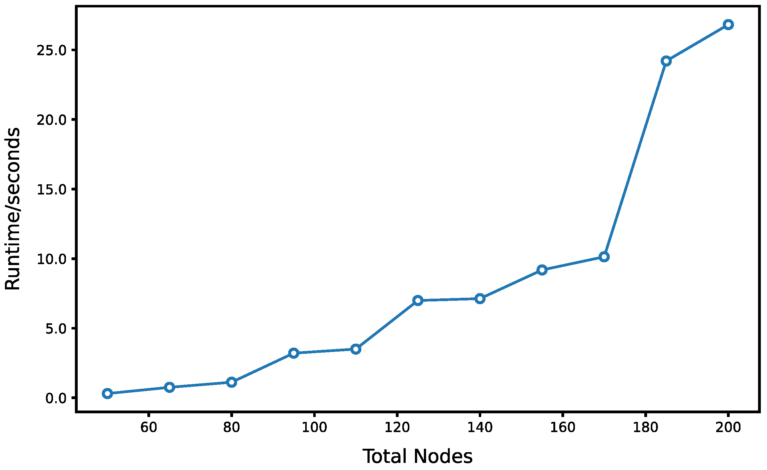
5.3.1. Computational Scalability in Complex Subsystems

This section achieves the correlation analysis between subsystem complexity and computational efficiency through the following steps:

First, set the number of nodes (including bottom-level component nodes) and maximum hierarchy depth, then construct a baseline PT through stochastic generation. Subsequently, while keeping the tree structure unchanged, implement controlled random modifications to the quantity of bottom-level components through random perturbations, obtaining a pair of PTs with identical structures but varying terminal quantities. This simplification focuses the study on the impact of structural complexity on computational efficiency. Next, apply the methodology described in Section 3 to perform matrix generation, MIP model solving, and record algorithm runtime. Testing is conducted on hardware configured with an Intel(R) Core (TM) i7-8565U CPU @ 1.80 GHz and 4.00 GB installed RAM (3.88 GB available). The total number of nodes is systematically varied, with each configuration undergoing 10 independent trials. Runtime measurements were then averaged across all repetitions for statistical reliability. The resultant computational efficiency trends are demonstrated in Figure 12.

As shown in Figure 12, the MIP model solution time demonstrates a distinct segmented growth pattern as the total node count varies with the range of [50, 200]. The solving duration exhibits a gradual upward trend in the 50–175 node interval, while experiencing a marked acceleration in growth rate between 175 and 200 nodes. The solution time peaks at 42.32 s when reaching the node count of 200. This phenomenon indicates that the MIP model possesses scalable adaptive capabilities for complex subsystems, implementing granularity control to optimize hierarchical structure design can effectively reduce node scale and improve computational efficiency.

5.3.2. Processing of Missing and Noisy Data

In real-world scenarios, missing data and noisy observations are common challenges that significantly impact reliability assessments. This section proposes targeted solutions by integrating the Bayesian modeling framework described in Section 4, and their effectiveness is validated through numerical experiments.

This study generates a reliability test dataset containing missing values, right censored data, and noise through parametric simulation. The generation process comprises the following steps: (1) Set regression coefficients as α₁ = 6.12, β₁ = −0.55, α₂ = 0.25, and β₂ = 0.35. (2) Create 12 subsystems (including 1 SSUT), with similarity factors for 11 subsystems sampled uniformly from [0.65, 1.0], while the SSUT is fixed at 1.0. (3) Simulate failure times for each subsystem using the Weibull distribution, introducing 15% right censoring. (4) Randomly remove 15% of the failure-time observations to simulate missing data, and superimpose Gaussian noise with a standard deviation of 10% on the remaining failure times. Through these procedures, a simulated dataset containing 120 entries was obtained, including 14 missing entries and 22 right-censored entries.

Considering the limited data volume of each subsystem, it is necessary to integrate the data from all subsystem into a single model. Building upon the reliability assessment model described in Section 4, this case treats the observed failure time $t_{\mathrm{obs},a}$ as a Gaussian noise model centered around the true failure time $t_{\mathrm{true},a}$, expressed as $t_{\mathrm{obs},a}\sim \mathrm{N}(t_{\mathrm{true},a},{\sigma }_{\mathrm{noise}}^2)$, where $t_{true,a}$ is treated as a latent variable. The joint prior distribution for all latent variables is defined as ${\displaystyle {\prod }_{a=1}^d\mathrm{Weibull}}(t_{\mathrm{ture},a}\left|h_a,{\lambda }_a\right.)$. According to Bayesian theory, the joint posterior distribution can be obtained as:

$$\begin{array}{l}\pi \left({\alpha }_1,{\beta }_1,{\alpha }_2,{\beta }_2,{\sigma }_{\mathrm{noise}},t_{\mathrm{ture}}\left|D\right.\right)\propto \pi ({\alpha }_1)\pi ({\beta }_1)\pi ({\alpha }_2)\pi ({\beta }_2)\pi ({\sigma }_{\mathrm{noise}})\\ \cdot {\displaystyle {\prod }_{a=1}^d\mathrm{Weibull}}(t_{\mathrm{ture},a}\left|h_a,{\lambda }_a\right.){\displaystyle \prod _{a\in \mathrm{obs}}\mathrm{N}(t_{\mathrm{obs},a}\left|t_{\mathrm{ture},a},\right.{\sigma }_{\mathrm{noise}}^2)}{\displaystyle \prod _{a\in \mathrm{cens}}\exp \left(-{\left(\frac{t_{\mathrm{cens},a}}{{\lambda }_a}\right)}^{h_a}\right)}\\ \cdot {\displaystyle \prod _{a\in \mathrm{missing}}\exp \left(-{\left(\frac{t_{\mathrm{true},a}}{{\lambda }_a}\right)}^{h_a}\right)}\end{array}$$

(20)

The prior distribution for parameters α₁, α₂, β₁, and β₂ are determined following the method outlined in Section 4. Since the variability of the noise is generally small compared the true failure times, a weakly informative prior N(0, 8²) can be assigned to ${\sigma }_{\mathrm{noise}}$.

The NUTS algorithm is employed for the posterior distribution sampling of parameters. In the presence of noise and missing values, it demonstrates high computational complexity and heightened sensitivity to parameter configurations, necessitating meticulous hyperparameter tuning. Regarding prior distribution selection, we adhere to the construction strategy outlined in Section 4, effectively integrating domain-specific engineering knowledge while maintaining weakly informative prior characteristics. Our experiments reveal that the dispersion level of weakly informative priors has limited impact on parameter estimation accuracy but significantly affects algorithmic convergence efficiency—priors with higher dispersion substantially increase required iteration counts. After careful consideration, the final-parameter prior distributions are established as α₁~N(4.6, 8²), β₁~Lap (0, 8), α₂~N(0, 8²), β₂~Lap (0, 8), and ${\sigma }_{\mathrm{noise}}$~N(0, 5²).

For the sampling configuration, four independent Markov chains were implemented with 2000 sampling iterations per chain (plus 1000 tuning iterations), with a target acceptance probability of 0.97. This empirically optimized configuration demonstrates that minor adjustments within this parameter neighborhood yield negligible impacts on posterior estimation. Convergence diagnostics, as shown in Figure 13, confirm full convergence: all parameters achieve R-hat statistics of 1.001 and effective sample sizes (ESS) exceeding 2000. Notably, parameter α₁ exhibits superior estimation precision compared to others, attributable to its structural centrality and strong identifiability in the model framework. Estimation biases in remaining parameters primarily stem from interactions between data missingness and noise.

To assess model goodness-of-fit, posterior predictive checks generate failure-time predictions incorporating observational noise. As shown in Figure 14, a comparative analysis of the observed data cumulative distribution curve against 100 posterior predictive curves demonstrates effective replication of key distributional characteristics. Bayesian posterior predictive checks yielded the following p-values: mean p-value = 0.679, median p-value = 0.597, and standard deviation p-value = 0.640. These results indicate (1) excellent capture of central tendency (median p ≈ 0.5); (2) minor systematic biases in distributional balance (right-skewed mean p > 0.6) and dispersion modeling (standard deviation p > 0.6). Potential sources of discrepancies include missing values, noise effects, and data multimodality (from multiple distinct Weibull distribution).

6. Conclusions

In operational testing scenarios, data from similar systems can effectively complement the test data of the SUT. This study proposes a novel reliability assessment framework that combines data from SSUT through systematic data combination. The mission of SUT is initially decomposed to identify SSUT that requires data combination operation. Subsequently, BOM trees of similar subsystems are matched to PTs. MIP is then employed to determine the distance between subsystems, thereby obtaining the similarity factors. The impact of the external circumstance on subsystem components is taken into account during the solution process. Ultimately, a reliability assessment model is constructed, and Bayesian theory and NUTS are utilized to obtain the reliability assessment results. Numerical experiments demonstrate the framework’s practical applicability and superior performance compared to conventional methods. Three conclusions were drawn as follows:

(1) Operational test constraints significantly challenge standalone reliability assessment. Data combination from similar systems emerges as an effective mitigation strategy, particularly beneficial for systems with limited test data availability.

(2) System reliability demonstrates strong dependence on structural configuration and operational environment. Matching the BOM tree of a subsystem to a PT enables MIP to rapidly and accurately solve the similar factors.

(3) It is essential to ascertain the relationship between the similarity factor and failure-time distribution parameters via the underlying system mechanisms, and should also be considered for learning from test data.

This work constitutes a critical component of our ongoing research program for operational reliability evaluation. Future efforts will focus on hierarchical reliability aggregation from subsystem to system level, ultimately determining mission reliability through comprehensive verification.

References

1. Dement, A.; Hartman, R. Operational suitability evaluation of a tactical fighter system. In Proceedings of the 3rd Flight Testing Conference and Technical Display, Las Vegas, NV, USA, 2–4 April 1986; p. 9753. [Google Scholar]
2. Li, J.; Nie, C.; Wang, L. Overview of weapon operational suitability test. In Proceedings of the 2016 International Conference on Artificial Intelligence and Engineering Applications, Hong Kong, China, 16–18 March 2016; Atlantis Press: Dordrecht, The Netherlands, 2016; pp. 423–428. [Google Scholar]
3. National Research Council; Division of Behavioral; Committee on National Statistics; Panel on Operational Test Design and Evaluation of the Interim Armored Vehicle. Improved Operational Testing and Evaluation and Methods of Combining Test Information for the Stryker Family of Vehicles and Related Army Systems: Phase II Report; National Academies Press: Washington, DC, USA, 2003. [Google Scholar]
4. Lee, B.; Seo, Y. A design of operational test & evaluation system for weapon systems thru process-based modeling. J. Korea Soc. Simul. 2014, 23, 211–218. [Google Scholar]
5. Ke, X.C. Reliability predictions of a canister cover based on similar product method. Environ. Adapt. Reliab. 2022, 40, 35–37. [Google Scholar]
6. Li, L.; Liu, Z.; Du, X. Improvement of analytic hierarchy process based on grey correlation model and its engineering application. ASCE-ASME J. Risk Uncertain. Eng. Syst. Part A Civ. Eng. 2021, 7, 04021007. [Google Scholar] [CrossRef]
7. Ahlgren, P.; Jarneving, B.; Rousseau, R. Requirements for a cocitation similarity measure, with special reference to Pearson’s correlation coefficient. J. Am. Soc. Inf. Sci. Technol. 2003, 54, 550–560. [Google Scholar] [CrossRef]
8. Xiang, S.; Nie, F.; Zhang, C. Learning a Mahalanobis distance metric for data clustering and classification. Pattern Recognit. 2008, 41, 3600–3612. [Google Scholar] [CrossRef]
9. Elmore, K.L.; Richman, M.B. Euclidean distance as a similarity metric for principal component analysis. Mon. Weather Rev. 2001, 129, 540–549. [Google Scholar] [CrossRef]
10. Li, J.; Dai, W. Multi-objective evolutionary algorithm based on included angle cosine and its application. In Proceedings of the 2008 International Conference on Information and Automation, Changsha, China, 20–23 June 2008; IEEE: Piscataway, NJ, USA, 2008; pp. 1045–1049. [Google Scholar]
11. Rui, H.D. Research on Reliability Growth AMSAA Model of Complex Equipment Based on Grey Information. Master’s Thesis, Nanjing University of Aeronautics and Astronautics, Nanjing, China, 2016. [Google Scholar]
12. Meeker, W.Q.; Escoba, L.A. Reliability: The other dimension of quality. Qual. Technol. Quant. Manag. 2004, 1, 1–25. [Google Scholar] [CrossRef]
13. Jin, S.; Chen, J.; Gu, R. Study on similarity criterion of equivalent life model of wind turbine main shaft bearing. Manuf. Technol. Mach. 2021, 7, 146–152. [Google Scholar]
14. Liu, Y.; Huang, H.Z.; Ling, D. Reliability prediction for evolutionary product in the conceptual design phase using neural network-based fuzzy synthetic assessment. Int. J. Syst. Sci. 2013, 44, 545–555. [Google Scholar] [CrossRef]
15. Fang, S.; Li, L.; Hu, B.; Chen, X. Evidential link prediction by exploiting the applicability of similarity indexes to nodes. Expert Syst. Appl. 2022, 210, 118397. [Google Scholar] [CrossRef]
16. Yang, J.; Shen, L.J.; Huang, J.; Zhao, Y. Bayes comprehensive assessment of reliability for eectronic products by using test information of similar products. Acta Aeronaut. Astronaut. Sin. 2008, 29, 1550–1553. [Google Scholar]
17. Wen, Y. Study on the Reliability Analysis and Assessment Method of the Aerospace Pyrotechnic Devices. Master’s Thesis, Beijing Institute of Technology, Beijing, China, 2015. [Google Scholar]
18. Jeong, Y. A study on the development of the OMS/MP based on the Fundamentals of Systems Engineering. Int. J. Nav. Archit. Ocean Eng. 2018, 10, 468–476. [Google Scholar] [CrossRef]
19. Mokhtarpour, B.; Stracener, J.T. Mission reliability analysis of phased-mission systems-of-systems with data sharing capability. In Proceedings of the 2015 Annual Reliability and Maintainability Symposium (RAMS), Palm Harbor, FL, USA, 26–29 January 2015; IEEE: Piscataway, NJ, USA, 2015; pp. 1–6. [Google Scholar]
20. King, J.R.; Nakornchai, V. Machine-component group formation in group technology: Review and extension. Int. J. Prod. Res. 1982, 20, 117–133. [Google Scholar] [CrossRef]
21. Chen, Y.J.; Chen, Y.M.; Chu, H.C.; Wang, C.B.; Tsaih, D.C.; Yang, H.M. Integrated clustering approach to developing technology for functional feature and engineering specification-based reference design retrieval. Concurr. Eng. 2005, 13, 257–276. [Google Scholar] [CrossRef]
22. Karaulova, T.; Kostina, M.; Shevtshenko, E. Reliability assessment of manufacturing processes. Int. J. Ind. Eng. Manag. 2012, 3, 143. [Google Scholar] [CrossRef]
23. Shih, H.M. Product structure (BOM)-based product similarity measures using orthogonal procrustes approach. Comput. Ind. Eng. 2011, 61, 608–628. [Google Scholar] [CrossRef]
24. Orlicky, J.A.; Plossl, G.W.; Wight, O.W. Structuring the Bill of Material for MRP. In Operations Management: Critical Perspectives on Business and Management; Taylor & Francis: Oxfordshire, UK, 2003; pp. 58–81. [Google Scholar]
25. Romanowski, C.J.; Nagi, R. On comparing bills of materials: A similarity/distance measure for unordered trees. IEEE Trans. Syst. Man Cybern. Part A Syst. Hum. 2005, 35, 249–260. [Google Scholar] [CrossRef]
26. Kashkoush, M.; ElMaraghy, H. Product family formation by matching Bill-of-Materials trees. CIRP J. Manuf. Sci. Technol. 2016, 12, 1–13. [Google Scholar] [CrossRef]
27. Xu, X.S.; Wang, C.; Xiao, Y. Similarity Judgment of Product Structure Based on Non-negative Matrix Factorization and Its Applications. China Mech. Eng. 2016, 27, 1072–1077. [Google Scholar]
28. Kapli, P.; Yang, Z.; Telford, M.J. Phylogenetic tree building in the genomic age. Nat. Rev. Genet. 2020, 21, 428–444. [Google Scholar] [CrossRef]
29. Pattengale, N.D.; Gottlieb, E.J.; Moret, B.M.E. Efficiently computing the Robinson-Foulds metric. J. Comput. Biol. 2007, 14, 724–735. [Google Scholar] [CrossRef] [PubMed]
30. Wolsey, L.A. Mixed Integer Programming; Wiley Encyclopedia of Computer Science and Engineering: Hoboken, NJ, USA, 2007; pp. 1–10. [Google Scholar]
31. Desrosiers, J.; Lübbecke, M.E. Branch-price-and-cut algorithms. In Encyclopedia of Operations Research and Management Science; John Wiley & Sons: Chichester, UK, 2011; pp. 109–131. [Google Scholar]
32. Parganiha, K. Linear Programming with Python and Pulp. Int. J. Ind. Eng. 2018, 9, 1–8. [Google Scholar] [CrossRef]
33. Jia, X.; Guo, B. Reliability evaluation for products by fusing expert knowledge and lifetime data. Control Decis. 2022, 37, 2600–2608. [Google Scholar]
34. Emura, T.; Wang, H. Approximate tolerance limits under log-location-scale regression models in the presence of censoring. Technometrics 2010, 52, 313–323. [Google Scholar] [CrossRef]
35. Panza, C.A.; Vargas, J.A. Monitoring the shape parameter of a Weibull regression model in phase II processes. Qual. Reliab. Eng. Int. 2016, 32, 195–207. [Google Scholar] [CrossRef]
36. Lv, S.; Niu, Z.; Wang, G.; Qu, L.; He, Z. Lower percentile estimation of accelerated life tests with nonconstant scale parameter. Qual. Reliab. Eng. Int. 2017, 33, 1437–1446. [Google Scholar] [CrossRef]
37. Lv, S.; Niu, Z.; He, Z.; Qu, L. Estimation of lower percentiles under a Weibull distribution. In Proceedings of the 2015 First International Conference on Reliability Systems Engineering (ICRSE), Beijing, China, 21–23 October 2015; IEEE: Piscataway, NJ, USA, 2015; pp. 1–6. [Google Scholar]
38. Puig, P.; Stephens, M.A. Tests of fit for the Laplace distribution, with applications. Technometrics 2000, 42, 417–424. [Google Scholar] [CrossRef]
39. Hoffman, M.D.; Gelman, A. The No-U-Turn sampler: Adaptively setting path lengths in Hamiltonian Monte Carlo. J. Mach. Learn. Res. 2014, 15, 1593–1623. [Google Scholar]
40. Turkkan, N.; Pham-Gia, T. Computation of the highest posterior density interval in Bayesian analysis. J. Stat. Comput. Simul. 1993, 44, 243–250. [Google Scholar] [CrossRef]
41. Patil, A.; Huard, D.; Fonnesbeck, C.J. PyMC: Bayesian stochastic modelling in Python. J. Stat. Softw. 2010, 35, 1–81. [Google Scholar] [CrossRef]
Figure 1. Hierarchical decomposition of the mission.
Stats 08 00035 g001
Figure 2. BOM tree of two subsystems.
Stats 08 00035 g002
Figure 3. PTs of two subsystems.
Stats 08 00035 g003
Figure 4. PTs of two subsystems (taking the external circumstances into account).
Stats 08 00035 g004
Figure 5. The simplified tree structure for the mission of the equipment.
Stats 08 00035 g005
Figure 6. BOM trees for the six hydraulic subsystems.
Stats 08 00035 g006
Figure 7. PTs for the six hydraulic subsystems.
Stats 08 00035 g007
Figure 8. Data for the six hydraulic subsystems.
Stats 08 00035 g008
Figure 9. Posterior distributions of α1, β1, α2 and β2.
Stats 08 00035 g009
Figure 10. Statistical report on convergence.
Stats 08 00035 g010
Figure 11. Reliability distribution of the SSUT as a function of time.
Stats 08 00035 g011
Figure 12. Runtime across node-count gradients.
Stats 08 00035 g012
Figure 13. Convergence diagnostics report for data with noise and missing values.
Stats 08 00035 g013
Figure 14. Posterior predictive vs. observed data CDF comparison.
Stats 08 00035 g014