STATom@ic: R Package for Automated Statistical Analysis of Omic Datasets

Abstract

Background: The evolution of “omic” technologies, which measure all biological molecules of a specific type (e.g., genomics), has enabled rapid and cost-effective data acquisition, depending on the technique and sample size. This, however, generates new hurdles that need to be addressed and should be improved upon. This includes selecting the appropriate statistical test based on study design in a high-throughput manner. Methods: An automated statistical analysis pipeline for omic datasets that we coined STATom@ic (pronounced stat-o-matic) was developed in R programming language. Results: We developed an R package that enables statisticians, bioinformaticians, and scientists to perform assumption tests (e.g., normality and variance homogeneity) before selecting appropriate statistical tests. This analysis package can handle two-group and multiple-group comparisons. In addition, this R package can be used for many data formats including normalized counts (RNASeq) and spectral abundance (proteomics and metabolomics). STATom@ic has high precision but lower recall compared to DeSeq2. Conclusions: The STATom@ic R Package is a user-friendly stand-alone or add-on to current bioinformatic workflows that automatically performs appropriate statistical analysis based on the characteristics of the data.

1. Introduction

The integration of omic technologies (e.g., transcriptomics, proteomics, metabolomics) into biological research has accelerated discovery through rapid and robust data acquisition [1]. These technologies have changed the scientific landscape and scientists can now determine how their experimental variables of interest impact the entire transcriptome, proteome, or metabolome in their samples of interest. This has dramatically increased the rate of discovery and has allowed investigators to not solely focus on a single gene, protein, or metabolite but on networks of analytes related to their biological process of interest. Further, there has been a recent initiative by the National Institute of Health (NIH) to enhance the rigor, reproducibility, and transparency of NIH-funded research [2]. This applies to the experimental design, statistical analysis, and accessibility of large datasets to ensure that findings are robust, reproducible, and accessible to all.

Although these technologies have accelerated discovery in the biological sciences, their data analysis often requires expertise in bioinformatics and statistics. Not all academic institutions have access to dedicated facilities and experts to perform such analyses [3,4]. Institutions that do have significant bioinformatic infrastructures often have long and backlogged project queues. Commercial vendors have tried to fill this void by offering tandem assays (e.g., mRNA sequencing) and the associated bioinformatic analyses, but the data output is not always catered to the investigator’s experimental design or is not entirely useful. Further, many current data analysis pipelines used commercially and by academics apply a “one size fits all” statistical test on data that may not be the most appropriate for the data, leading to false positives or the loss of potentially significant data (false negatives). To alleviate the identification of false positives, some pipelines will include a fold-change threshold or p-value adjustment. Further, many data analysis pipelines and workflows focus on head-to-head comparisons and not variable effects as observed in two-way ANOVAs. In addition, some investigators will normalize, remove outliers, or impute missing data to generate a normal distribution and apply a statistical test for normalized data. These methods may not always be optimal if the sample size is low to begin with or if the investigator wants to keep the data as intact as possible.

The goal of this project was to generate an R statistical package (named STATom@ic) made for scientists with a limited coding or data science background that will automatically apply the appropriate statistical test based on the data and the assumptions required for the given statistical test. This will remove bias by testing assumptions automatically and applying the appropriate statistical test without human interference. This analysis package is meant to be modular and complimentary to many established data analysis pipelines.

2. Materials and Methods

2.1. STATom@ic R Package Development

The code was written and edited in the R 4.4.1 environment [5] via VScode software (Redmond, WA, USA). The STATom@ic R package can be downloaded from https://github.com/ruitreves/statomatic, accessed on 1 January 2025. All of the code is available and a user guide is provided.

STATom@tic makes use of the following functions: From the stats package: glm, lm, aov, shapiro.test, anova, TukeyHSD, kruskal.test, t.test, wilcox.test. From the car package [6]: leveneTest. From the onewaytests package [7]: welch.test. From the dunn.test package: dunn.test [8]. From the PMCMRplus package [9]: dunnettT3Test. Some of the functions have been altered from their original form to better integrate with Statom@tic’s workflow.

STATom@ic consists of multiple functions, with core functions orchestrating appropriate analysis steps for different scenarios. However, the individual functions are all available to use independently or in any custom combination. STATom@ic handles each variable (gene, row, etc.) separately from the rest. Each variable is sorted into one of three partitions based on which statistical tests are most appropriate. Each of these three partitions is subjected to one of three different testing procedures. STATom@ic does not apply a one-size-fits-all approach to analyze data, rather it is highly custom to fit the end user’s needs. For further details on how STATom@ic applies the tests, see the results section below.

During the development of STATom@ic, output p-values were compared to other software, such as GraphPad Prism (Version 10.4.1), for consistency. The calculated p-values were always concordant between STATom@ic and GraphPad Prism.

2.2. Confusion Matrix Precision–Recall Analysis Between DeSeq2 (Wald Test) and STATom@ic

p-values calculated from DeSeq2 (Wald test) and STATom@ic for the same gene set (Supplemental Excel File S1) were used to calculate true positives (both p-values < 0.05), false-positives (p < 0.05 only in STATom@ic), true negatives (both p-values > 0.05), and false negatives (p > 0.05 only in STATom@ic). These values were used in the confusion matrix analysis to calculate the precision and recall of STATom@ic vs DeSeq2.

3. Results

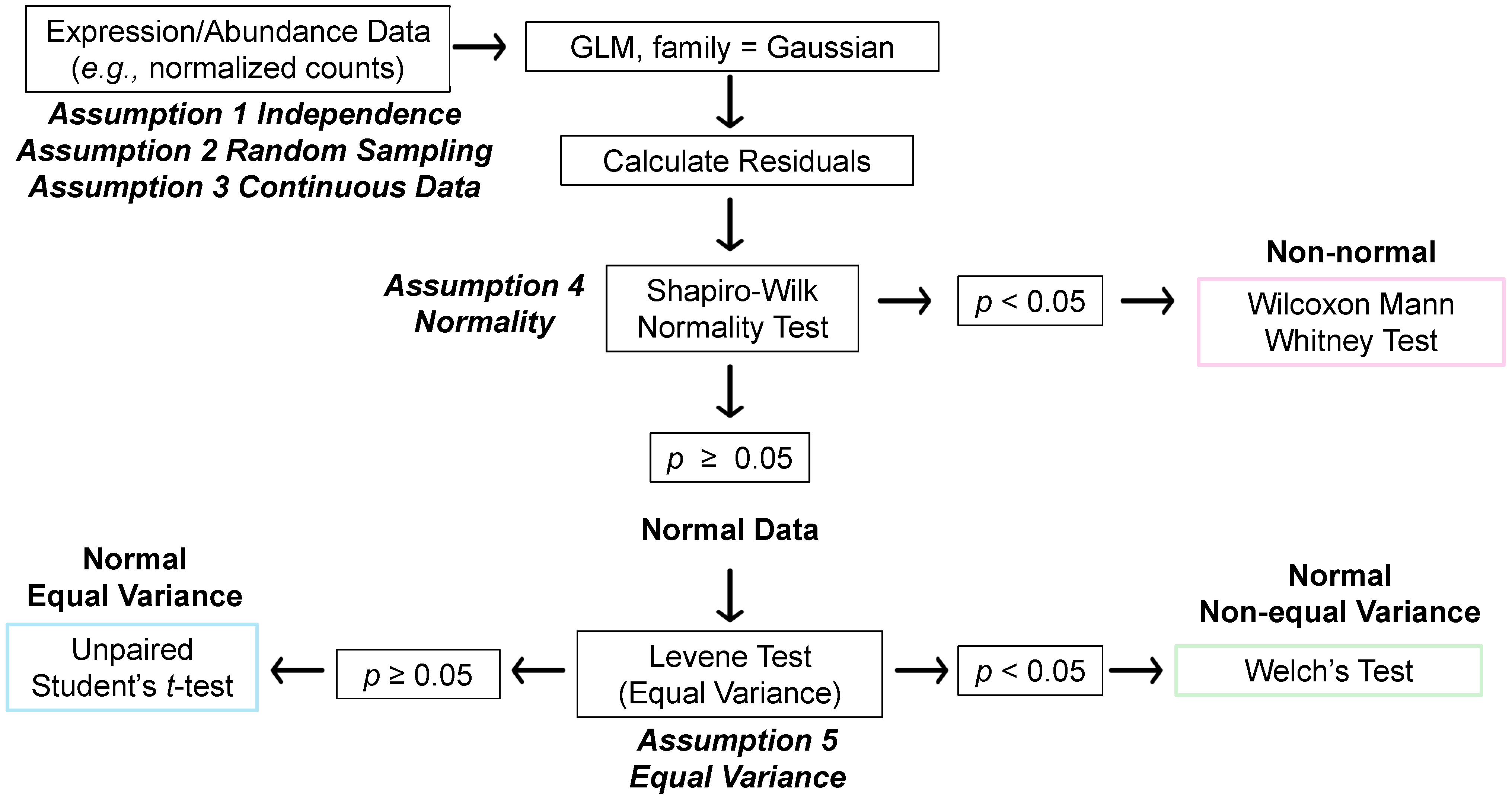
3.1. STATom@ic: Two-Group Statistical Comparisons

In order to use the two-group comparison feature of STATom@ic, data must be from two groups and meet the following assumptions: (1) independence (e.g., data points do not impact the value of other data points), (2) random sampling (e.g., data selected at random), and (3) continuous data. STATom@ic can handle unequal group distributions (e.g., n = 3 vs. n = 4). However, if values for every sample in more than one group are the same or 0, these data should be pre-filtered prior to the use of STATom@ic, as well as missing values. Continuous variable data from two groups that were independent and randomly sampled were used for this STATom@ic pipeline. The residuals were first calculated by a generalized linear model (GLM) [10] (Figure 1). The GLM was used as it can calculate residuals for normal and non-normal data prior to normality testing [10]. Calculated residuals were then used in the Shapiro–Wilk normality test [11] to test for assumption 4, a normal distribution. The Shapiro–Wilk test was used to test for normality as it can be used for smaller sample sizes [12] typically observed in omic datasets. Other normality tests can be substituted if the Shapiro–Wilk test is not preferred. Data that had a p < 0.05 (failed normality test) in the Shapiro–Wilk test were then considered non-normal and were subjected to the Wilcoxon Mann–Whitney test [13]. The Wilcoxon Mann–Whitney test is more commonly used in the biological sciences [14] but it can easily be substituted for another non-parametric test such as the Kolmogorov–Smirnov test if necessary. Normal data (data with a p ≥ 0.05 in the Shapiro–Wilk test, passed normality test) were then used in the Levene test [15] to test for assumption 5, equal group variances. The Levene test was chosen as it is not sensitive to normality [16]. Normal data with a p ≥ 0.05 in the Levene test were considered to have equal variances between groups and were then subjected to the unpaired Student’s t-test [17]. An unpaired Student’s t-test was chosen as it can be used for smaller sample sizes typical of omic data, but other two-group parametric tests can be substituted as needed. Then, normal data that had a p < 0.05 in the Levene test were analyzed via Welch’s test [18] and were considered to have unequal variances. Welch’s test was selected as it is a robust test for normal data with unequal variances [19], but alternative tests can be substituted. The output result file (.csv format) had columns identified as analyte ID (e.g., Gene ID), group means, log₂ Fold-Change, p-value, and the statistical test used. The result file can be modified to show only significant data (e.g., p < 0.05) from all three tests, all data regardless of statistical significance, or three separate result files based on the statistical test used.

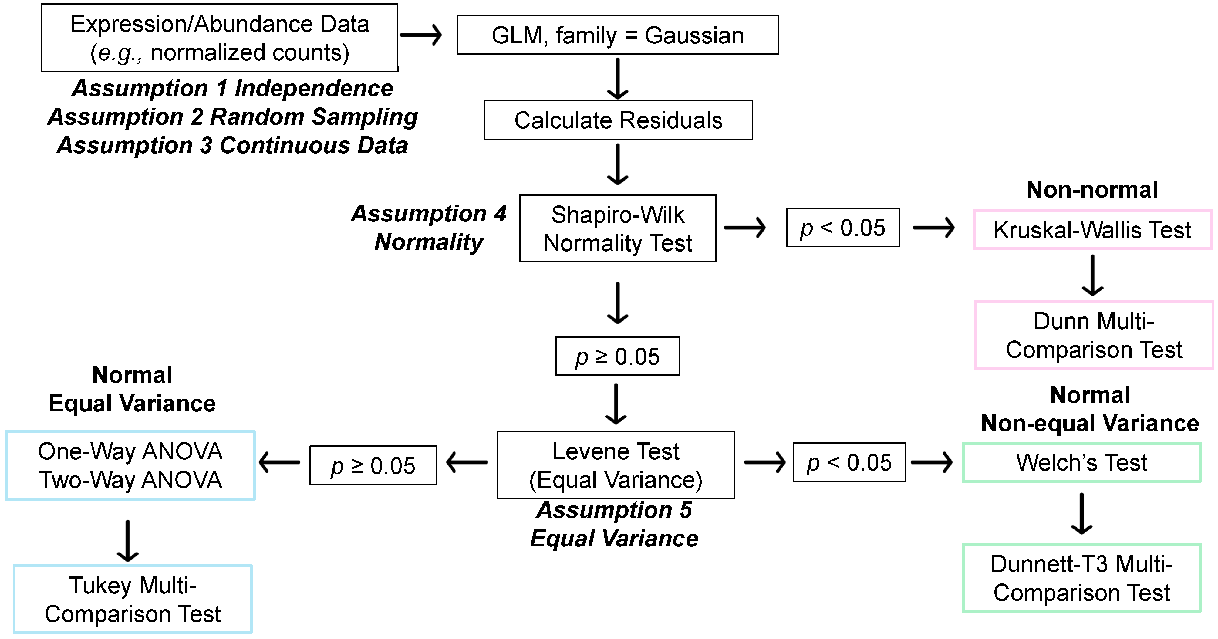
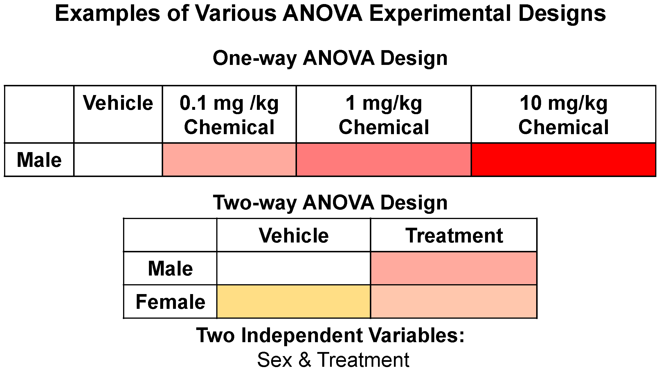
3.2. STATom@ic Multi-Group Statistical Comparisons

The STATom@ic multi-group comparison workflow (Figure 2) includes the option to perform a one- [20] or two-way [21] ANOVA based on the user’s experimental design (Figure 3). If there is not a two-variable experimental design (e.g., sex and treatment), then, most likely, a one-way ANOVA is most appropriate. Like the two-group comparison statistical framework, multi-group data must meet the following assumptions: (1) independence, (2) random sampling, and (3) continuous data. STATom@ic can handle unequal group distributions (e.g., n = 3 vs. n = 4). However, if values for every sample in more than one group are the same or 0, these data should be pre-filtered prior to the use of STATom@ic, as well as any missing values. Similar to the two-group comparison workflow, a generalized linear model (GLM) was used followed by the calculation of the residuals. The residuals were used to test assumption 4, for normality, via the Shapiro–Wilk normality test. An alternative normality test can be used if necessary. Data were deemed non-normal if the Shapiro–Wilk test showed p < 0.05 (failed normality test) and were subjected to the Kruskal–Wallis test [22] with a Dunn multi-comparison test [23]. The Kruskal–Wallis test was selected for its utility for non-parametric data and data with a small sample size [24]. The Dunn multiple comparison test is a useful post hoc test for nonparametric, multi-group data to pinpoint which head-to-head comparisons are significant [23]. Normal data (p ≥ 0.05 in Shapiro–Wilk test, passed normality test) were then used in the Levene test to determine if the variances between groups were equal, which was assumption 5. Normal data with unequal group variances (p < 0.05 by the Levene test, unequal variance) were subjected to Welch’s test and the Dunnett T3 multiple comparison test [25]. Welch’s test was used for normal data with unequal variances followed by the Dunnett T3 post hoc multiple comparison test, which is useful for groups with a small sample size [26]. Other multiple comparison tests can be used as justified by the user data. Next, normal data with equal group variances (p ≥ 0.05 by the Levene test, equal variance) were used in the corresponding one- or two-way ANOVA test based on the experimental design (Figure 3) with the post hoc Tukey multiple comparison test [27]. One-way or two-way ANOVAs were used as they are robust and commonly used in the biological sciences [28]. Other post hoc multiple comparison tests can be used in place of Tukey including Bonferroni or Sidak. STATom@ic can be performed on basic office computers (e.g., Windows or Mac with 8GB of RAM) and takes only a few minutes for data with up to 20,000 rows.

In order to assess STATom@ic capabilities to determine true positives (precision) and limit the detection of false negatives (recall), the same RNASeq data (Supplemental Excel File S1) and respective p-values were analyzed via confusion matrix analysis (

Table 1. Confusion matrix analysis determined that STATom@ic had high precision but low recall compared to DeSeq2.

Confusion Matrix (STATom@ic vs. DeSeq2)
	p < 0.05
True Positive	852
False Negative	2575
False Positive	49
True Negative	10,256
Recall	0.2486
Precision	0.9456

). Using the DeSeq2 output p-values as the reference and the STATom@ic output p-values for comparison, we found that STATom@ic had high precision (0.9456) but low recall (0.2486) compared to DeSeq2.

4. Discussion

Here we describe a novel, modular, and free statistical tool that can be used as a stand-alone or in addition to establish pipelines to analyze continuous variable data. Many statistical tests applied to omic datasets employ a “one size fits all” statistical test that has a set of assumptions that are unmet. While this can be satisfactory for generating a hypothesis, it may not be the best method for analyzing the researcher’s data. STATom@ic uses many statistical tests common to data analysis in the biological sciences but could be useful for other fields of research or analytical fields.

The greatest strengths of the STATom@ic R package are that it (1) applies the appropriate test based on the characteristics of the data without human intervention or bias, (2) does so in a high-throughput manner, and (3) is user-friendly as it requires little to no specialized coding skills to use as is. The automation of STATom@ic prevents users from performing “p-value hacking” or “data dredging” either on purpose or by accident. p-value hacking is where a researcher applies a barrage of statistical tests to their data in search of a significant p-value regardless of whether the test is appropriate for their data. Since STATom@ic performs all of the appropriate statistics, this limits the ability of users to interfere and perform p-value hacking. Having an unbiased tool like STATom@ic will help researchers abide by the NIH’s standards on rigor, reproducibility, and transparency and initiatives such as Big Data to Knowledge [29], among others. Obviously, STATom@ic is useful for omic datasets but it could also be used for other small to midsize datasets as well. While R has been a free and tremendously useful tool for statistical analysis in research, it is often underused by researchers who lack the required skillset or background. Many researchers will opt to pay for statistical software that is easier to use. STATom@ic is used via R and the code and tutorials are freely available, allowing anybody to use the package regardless of their background.

For users who do have more of a coding background, STATom@ic is modular and fully customizable. All the STATom@ic source codes and tutorials are available online at no cost (github.com/ruitreves/statomatic, accessed on 1 January 2025). STATom@ic can be modified to replace statistical tests based on the end user′s needs. For example, the Tukey multiple comparison test could be replaced by a Sidak or Bonferroni test if needed. The output result files can be customized as well to include more or less information.

STATom@ic excels at hypothesis testing that is not based solely on head-to-head comparisons, which is common to certain pipelines that calculate differentially expressed genes, for example [30]. Although STATom@ic can perform multiple-group comparisons or two-group comparisons, it also offers the functionality to perform one-way and two-way ANOVAs. STATom@ic is not intended to replace data analysis pipelines but to be used in combination once a molecule matrix (e.g., gene matrix) is generated. STATom@ic does not curate, map, or identify molecules of interest but performs statistics on gene/protein/metabolite matrices acquired from other pipelines. In addition, STATom@ic can be downloaded and used on very basic office computers (e.g., 8 GB RAM) to analyze relatively large datasets (e.g., gene matrices with up to 50,000 genes) in minutes. To our knowledge, this is the first statistical framework that will automatically perform assumption testing and apply the appropriate statistical test without human interference. We found that STATom@ic has high precision compared to DeSeq2, which means that one of STATom@ic’s strengths is its ability to identify true positives (e.g., significantly differentially expressed genes (DEGs)).

While STATom@ic has many noteworthy strengths, it does have some inherent weaknesses. If there are identical values (e.g., all zeroes) for a molecule of interest for multiple groups, the statistics cannot be performed properly. Thus, data may need to be pre-filtered prior to use in STATom@ic or the user may decide to use a method of imputation for missing values [31]. One other limitation currently is the inability to identify outliers that may be shifting the distribution from normal to non-normal. The end user may decide to remove an outlier for all analytes (e.g., all data tied to a specific sample) and then run it through STATom@ic or use the data as they are based on the user’s discretion. Currently, imputation and outlier identification are not features of STATom@ic but may be offered in the foreseeable future. Since STATom@ic only performs statistics on a previously obtained data matrix, sequencing data will need to be trimmed, mapped, and normalized prior to statistical testing. Since metabolomic and proteomic data are usually provided as a data matrix, these forms of data can be used as they are. While STATom@ic had high precision, it had low recall compared to DeSeq2, indicating that it may be stringent and identify more false negatives (e.g., non-significant DEGs that are actually significant).

We would implore fellow researchers to try STATom@ic (www.github.com/ruitreves/statomatic, accessed on 1 January 2025) on omic data from a past experiment or publicly available data and determine how well it fits their needs compared to other statistical methods. We hope users may find it to be more robust and more streamlined compared to other statistical methods. In fact, we hope users may identify new genes, proteins, or metabolites of interest that were not identified as statistically significant in their previous method but are with STATom@ic.

5. Conclusions

STATom@ic is a novel, free, and rigorous statistical package that can be used to analyze any size dataset in an unbiased manner. Further, this package is fully customizable and modular for the experienced user or can be used as is for the more novice R user. STATom@ic automatically uses the appropriate statistical test based on the characteristics of the data. This R package can help researchers who do not have dedicated statisticians or bioinformatic resources or facilities or those who cannot afford to wait for long periods of time for statistical analysis. We hope that STATom@ic will be incorporated into users’ current data analysis pipelines for unbiased hypothesis testing. To our knowledge, this is the only publicly available statistical package that can take a user’s omic data matrix (e.g., mRNA, protein, metabolite matrix), automatically test all the assumptions, and apply the appropriate statistical test without human interference. The intent of STATom@ic is to take the “guesswork” out of hypothesis testing and enhance the researcher’s ability to perform the appropriate statistical testing on omic datasets, allowing for the identification of more rigorous and reproducible findings.

References

1. Chen, C.; Wang, J.; Pan, D.; Wang, X.; Xu, Y.; Yan, J.; Wang, L.; Yang, X.; Yang, M.; Liu, G.P. Applications of multi-omics analysis in human diseases. MedComm 2023, 4, e315. [Google Scholar] [CrossRef]
2. Ott, A.W.; Sol-Church, K.; Deshpande, G.M.; Knudtson, K.L.; Meyn, S.M.; Mische, S.M.; Taatjes, D.J.; Sturges, M.R.; Gregory, C.W. Rigor, Reproducibility, and Transparency in Shared Research Resources: Follow-Up Survey and Recommendations for Improvements. J. Biomol. Tech. 2022, 33, 3fc1f5fe.fa789303. [Google Scholar] [CrossRef] [PubMed]
3. Williams, J.J.; Drew, J.C.; Galindo-Gonzalez, S.; Robic, S.; Dinsdale, E.; Morgan, W.R.; Triplett, E.W.; Burnette, J.M., 3rd; Donovan, S.S.; Fowlks, E.R.; et al. Barriers to integration of bioinformatics into undergraduate life sciences education: A national study of US life sciences faculty uncover significant barriers to integrating bioinformatics into undergraduate instruction. PLoS ONE 2019, 14, e0224288. [Google Scholar] [CrossRef]
4. Aron, S.; Jongeneel, C.V.; Chauke, P.A.; Chaouch, M.; Kumuthini, J.; Zass, L.; Radouani, F.; Kassim, S.K.; Fadlelmola, F.M.; Mulder, N. Ten simple rules for developing bioinformatics capacity at an academic institution. PLoS Comput. Biol. 2021, 17, e1009592. [Google Scholar] [CrossRef]
5. R Core Team. A Language and Environment for Statistical Computing; Foundation for Statistical Computing: Vienna, Austria, 2020. [Google Scholar]
6. John Fox, S.W. An {R} Companion to Applied Regression; Sage Publications: New York, NY, USA, 2019. [Google Scholar]
7. Dag, O.; Dolgun, A.; Konar, N.M. Onewaytests: An R Package for One-Way Tests in Independent Groups Designs. R J. 2018, 10, 175–199. [Google Scholar] [CrossRef]
8. Dinno, A. Dunn.test: Dunn’s Test of Multiple Comparisons Using Rank Sums. CRAN, 2024. Available online: https://cran.r-project.org/web/packages/dunn.test/dunn.test.pdf (accessed on 1 January 2025).
9. Pohlert, T. PMCMRplus: Calculate Pairwise Multiple Comparisons of Mean Rank Sums Extended_. R Package version 1.9.12. CRAN, 2024. Available online: https://cran.r-project.org/web/packages/PMCMRplus/PMCMRplus.pdf (accessed on 1 January 2025).
10. Nelder, J.A.; Wedderburn, R.W.M. Generalized Linear Models. J. R. Stat. Soc. Ser. A Stat. Soc. 1972, 135, 370–384. [Google Scholar] [CrossRef]
11. Shapiro, S.S.; Wilk, M.B. An analysis of variance test for normality (complete samples). Biometrika 1965, 52, 591–611. [Google Scholar] [CrossRef]
12. Mishra, P.; Pandey, C.M.; Singh, U.; Gupta, A.; Sahu, C.; Keshri, A. Descriptive statistics and normality tests for statistical data. Ann. Card. Anaesth. 2019, 22, 67–72. [Google Scholar] [CrossRef]
13. Wilcoxon, F. Individual Comparisons by Ranking Methods. Biom. Bull. 1945, 1, 80–83. [Google Scholar] [CrossRef]
14. Kühnast, C.; Neuhäuser, M. A note on the use of the non-parametric Wilcoxon-Mann-Whitney test in the analysis of medical studies. Ger. Med. Sci. 2008, 6, Doc02. [Google Scholar] [PubMed]
15. Levene, H. Robust Tests for Equality of Variances. Contrib. Probab. Stat. 1960, 69, 278–292. [Google Scholar]
16. Wang, Y.; Rodríguez de Gil, P.; Chen, Y.H.; Kromrey, J.D.; Kim, E.S.; Pham, T.; Nguyen, D.; Romano, J.L. Comparing the Performance of Approaches for Testing the Homogeneity of Variance Assumption in One-Factor ANOVA Models. Educ. Psychol. Meas. 2017, 77, 305–329. [Google Scholar] [CrossRef] [PubMed]
17. Student. The Probable Error of a Mean. Biometrika 1908, 6, 1–25. [Google Scholar] [CrossRef]
18. Welch, B.L. The Generalization of ‘Student’s’ Problem When Several Different Population Varlances Are Involved. Biometrika 1947, 34, 28–35. [Google Scholar] [CrossRef]
19. Derrick, B.; White, P. Why Welch’s test is Type I error robust. TQMP 2016, 12, 30–38. [Google Scholar] [CrossRef]
20. Fisher, R.A. Studies in crop variation. I. An examination of the yield of dressed grain from Broadbalk. J. Agric. Sci. 1921, 11, 107–135. [Google Scholar] [CrossRef]
21. Fisher, R.A. Statistical Methods for Research Workers. In Breakthroughs in Statistics: Methodology and Distribution; Kotz, S., Johnson, N.L., Eds.; Springer: New York, NY, USA, 1992; pp. 66–70. [Google Scholar]
22. Kruskal, W.H.; Wallis, W.A. Use of Ranks in One-Criterion Variance Analysis. J. Am. Stat. Assoc. 1952, 47, 583–621. [Google Scholar] [CrossRef]
23. Dunn, O.J. Multiple Comparisons Among Means. J. Am. Stat. Assoc. 1961, 56, 52–64. [Google Scholar] [CrossRef]
24. Ostertagová, E.; Ostertag, O.; Kováč, J. Methodology and Application of the Kruskal-Wallis Test. Appl. Mech. Mater. 2014, 611, 115–120. [Google Scholar] [CrossRef]
25. Dunnett, C.W. Pairwise Multiple Comparisons in the Unequal Variance Case. J. Am. Stat. Assoc. 1980, 75, 796–800. [Google Scholar] [CrossRef]
26. Games, P.A.; Keselman, H.J.; Rogan, J.C. Simultaneous pairwise multiple comparison procedures for means when sample sizes are unequal. Psychol. Bull. 1981, 90, 594–598. [Google Scholar] [CrossRef]
27. Tukey, J.W. Comparing Individual Means in the Analysis of Variance. Biometrics 1949, 5, 99–114. [Google Scholar] [CrossRef] [PubMed]
28. Larson, M.G. Analysis of Variance. Circulation 2008, 117, 115–121. [Google Scholar] [CrossRef] [PubMed]
29. Bourne, P.E.; Bonazzi, V.; Dunn, M.; Green, E.D.; Guyer, M.; Komatsoulis, G.; Larkin, J.; Russell, B. The NIH Big Data to Knowledge (BD2K) initiative. J. Am. Med. Inf. Assoc. 2015, 22, 1114. [Google Scholar] [CrossRef] [PubMed]
30. Love, M.I.; Huber, W.; Anders, S. Moderated estimation of fold change and dispersion for RNA-seq data with DESeq2. Genome Biol. 2014, 15, 550. [Google Scholar] [CrossRef]
31. Austin, P.C.; White, I.R.; Lee, D.S.; van Buuren, S. Missing Data in Clinical Research: A Tutorial on Multiple Imputation. Can. J. Cardiol. 2021, 37, 1322–1331. [Google Scholar] [CrossRef] [PubMed]
Figure 1. STATom@ic decision tree for two-group statistical comparisons. In this decision tree, data from two groups was processed in this pipeline for assumption testing prior to the final statistical tests including the Wilcoxon Mann–Whitney test (non-normal data), Welch’s test (normal data with non-equal variance), or unpaired Student’s t-test (normal data with equal variance). GLM: generalized linear model.
Stats 08 00018 g001
Figure 2. STATom@ic multi-group statistical comparisons. In this decision tree, multiple group data were subjected to assumption testing prior to the final statistical tests including the Kruskal–Wallis test with a Dunn multiple comparison post hoc test (non-normal data), Welch’s test with a post hoc Dunnett-T3 multiple comparison test (normal data with non-equal variance), or a one-/two-way ANOVA with a post hoc Tukey multiple comparison test (normal data with equal variance). GLM: generalized linear model.
Stats 08 00018 g002
Figure 3. Example of experimental designs for one- or two-way ANOVAs. Three or more groups of data that do not have overlapping variables are more than likely going to be used for a one-way ANOVA as long as the data are normal with equal variances. Four groups of data with overlapping variables (e.g., sex and treatment) or a 2 × 2 design will be used for a two-way ANOVA as long as the data are normal with equal variances.
Stats 08 00018 g003