Abstract
We propose an unbiased restricted estimator that leverages prior information to enhance estimation efficiency for the linear regression model. The statistical properties of the proposed estimator are rigorously examined, highlighting its superiority over several existing methods. A simulation study is conducted to evaluate the performance of the estimators, and real-world data on total national research and development expenditures by country are analyzed to illustrate the findings. Both the simulation results and real-data analysis demonstrate that the proposed estimator consistently outperforms the alternatives considered in this study.
1. Introduction
Consider the following linear regression model:
where is an vector of the dependent variable of observation, is an matrix of explanatory variables of rank , is a vector of unknown parameters, and is an error vector, which follows a multivariate normal distribution, with and covariance matrix equal to . Also, is the error variance and is the identity matrix of size n.
The ordinary least-squares (OLS) estimator for model (1) can be written as follows:
where . In the linear regression model, the unknown regression coefficients are estimated using the OLS estimator.
The linear regression model in (1) is based on a set of assumptions that determine the process of its use in estimating the relationship between the dependent variable and the explanatory variables. One of these assumptions is the absence of a linear relationship, which is called multicollinearity between the explanatory variables, such that this relationship is not strong or harmful. The presence of a strong relationship between the explanatory variables affects the estimates of the model parameters, which is reflected in the decision-making process to accept or reject the null hypothesis. The reason for this is that the presence of a strong relationship will affect the correlation matrix, which is reflected in its inverse. Thus, the variance of the least-squares estimates will be inflated, which will cause the least-squares method to lose the property of the best-unbiased estimator.
Regularization techniques like Ridge regression or Lasso regression, which add a penalty for high coefficients, are used for helping to mitigate the effects of multicollinearity. However, the ordinary ridge regression (), which, suggested by Hoerl and Kennard (1970), is one of the most famous biased estimators that is used to reduce the effects of multicollinearity problems on estimation [1]. Although the estimator is always biased, it outperforms the OLS estimator by the criterion of sampling variance. However, the sampling variance is not an appropriate criterion for evaluating the performance of a biased estimator. For this reason, Crouse et al. (1995) introduced the unbiased ridge regression () estimator, which is one of the most important estimators and the most popular due to its statistical properties [2]. It aims to reduce the variance. Therefore, the resulting estimator has a lower mean-squared error (MSE) compared to the OLS, as well as to the ORR. Özkale and Kaçiranlar (2007) introduced the unbiased ridge regression (URR) estimator in two different ways and compared their performances with the other estimations [3].
Also, if there is prior information about the unknown parameters or any additional information that helps in the process of estimating those parameters, this will increase the accuracy and performance of the estimator. Therefore, the restricted least-square (RLS) estimator has minimum variance compared to the OLS estimator. Combining two estimators creates a new estimator that inherits beneficial statistical properties from both. Therefore, a convex combination of these estimators can be advantageous when both seem suitable for a particular scenario. The MSE of this convex combination is constrained by the higher MSE of the individual estimators. This motivated us to propose a new unbiased convex estimator for the regression parameters of the linear regression model.
The aim of this article is to obtain an unbiased estimator depending on prior information and a restricted ridge regression estimator proposed by Sarkar (1992) using the convex combination technique [4]. Therefore, we can use it in the applied aspect to avoid the problem of multicollinearity and obtain estimators that are more accurate than existing estimators.
The rest of this paper is organized as follows: In Section 2, the model and the proposed estimator, as well as its statistical properties are provided. In Section 3, the performance of the new estimator compared with other estimators using the mean-squared-error criterion is studied. In Section 4, the results of a Monte Carlo simulation study are provided to support the theoretical results. Finally, a real dataset is studied with some discussions to justify the superiority of the new convex in Section 5. This paper ends with some concluding remarks.
2. The Proposed Convex Estimator
When there is multicollinearity, the OLS estimator will lose the property of the best estimator, as this correlation between the independent variables will cause an inflation of the variance that increases with the strength of the correlation.
For this reason, the ORR is an estimator that comes by minimizing the objective function , where C is a p matrix, with respect to to obtain an estimator that will reduce the inflation of the variance as follows:
For more on ridge regression methods for different models, we refer to Hoerl and Kennard (1970), Månsson et al. (2018), Kibria and Banik (2016), Alheety and Kibria (2011, 2020), and, recently, Kibria (2022), among others [1,5,6,7,8,9]. The was a linear combination of prior information, with the OLS estimator as follows:
where is a random vector with and independent of .
The RLS method enables the use of sample information and prior information simultaneously. The RLS method is not affected by the multicollinearity problem and works to reduce the variance due to prior information about the parameter and the sample. The RLS estimator is obtained by minimizing the subject to the linear restrictions where r is a vector of known elements and R is a full-row rank matrix with known elements. The RLS estimator can be written as follows [10]:
This estimator is unbiased and has a smaller variance than the OLS when the assumed restrictions are true. If the restrictions are incorrect, the reduction in sampling variance still exists, but the estimator becomes a biased one.
The convex estimator can be provided as follows:
where and can be any two estimators, and A is a square matrix. The convex estimators have the ability to take advantage of the properties of the estimators that compose them and have the potential to deal with multicollinearity effectively.
Wu (2014) studied the philosophy of prior information on as follows [11]:
where C represented matrix, is a random variable distributed as normal with mean and a variance–covariance matrix, and V = . He obtained an unbiased estimator by considering the two-parameter estimator proposed by Ozkale and Kaciranlar (2007) [12]. So, the goal of this paper is to present a generalization of Equation (7) by replacing instead of to obtain a new family of unbiased restricted convex estimators.
In fact, the true parameter may have prior information as a vector called J. Also, if we assume the linear restrictions are satisfied with the model, we can suggest the following general form of the convex estimator (CR) as follows:
To study the optimality of , we find the form of the matrix C that makes the MSE matrix (MSEM) of minimum.
For that, the MSEM of is derived as follows:
A minimum value of L will exist when L is a real-valued, convex, and differentiable function. Therefore, by differentiating (9) with respect to and equating to zero, we obtain:
And then,
Therefore,
where and .
So, the proposed new estimator will be:
where . The random variable and we call it the unbiased restricted ridge regression estimator. The CR estimator is unbiased since:
Also, the variance–covariance matrix of URRR is provided as follows:
Since the CR estimator is unbiased, the MSEM of the CR estimator will be the same as the formula in (13).
We can write the as follows
where MM indicates the MSE matrix.
For all matrices H and F, we will write is a matrix that will be nonnegative definite (n.n.d.), while if will be called a positive definite (p.d.).
3. Comparison of Proposed Estimator
To make a comparison between any two estimators, we may need some of the lemmas below:
Lemma 1.
Let and be the two estimators of The estimator is said to be superior to in the sense of the MSEM criterion if
A scalar mean-squared-error valued version of the is provided by
Now, we will compare the URRR estimator with the RLS estimator by providing the following theorem.
3.1. Comparison Between CR and RLS Estimator
Theorem 1.
If the CR estimator is superior to the RLS estimator using the MSE criterion; that is MM (.
Proof.
The MSEM of the RLS estimator is provided as:
□
So, the difference between is provided as:
Since M and are p.d., we can focus on the results of the matrix . Since Z is p.d., there exists an orthogonal matrix P such that , where is the diagonal matrix of the eigenvalues of Z. A diagonal matrix is a square matrix in which all the elements outside the main diagonal are zero.
Therefore,
We observe that for all i = 1, 2, …, p, and the proof is completed. From the above results, we notice that the new estimator is better than the RLS estimator for all values of k.
Now, we will compare the URR estimator with the CR estimator by providing the following theorem.
3.2. Comparison Between URR and CR Estimator
Theorem 2.
If the CR estimator is superior to the URR estimator using the MMSE criterion; that is MM .
Proof.
The MSEM of URR estimator is provided as:
where . □
Therefore,
The matrix W can be written as follows:
So,
This is a positive definite matrix. Therefore, the proof is completed.
4. Simulation Study
For a numerical comparison among the estimators, a simulation study has been conducted in this section. It consists of two parts: simulation technique and simulation result discussion.
4.1. Simulation Technique
The data generation process for the models was conducted according to a widely used method as described below [13,14,15].
where denotes the correlation coefficient between any two explanatory variables, denotes the independent pseudo-random variable obtained from standard normal distribution, and denotes the number of explanatory variables. Moreover, the dependent variable was obtained through the following equation [16].
where is the error term, i.e., .
In the simulation, three different values of explanatory variables, different values of the correlation coefficients between the explanatory variables, , four different values of the sample sizes, , and two different values of the error variance, , were taken. The data generation process of the explanatory variables was conducted with the help of the values determined for and . In this study, we employed the ridge parameter, denoted as k, within a specified range from 0.1 to 0.9. This range was explored in increments of 0.1, allowing for a comprehensive examination of how varying levels of k influence the outcomes of our analysis. The experiment was repeated, times. The analysis was performed using R programming language version 4.4.2.
The following restrictions were set for different predictors.
When p = 3,
When p = 5,
When p = 10,
The average MSEM was calculated based on the following formula over all simulations [17].
where is any of the URR, RLS, CR, ORR, or OLS estimators, is the true parameter, and p is the number of predictors. We assumed β denotes a p × 1 vector where all elements are equal to 1. This can be expressed as:
4.2. Simulation Results Discussion
4.2.1. Performance as a Function of n
Regarding the sample size, we examined 20, 30, 50, and 100 samples in this study. As the sample size increases, the MSE should be decreased. In Table 1, the proposed CR estimator performs relatively well even with a small sample size when the number of predictors is three. However, a high correlation among the predictors (0.90) adds multicollinearity, affecting its performance slightly. As the sample size increases, the CR estimator stabilizes, with reduced MSE compared to the sample size of 20. The extra data help mitigate some of the issues caused by correlation. MSE continues to decrease, reflecting the benefit of more data. The MSE is significantly lower with this larger sample size, demonstrating the robustness of the CR estimator even in the presence of high correlations. With the same predictors, the high correlation (0.95) adds more multicollinearity. With only 20 samples, the CR estimator tends to exhibit a higher MSE, especially when the predictors are highly correlated. While CR still performs relatively well with limited samples compared to other estimators, significant correlations, such as 0.90, among predictors contributing to increased multicollinearity, subsequently raise the MSE. This indicates that with smaller sample sizes, the negative effects of multicollinearity on estimator performance are more pronounced.

Table 1.
Average MSE values of the estimators when p = 3 and 0.50.
As the sample size increases from 20 to 30 or 50, there is a marked reduction in MSE for the CR estimator. The added data provide a stabilizing effect, enhancing the estimator’s resilience to the multicollinearity caused by high correlations. This improvement in MSE at moderate sample sizes underscores that although high predictor correlation remains a challenge, a larger number of samples helps mitigate its impact on the CR estimator’s accuracy.
At a sample size of 100, the CR estimator consistently achieves its lowest MSE values, even under extreme predictor correlations (e.g., 0.99). With larger samples, the CR estimator displays robustness, as the effect of high correlation among predictors on the MSE diminishes. This trend illustrates the advantages of having more data, as the CR estimator effectively reduces the influence of multicollinearity and maintains a low MSE under challenging high-correlation conditions and multiple predictors.
In summary, as the sample size increases, the MSE of the CR estimator decreases significantly, demonstrating its enhanced ability to manage multicollinearity with more data. The findings emphasize the importance of an adequate sample size in minimizing error, particularly in situations with high predictor correlations. This pattern reinforces the reliability and effectiveness of the CR estimator in maintaining low MSE, even in the face of complex multicollinearity challenges.
4.2.2. Performance as a Function of the Number of Predictors, p
The performance of various estimators is significantly influenced by the size of the predictor set. In this context, we present our proposed estimator, denoted as CR, which demonstrates remarkable adaptability and robustness across a diverse array of scenarios.
When the predictor set comprises a small number of variables (p = 3), the CR estimator consistently outperforms its counterparts, particularly in terms of MSE. This advantage can be attributed to its efficacy in addressing multicollinearity, an effect that becomes increasingly pronounced as the sample size increases. In scenarios characterized by larger sample sizes, CR’s capacity to mitigate the adverse impacts of correlated predictors is particularly noteworthy, resulting in lower MSE compared to alternative estimators.
As we extend the number of predictors to five (p = 5), the model’s complexity escalates, typically leading to an increase in MSE, particularly in the context of smaller sample sizes and elevated correlations among predictors. However, despite these complexities, the CR estimator retains a competitive advantage, effectively reducing MSE more efficiently than its peers as the sample size expands, demonstrating its robust performance in managing more intricate models.
The challenges intensify with 10 predictors (p = 10), where the detrimental effects of multicollinearity and an expanded parameter space are exacerbated. In situations marked by high correlation (e.g., 0.95 and 0.99), we observe a notable increase in MSE due to the inherent difficulties in accurate parameter estimation. Nonetheless, the CR estimator exhibits resilience in these challenging conditions. As sample sizes reach 50 or 100, the performance of CR shows marked improvement, underscoring its adaptability in navigating complex interrelationships among multiple predictors.
In summary, the CR estimator distinguishes itself by consistently reducing MSE across varying sizes of predictor sets. Its strengths are particularly evident in scenarios with larger sample sizes and when confronted with the intricacies of multicollinearity, positioning it as a valuable instrument in the realm of statistical modeling.
4.2.3. Performance as a Function of Correlation Coefficients,
The correlation levels among the predictors, specifically 0.50, 0.70, 0.80, 0.90, 0.95, and 0.99, have a significant impact on the performance of the various estimators. This is clearly demonstrated in the analyses presented in Table 1, Table 2, Table 3, Table 4, Table 5, Table 6, Table 7, Table 8, Table 9, Table 10, Table 11, Table 12, Table 13, Table 14, Table 15, Table 16, Table 17 and Table 18. Generally, higher correlation values are associated with an increase in MSE, indicating a decline in estimation accuracy (Table 1, Table 2, Table 3, Table 4, Table 5, Table 6, Table 7, Table 8, Table 9, Table 10, Table 11, Table 12, Table 13, Table 14, Table 15, Table 16, Table 17 and Table 18).
Table 2.
Average MSE values of the estimators when p = 3 and 0.70.
Table 3.
Average MSE values of the estimators when p = 3 and 0.80.
Table 4.
Average MSE values of the estimators when p = 5 and 0.50.
Table 5.
Average MSE values of the estimators when p = 5 and 0.70.
Table 6.
Average MSE values of the estimators when p = 5 and 0.80.
Table 7.
Average MSE values of the estimators when p = 10 and 0.50.
Table 8.
Average MSE values of the estimators when p = 10 and 0.70.
Table 9.
Average MSE values of the estimators when p = 10 and 0.80.
Table 10.
Average MSE values of the estimators when p = 3 and 0.90.
Table 11.
Average MSE values of the estimators when p = 3 and 0.95.
Table 12.
Average MSE values of the estimators when p = 3 and 0.99.
Table 13.
Average MSE values of the estimators when p = 5 and 0.90.
Table 14.
Average MSE values of the estimators when p = 5 and 0.95.
Table 15.
Average MSE values of the estimators when p = 5 and 0.99.
Table 16.
Average MSE values of the estimators when p = 10 and 0.90.
Table 17.
Average MSE values of the estimators when p = 10 and 0.95.
Table 18.
Average MSE values of the estimators when p = 10 and 0.99.
At a correlation level of 0.90, multicollinearity is evident but remains manageable. Notably, the CR estimator consistently demonstrates superior performance, as indicated by its relatively low MSE values, particularly when examining larger sample sizes. In instances where sample sizes are increased, such as 50 or 100, the CR estimator continues to yield reliable estimates despite the prevailing multicollinearity. Conversely, smaller sample sizes (20 and 30) reveal a significant uptick in variability, resulting in less stable estimates.
As correlation levels rise to 0.95, the adverse effects of multicollinearity become increasingly pronounced, leading to a marked escalation in MSE across all estimators. Nevertheless, the CR estimator maintains a competitive advantage; it experiences a comparatively smaller increase in MSE relative to traditional estimators. The detrimental impacts of heightened correlation are especially observable in smaller samples, where the amplified collinearity exacerbates challenges for the estimators. Notably, as sample sizes expand, the CR estimator reveals its robustness by effectively minimizing MSE in comparison with alternative estimators.
At the maximum correlation level of 0.99, the severity of multicollinearity poses significant obstacles to estimation accuracy. All estimators are subject to a pronounced increase in MSE, with the effects being most severe in smaller sample sizes. In these circumstances, the CR estimator displays remarkable resilience, consistently yielding lower MSE values compared to its counterparts. This advantage becomes particularly salient as the sample size approaches 50 or 100, wherein the CR estimator continues to furnish more stable and accurate estimates.
In summary, across all evaluated correlation levels, the CR estimator consistently demonstrates its superiority in navigating scenarios characterized by high correlation. Its capacity to deliver stable and accurate estimates is enhanced with increases in both correlation and sample size, thereby reinforcing its efficacy in environments susceptible to multicollinearity.
4.2.4. Performance as a Function of Error Variance, σ2
When examining the impact of error variance on estimator performance, it is evident that lower error variance (σ² = 1) correlates with improved overall performance of all estimators, aligning with theoretical expectations. In this context, the CR estimator consistently exhibits a reduced MSE relative to traditional estimators across diverse correlations and sample sizes (Table 1, Table 2, Table 3, Table 4, Table 5, Table 6, Table 7, Table 8, Table 9, Table 10, Table 11, Table 12, Table 13, Table 14, Table 15, Table 16, Table 17 and Table 18). Notably, its performance is particularly pronounced in small sample sizes, where CR significantly outperforms conventional estimators such as OLS, especially in high-correlation environments (0.95 and 0.99). This observation underscores the efficacy of the CR estimator in addressing datasets characterized by strong intercorrelations.
As sample sizes increase to 50 or 100, the CR estimator continues to showcase superior performance, effectively maintaining a low MSE despite an increasing number of predictors. This resilience indicates that CR is adept at managing multicollinearity, a prevalent issue when predictors are highly correlated while also exhibiting robustness in the presence of noise, particularly when the error variance remains comparatively low.
Conversely, as the error variance escalates to σ² = 5, the challenges associated with noise become more pronounced, resulting in a general increase in MSE across all estimators (Table 1, Table 2, Table 3, Table 4, Table 5, Table 6, Table 7, Table 8, Table 9, Table 10, Table 11, Table 12, Table 13, Table 14, Table 15, Table 16, Table 17 and Table 18). Nevertheless, the CR estimator retains a significant advantage in minimizing MSE, particularly under conditions of high correlation. The augmentation of noise exacerbates the complications associated with multicollinearity. However, CR remains resilient in such challenging scenarios.
In stark contrast, traditional estimators like OLS experience a pronounced increase in MSE as error variance rises. In larger sample sizes (n = 50 or 100), the CR estimator adeptly controls the MSE escalation, thereby demonstrating its robustness. This capacity to sustain performance amid more challenging error conditions highlights the potential of the CR estimator as a reliable tool in diverse statistical contexts, especially those marked by significant noise and correlation challenges.
In summary, the findings substantiate the effectiveness of the CR estimator in minimizing error and enhancing accuracy, particularly in environments characterized by multicollinearity and varying levels of noise.
5. Application
5.1. Example 1: Gross National Product Data
To substantiate the simulation results of this study, we conducted an analysis of data regarding total national research and development expenditures as a percentage of gross national product by country from 1972 to 1986. These data were referenced by Akdeniz and Erol (2003) and Gruber (1998) to compare several biased estimators (Table 19) [18,19]. The analysis highlights the relationship between the dependent variable , representing the percentage spent by the USA and four independent variables that indicate the percentages spent by France (), West Germany (), Japan (), and the former Soviet Union ().
Table 19.
Total national research and development expenditures by country.
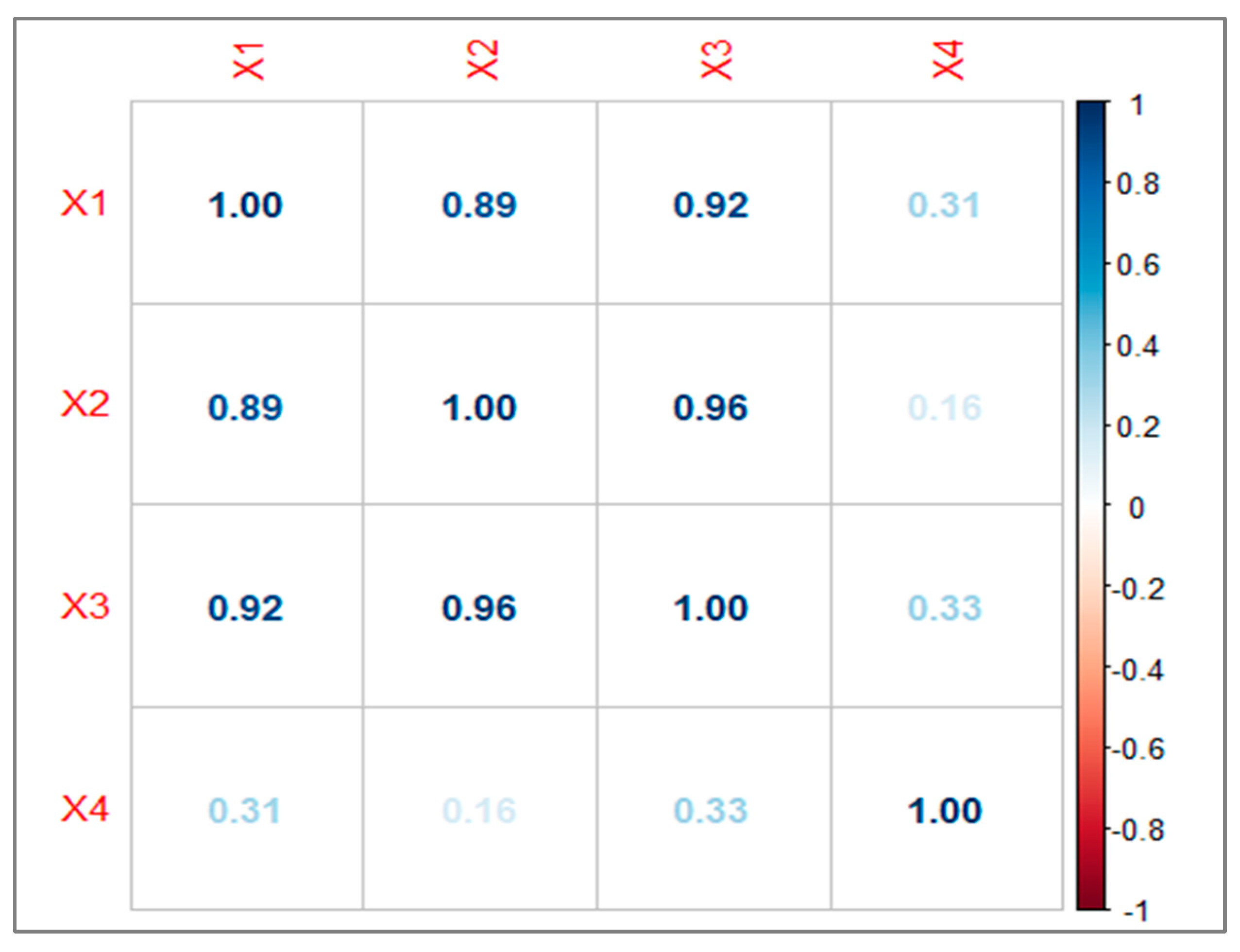
We assessed the multicollinearity within the predictors and discovered that are highly correlated with one another (Figure 1) [20]. Furthermore, the condition number of approximately 74.79 points to the presence of moderate-to-high multicollinearity among the predictor variables. A condition number exceeding 30 indicates significant multicollinearity, which has the potential to distort regression estimates and render the model unstable.
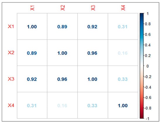
Figure 1.
Correlation matrix.
The following restrictions, and were used, respectively, as follows:
The MSE was computed by evaluating the estimated coefficients of each model against the true coefficients, which was assumed as . For any estimator of , the MSE matrix can be measured by the following:
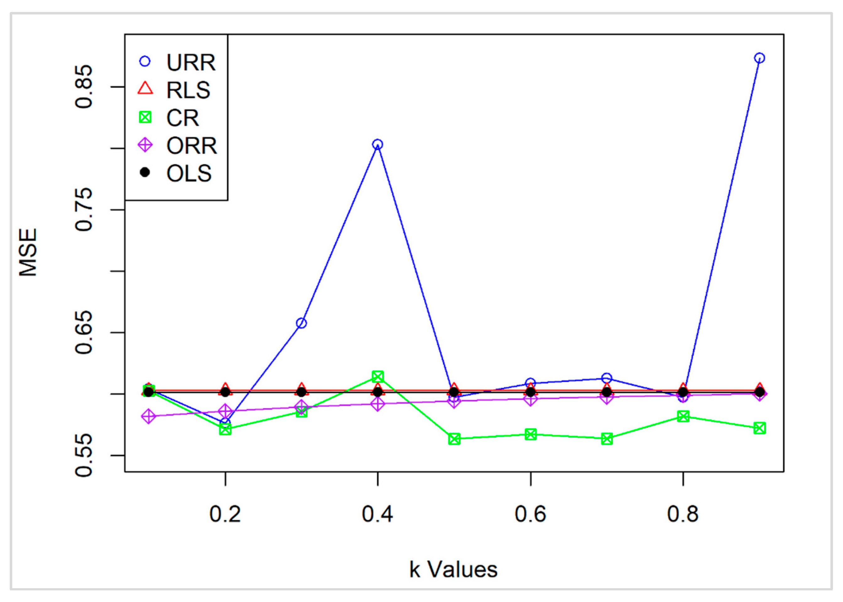
The performance of the proposed CR estimator was evaluated and compared to that of URR, RLS, ORR, and OLS estimators across a range of k values from 0.1 to 0.9, using the aforementioned dataset (Table 20).
Table 20.
MSE of the total national research and development dataset.
The results indicate that CR consistently performs better, achieving lower MSE values than the other estimators. Specifically, CR’s MSE ranges from 0.5637 to 0.6143, with the lowest values recorded at k = 0.5 and k = 0.7 (0.5637 and 0.5639, respectively).
In contrast, URR shows considerable variability, with MSE peaking at 0.8031 for k = 0.4 and 0.8736 for k = 0.9, indicating instability and sensitivity to fluctuations in k. RLS and OLS maintain constant MSE values of 0.6030 and 0.6015, respectively, as they are unrelated to k. However, they fall short in competitiveness compared to CR. While ORR demonstrates moderate performance, it does not achieve lower MSE values than CR in the critical ranges.
These findings highlight CR’s robustness, particularly in the mid-range to close to 1 values of k, emphasizing its potential as a reliable and effective estimator (Figure 2).
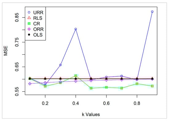
Figure 2.
MSE of the estimators across different k values.
5.2. Example 2: Acetylene Data
Table 21 provides a dataset detailing the percentage conversion of n-heptane to acetylene, alongside three explanatory variables [21]. The condition number of the dataset is calculated to be 93.68234, indicating potential multicollinearity issues. Furthermore, the variance inflation factors (VIFs) for the predictors are VIF₁ = 6.896552, VIF₂ = 21.73913, VIF₃ = 29.41176, and VIF₄ = 1.795332. These values confirm the presence of a significant multicollinearity problem within the dataset. The performance of the estimators, under these conditions, is presented in Table 22.
Table 21.
Acetylene data.
Table 22.
MSE of the estimators for acetylene data.
The performance of the proposed CR estimator was evaluated and compared to that of URR, RLS, ORR, and OLS estimators across a range of k values from 0.1 to 0.9 for this dataset. The results indicate that CR consistently outperforms the other estimators, achieving the lowest MSE values across all the k values. Specifically, CR’s MSE ranges from 0.2782 to 0.9954, with the lowest value observed at k = 0.6 (MSE = 0.2782), demonstrating its superior efficiency in this range. In contrast, URR exhibits extreme variability, with MSE values ranging from 409.9669 at k = 0.1 to 3.0775 at k = 0.9, indicating instability and sensitivity to fluctuations in k. ORR also shows considerable variation, with MSE peaking at 466.8437 at k = 0.1 and gradually decreasing as k increases.
RLS and OLS do not achieve the same level of performance as CR. Overall, these findings reinforce CR’s robustness, highlighting its potential as the most effective and reliable estimator among the ones evaluated.
6. Some Concluding Remarks
This paper introduces an unbiased restricted estimator for linear regression models, leveraging prior information to enhance estimation accuracy. The statistical properties of the proposed estimator are thoroughly examined, highlighting its superiority over several existing alternatives. A comprehensive simulation study evaluates the performance of the estimators under various parametric scenarios. Furthermore, the methodology is applied to a real-world dataset to demonstrate its practical utility. The results from both simulations and the real-data analysis consistently show that the proposed estimator outperforms its counterparts. It is anticipated that the insights presented in this study will be valuable to researchers in the field.
Author Contributions
M.I.A., H.N. and B.M.G.K. have contributed equally. All authors have read and agreed to the published version of the manuscript.
Funding
This research received no external funding.
Institutional Review Board Statement
Not applicable.
Informed Consent Statement
Not applicable.
Data Availability Statement
The original contributions presented in this study are included in the article.
Acknowledgments
Authors are grateful to the reviewers for their constructive comments and suggestions, which helped to improve the quality and presentation greatly.
Conflicts of Interest
The authors declare no conflict of interest.
References
- Hoerl, A.E.; Kennard, R.W. Ridge regression: Biased estimation for non-orthogonal problems. Technometrics 1970, 12, 69–82. [Google Scholar] [CrossRef]
- Crouse, R.H.; Jin, C.; Hanumara, R.C. Unbiased ridge estimation with prior information and ridge trace. Commun. Stat.—Theory Methods 1995, 24, 2341–2354. [Google Scholar] [CrossRef]
- Ozkale, M.R.; Kaciranlar, S. Comparisons of the unbiased ridge estimation to the other estimations. Commun. Stat.-Theory Methods 2007, 36, 707. [Google Scholar] [CrossRef]
- Sarkar, N. A new estimator combining the ridge regression and the restricted least squares method of estimation. Commun. Stat.—Theory Methods 1992, 21, 1987–2000. [Google Scholar] [CrossRef]
- Månsson, K.; Shukur, G.; Kibria, B.M.G. Performance of some ridge regression estimators for the multinomial logit model. Commun. Stat.-Theory Methods 2008, 47, 2795–2804. [Google Scholar] [CrossRef]
- Kibria, B.M.G.; Banik, S. Some ridge regression estimators and their performance. J. Mod. Appl. Stat. Methods 2016, 15, 206–238. [Google Scholar] [CrossRef]
- Alheety, M.I.; Kibria, B.M.G. Choosing ridge Parameters in the Linear regression Model with AR(1) Error: A Comparative Simulation Study. Int. J. Stat. Econ. (IJSE) 2011, 7, 10–26. [Google Scholar]
- Alheety, M.I. New versions of liu-type estimator in weighted and non-weighted mixed regression model. Baghdad Sci. J. 2020, 17, 361–370. [Google Scholar] [CrossRef]
- Kibria, B.M.G. More than hundred (100) estimators for estimating the shrinkage parameter in a linear and generalized linear ridge regression models. J. Econ. Stat. 2022, 2, 233–252. [Google Scholar]
- Özkale, M.R. The relative efficiency of the restricted estimators in linear regression models. J. Appl. Stat. 2014, 41, 998–1027. [Google Scholar] [CrossRef]
- Wu, J. An unbiased two-parameter estimator with prior information in linear regression model. Sci. Word J. 2014, 2014, 206943. [Google Scholar]
- Özkale, M.R.; Kaciranlar, S. The restricted and unrestricted two-parameter estimators. Commun. Stat.—Theory Methods 2007, 36, 2707–2725. [Google Scholar] [CrossRef]
- Kibria, B.M.G. Performance of Some New Ridge Regression Estimators. Commun. Stat.-Simul. Comput. 2003, 32, 419–435. [Google Scholar] [CrossRef]
- Alheety, M.I.; Gore, S.D. A new estimator in multiple linear regression model. Model Assist. Stat. Appl. 2008, 3, 187–200. [Google Scholar] [CrossRef]
- Nayem, H.M.; Kibria, B.M.G. A simulation study on some confidence Intervals for Estimating the Population Mean Under Asymmetric and Symmetric Distribution Conditions. J. Stat. Appl. Probab. Lett. 2024, 11, 123–144. [Google Scholar]
- Nayem, H.M.; Aziz, S.; Kibria, B.M.G. Comparison among Ordinary Least Squares, Ridge, Lasso, and Elastic Net Estimators in the Presence of Outliers: Simulation and Application. Int. J. Stat. Sci. 2024, 24, 25–48. [Google Scholar] [CrossRef]
- Najarian, S.; Arashi, M.; Kibria, B.G. A simulation study on some restricted ridge regression estimators. Commun. Stat.-Simul. Comput. 2012, 42, 871–890. [Google Scholar] [CrossRef]
- Akdeniz, F.; Erol, H. Mean squared error matrix comparisons of some biased estimators in linear regression. Commun. Stat.—Theory Methods 2003, 32, 2389–2413. [Google Scholar] [CrossRef]
- Gruber, M.H.J. Improving Efficiency by Shrinkage; Marcel Dekker: New York, NY, USA, 1998. [Google Scholar]
- Kasubi, F.; Mdimi, O.; Nayem, H.M.; Mwambeleko, E.; Shita, H.; Venkata, S.S.G. Deciphering Seasonal Weather Impacts on Crash Severity: A Machine Learning Approach. Inst. Transp. Eng. ITE J. 2024, 94, 39–46. [Google Scholar]
- Marquardt, D.W.; Snee, R.D. Ridge Regression in Practice. Am. Stat. 1975, 29, 3–20. [Google Scholar] [CrossRef]
Disclaimer/Publisher’s Note: The statements, opinions and data contained in all publications are solely those of the individual author(s) and contributor(s) and not of MDPI and/or the editor(s). MDPI and/or the editor(s) disclaim responsibility for any injury to people or property resulting from any ideas, methods, instructions or products referred to in the content. |
© 2025 by the authors. Licensee MDPI, Basel, Switzerland. This article is an open access article distributed under the terms and conditions of the Creative Commons Attribution (CC BY) license (https://creativecommons.org/licenses/by/4.0/).