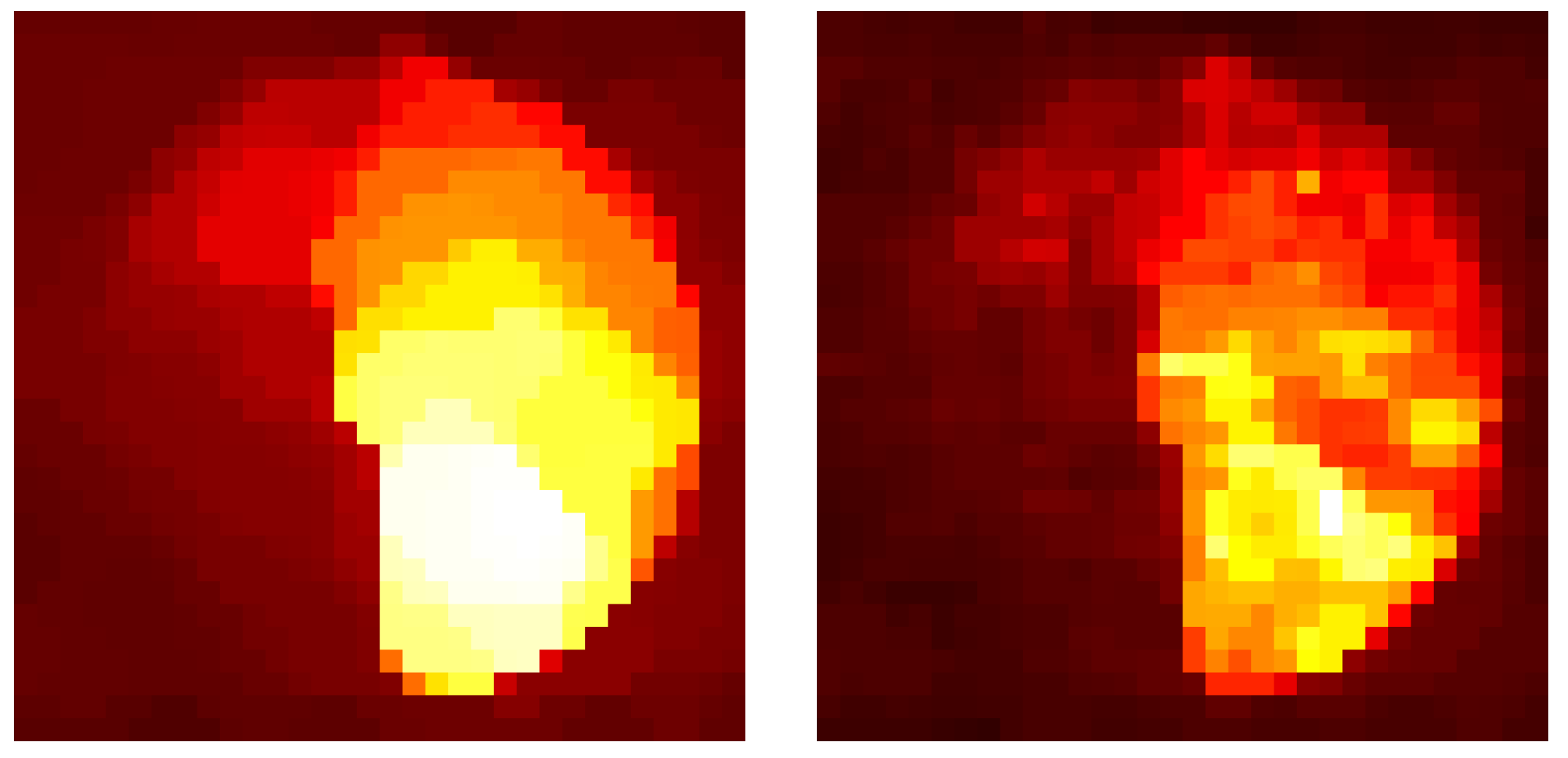
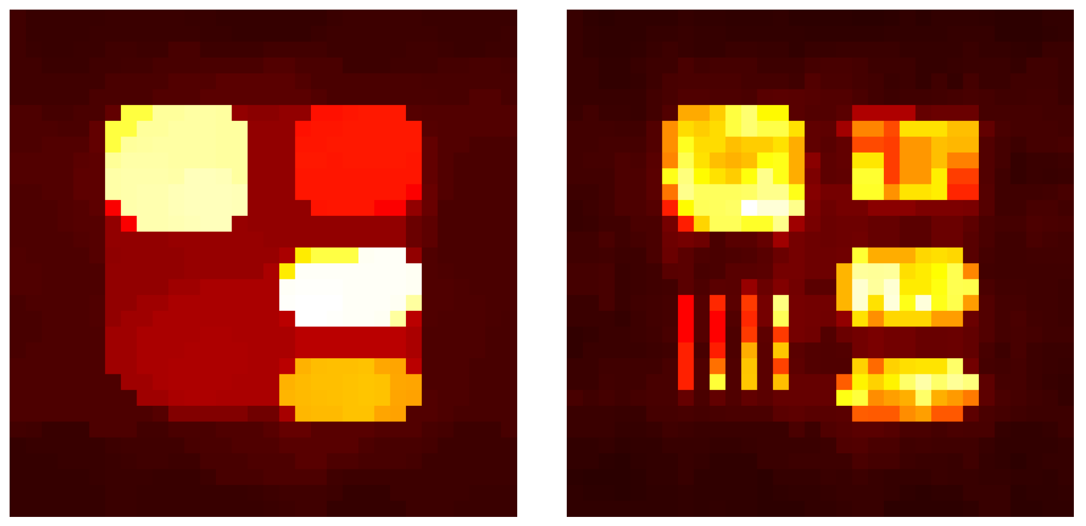
Article

Maximum Penalized-Likelihood Structured Covariance Estimation for Imaging Extended Objects, with Application to Radio Astronomy

School of Electrical and Computer Engineering, Georgia Institute of Technology, 777 Atlantic Drive, Atlanta, GA 30332, USA
Stats 2024, 7(4), 1496-1512; https://doi.org/10.3390/stats7040088
Submission received: 14 November 2024 / Revised: 5 December 2024 / Accepted: 11 December 2024 / Published: 17 December 2024
(This article belongs to the Section Computational Statistics)

Abstract

:
Image formation in radio astronomy is often posed as a problem of constructing a nonnegative function from sparse samples of its Fourier transform. We explore an alternative approach that reformulates the problem in terms of estimating the entries of a diagonal covariance matrix from Gaussian data. Maximum-likelihood estimates of the covariance cannot be readily computed analytically; hence, we investigate an iterative algorithm originally proposed by Snyder, O’Sullivan, and Miller in the context of radar imaging. The resulting maximum-likelihood estimates tend to be unacceptably rough due to the ill-posed nature of the maximum-likelihood estimation of functions from limited data, so some kind of regularization is needed. We explore penalized likelihoods based on entropy functionals, a roughness penalty proposed by Silverman, and an information-theoretic formulation of Good’s roughness penalty crafted by O’Sullivan. We also investigate algorithm variations that perform a generic smoothing step at each iteration. The results illustrate that tuning parameters allow for a tradeoff between the noise and blurriness of the reconstruction.

1. Introduction

The insatiable thirst of astronomers for increasingly high-resolution images of the cosmos has led to ingenious developments in both instrumentation and the processes employed to extract information from the available raw data. In optical astronomy, system resolution is, at first glance, limited by atmospheric turbulence. Undaunted, researchers have tackled challenges with a variety of tactics, including flexible mirrors that can rapidly bend to compensate for the fluctuating atmosphere, and sophisticated signal processing algorithms for combining multiple short exposures into a single image. At the comparatively low frequencies of interest in radio astronomy, the resolution of a single radio telescope is significantly limited by the difficulty and extraordinary cost involved in constructing antennas with large dishes. In the 1940s, this hurdle was overcome by correlating the signals from multiple antennas to form an interferometer. Diverse data can be collected by mounting the antennas on tracks or exploiting the rotation of the earth to take interferometric measurements at different positions [1,2].
The literature on radio astronomy is vast and rich. We have found the collections of papers edited by Goldsmith [3] and Felli and Spencer [4], as well as the text by Thompson, Moran, and Swenson [5], to be particularly helpful. Since the genesis of interferometric radio astronomy, researchers have exploited the connection between the correlation measurements and the Fourier transform of the object being imaged. Basically, each correlation measurement gives an estimate of one point of that Fourier transform. The position of the point in Fourier space depends on the vector separation of the two antennas associated with that measurement. For instance, an array of 27 elements (unequally spaced to avoid redundant position differences) provides 27 2 = 729 Fourier points. In changing the position of the array elements (either by physically moving the elements or by waiting for the Earth to rotate), additional points may be obtained, but it is almost impossible to obtain all the points needed to form a good image by direct Fourier inversion. Simply setting the missing points to zero and applying an inverse Fourier transform yields a blurry image with complicated sidelobe structures, often called a “dirty map”. In addition, negative pixel values are often obtained, even though the intensity should be nonnegative. Radio astronomers have relied on two main tools, the CLEAN algorithm [6,7,8] and maximum entropy [9,10], to produce useful “clean maps”. Although the underlying mapping between the correlation data and the intensity map is linear, the CLEAN and maximum entropy algorithms are both nonlinear forms of processing.
This paper explores a radically different approach based on statistical estimation theory. It does not require or explicitly exploit the Fourier relationships that have dominated radio interferometry for the past fifty years. The method can deal with any reasonable linear relationship between the astronomical source and the raw measurements; the fact that these relationships are complex exponentials is somewhat incidental. Under the statistical model, the pixels that form the sky emit white Gaussian processes. The antenna elements see a mixture of these processes through a linear transformation and additive receiver noise. The signals seen at the antenna elements are then another set of Gaussian process, with correlations between the components. One can then write down the likelihood of the data given unknown powers and maximize the likelihood with respect to unknown parameters. This turns out to be a challenging maximization that does not yield to a frontal assault; hence, we adopt an expectation–maximization (EM) algorithm originally proposed by Snyder, O’Sullivan, and Miller [11] in the different but related context of imaging diffuse radar targets. This is the approach taken by Knapp et al. for radio astronomical imaging using vector sensors in [12].
The CLEAN algorithm requires the astronomer to choose a variety of parameters; the results of this algorithm are often highly dependent on the skill of the practitioner in choosing these parameters. By contrast, in adopting the maximum-likelihood framework, one can “turn the crank” of the EM algorithm without having to tune any such operational parameters. Our approach also fully exploits all statistical knowledge about the data collection.
One of the advantages of maximum-entropy techniques in traditional radio astronomy formulations is that the entropy functional ensures nonnegative estimates. Our approach, which is congruent with that in [12], has this same advantage; nonnegativity is automatically guaranteed by the form of the EM iterations.
To our knowledge, Leshem and van der Veen [13], along with their colleague Boonstra [14], presented the earliest reported work on a maximum-likelihood approach to radio astronomy. They consider imaging in the presence of strong human-made radio interference, for instance, from communication satellites; hence, their primary interest lies in performing maximum-likelihood inference for specific point sources. This yields close ties to the direction-of-arrival literature [15]. They present a simplifying approximation to the log-likelihood and a coordinate descent algorithm that treats already discovered point sources as colored noise. This differs, in both goal and execution, from our EM algorithm for pixel-based imaging. In [16], a maximum-likelihood approach was used to remove unwanted radio sources.
Our work is closer in spirit to that of the pioneering research of Mhiri et al. [17] and Zawadzki et al. [18], which also employed maximum-likelihood estimation for pixel-based imaging. Our work differs fundamentally in that we treat the radiation from each sky pixel as a random process and estimate the parameters of those processes, instead of treating the radiation as a nonrandom parameter. In drawing an analogy with maximum-likelihhood narrowband direction finding, Refs. [17,18] may be thought of as analogous with the “deterministic signal model” of Section III.A in [19], and our work may be thought of as analogous with the “random signal model” of Section III.B in [19].
We employ a Gaussian model for additive noise, whereas [17] employed a compound model consisting of a Gaussian random variable multiplied by an inverse gamma random variable. The algorithms we describe, including various forms of regulation, ensure nonnegative solutions, so an explicit nonnegativity constraint (as described in the last paragraph of Section 4.1 in [17]) is not required. Each iteration of our unconstrained algorithm may be expressed in closed form, unlike Equations (11) and (19) in [17].
Section 2 presents our statistical formulation of the radio astronomy problem, and Section 3 presents the EM algorithm for computing estimates using this model, as well as some simulation results. These experiments illustrate the need for regularization; various possibilities are explored in Section 4. Section 5 suggests some avenues for future exploration.

2. Problem Formulation

Suppose that the sensor array has K elements. Since radio astronomy antennas are quite expensive, it is common to either mount the antennas on tracks, which allow them to be moved, or to simply let the earth rotate, which places them at a new effective look position. Suppose we take data at M such look positions and we collect N snapshots at each position.
Anticipating discretization for computer implementation, we suppose that the sky is made up of I pixels. We will use a single index i = 1 , , I to go over the the entire two-dimensional pixel array. Let ϕ i and θ i denote the angles that pixel i forms with respect to a line perpendicular to and crossing the center of the array. Assume each pixel i radiates a white, complex, zero-mean Gaussian process c i ( n , m ) , n = 1 , , N , m = 1 , , M with unknown variance σ i 2 . Let σ 2 = [ σ 1 2 , , σ I 2 ] T and Σ = diag ( σ 2 ) .
If ϕ i and θ i are small so that small-angle approximations to trigonometric functions apply, each sensor sees the signal from c i with an associated phase shift exp { j 2 π [ x k ( m ) ϕ i + y k ( m ) θ i ] } , where ( x k ( m ) , y k ( m ) ) are the coordinates of sensor k at look position m (see pp. 6–24 of [20]). We can write the data received at sensor k as
r k ( n , m ) = i = 1 I c i ( n , m ) exp { j 2 π [ x k ( m ) ϕ i + y k ( m ) θ i ] } + w k ( n , m ) ,
where w k ( n , m ) is white, complex, zero-mean Gaussian receiver noise with variance N 0 .
Let r = [ r 1 , , r K ] T . For convenience, we form matrices of complex exponentials Γ H ( m ) , m = 1 , , M , and express (1) for all k as
r ( n , m ) = Γ H ( m ) c ( n , m ) + w ( n , m ) ,
where c = [ c 1 , , c I ] T and w = [ w 1 , , w K ] T are independent and identically distributed as C N ( 0 , Σ ) and C N ( 0 , N 0 I ) , independent with respect to each other, and independent with respect to n and m. This is analogous to Equation (13) in [12].
Note that for all n, r ( n , m ) N ( 0 , K r ( m ) ) , where
K r ( m ) = Γ H ( m ) Σ Γ ( m ) + N 0 I .
Estimating the intensity map Σ brings us to the structured covariance estimation waters first charted by Burg et al. [21]. The log-likelihood for the data is
L i d ( Σ ) = N m = 1 M ln det K r ( m ) m = 1 M n = 1 N r H ( n , m ) K r 1 ( m ) r ( n , m ) .

3. An Algorithm for Maximum-Likelihood Imaging

Maximum-likelihood imaging requires us to find the diagonal Σ = d i a g ( σ 2 ) that maximizes (4). Since no simple solution is evident for this difficult optimization problem, we turn to the expectation–maximization algorithm. The algorithm explored here is a trivial extension of the EM algorithm designed by Snyder, O’Sullivan, and Miller [11] in the context of radar imaging. It is similar to formulations presented in [12,22,23,24,25,26,27] and Chapter 6 of the PhD thesis by Robey [28]. In the context of this EM algorithm [29], r ( n , m ) is called the incomplete data, and (4) is the incomplete data log-likelihood.
To formulate an EM algorithm, one postulates a set of complete data that, if available, would make the maximization problem tractable. Here, we take the complete data to be { c ( n , m ) , w ( n , m ) , n = 1 , , N , m = 1 , , M } , where c ( n , m ) C N ( 0 , Σ ) and w ( n , m ) C N ( 0 , N 0 I ) . The classic EM formulation requires that there be a many-to-one mapping from the complete data to the incomplete data; this is provided by (2). The complete data log-likelihood is
L c d ( Σ ) = N M ln det Σ m = 1 M n = 1 N c H ( n , m ) Σ 1 c ( n , m ) = N M i = 1 I ln σ i 2 m = 1 M n = 1 N i = 1 I | c i ( n , m ) | 2 σ i 2 .
Let Q denote the expectation of the complete data log-likelihood given the incomplete data and the estimate from the previous iteration:
Q [ Σ | Σ ( o l d ) ] = df E [ L c d ( Σ ) | Σ ( o l d ) , r ] = N M i = 1 I ln σ i 2 N m = 1 M i = 1 I E [ | c i ( m ) | 2 | Σ ( o l d ) , r ] σ i 2 .
Notice that in the second term, since the N snapshots of c i are independent, we have not notated the explicit dependence of c i on n in the expectation.
At each iteration of the EM algorithm, we obtain the new estimate by maximizing Q:
Σ ( n e w ) = arg max Σ Q [ Σ | Σ ( o l d ) ] .
The derivative of (6) with respect to σ i 2 , set to zero, is
N M 1 σ i 2 + N m = 1 M E [ | c i ( m ) | 2 | Σ ( o l d ) , r ] ( σ i 2 ) 2 = 0 ,
which yields the simple update
σ i 2 ( n e w ) = 1 M E [ | c i ( m ) | 2 | Σ ( o l d ) , r ] .
Computing the expectation in (9) is a standard problem addressed in estimation theory texts (see, for instance, Equation (7.112) on p. 303 of Scharf [30] or Equations (V.B.21) and (7.B.22) on p. 221 of Poor [31]). Its solution results in the explicit update
σ i 2 ( n e w ) = σ i 2 ( o l d ) [ σ i 2 ( o l d ) ] 2 M m = 1 M [ Γ ( m ) K 1 ( m ) Γ H ( m ) Γ ( m ) K 1 ( m ) S ( m ) K 1 ( m ) Γ H ] i i ,
where
K ( m ) = Γ H ( m ) Σ ( o l d ) Γ ( m ) + N 0 I
and
S ( m ) = 1 N n = 1 N r ( n , m ) r H ( n , m ) .
Notice that the data only enter into the inference via its empirical covariance S . We write (10) in a way to show the symmetric structure of the matrix computations. In implementation, it is more efficient to compute the terms in the square brackets of (10) by calculating Ξ ( m ) = Γ ( m ) K 1 ( m ) followed by Ξ ( m ) [ Γ H ( m ) S ( m ) Ξ H ( m ) ] . Since only the diagonal terms are needed, the final step only requires I inner products.
Taking N = 1 in (12) and M = 1 in (10) yields the original algorithm [11] for forming radar images of diffuse targets. In [11], c is the reflectance of a radar scatterer, σ 2 is called its scattering function, and Γ contains time-shifted and doppler-shifted versions of the transmitted waveform.

Simulations

Our simulations were meant to illustrate the overall operation of the EM algorithm, and were not intended to represent any particular real-world scenario. We assumed a 27-element array modeled after the Very Large Array (VLA) in New Mexico [32]. We chose the VLA for this example because it is well known, but the ideas in this paper could be applied to other array geometries. The array consists of three arms arranged in a Y pattern, with equal angular spacing between each arm. Each arm has nine elements. The distance of the nth antenna on each arm from the center of the array is proportional to n 1.716 . The real VLA’s elements are mounted on tracks, so the overall size of the array can be changed. Here, we assume that the array was set at its largest configuration, in which the furthest elements on each arm are 21 km away from the center.
For simplicity, our simulated array departs from the real array in New Mexico in that we supposed the array can be rotated around its center to obtain different looks (or equivalently, the array is centered at one of the Earth’s poles). We supposed that M = 5 different looks were taken, and that the array rotated 10 degrees between looks, for a total rotation of 40 degrees. Figure 1 shows the Fourier sampling pattern this generates in the traditional radio astronomy paradigm. At each look m, N = 500 snapshots were taken to form the empirical covariance matrix S ( m ) . Computations for all results in this paper were performed with MATLAB.
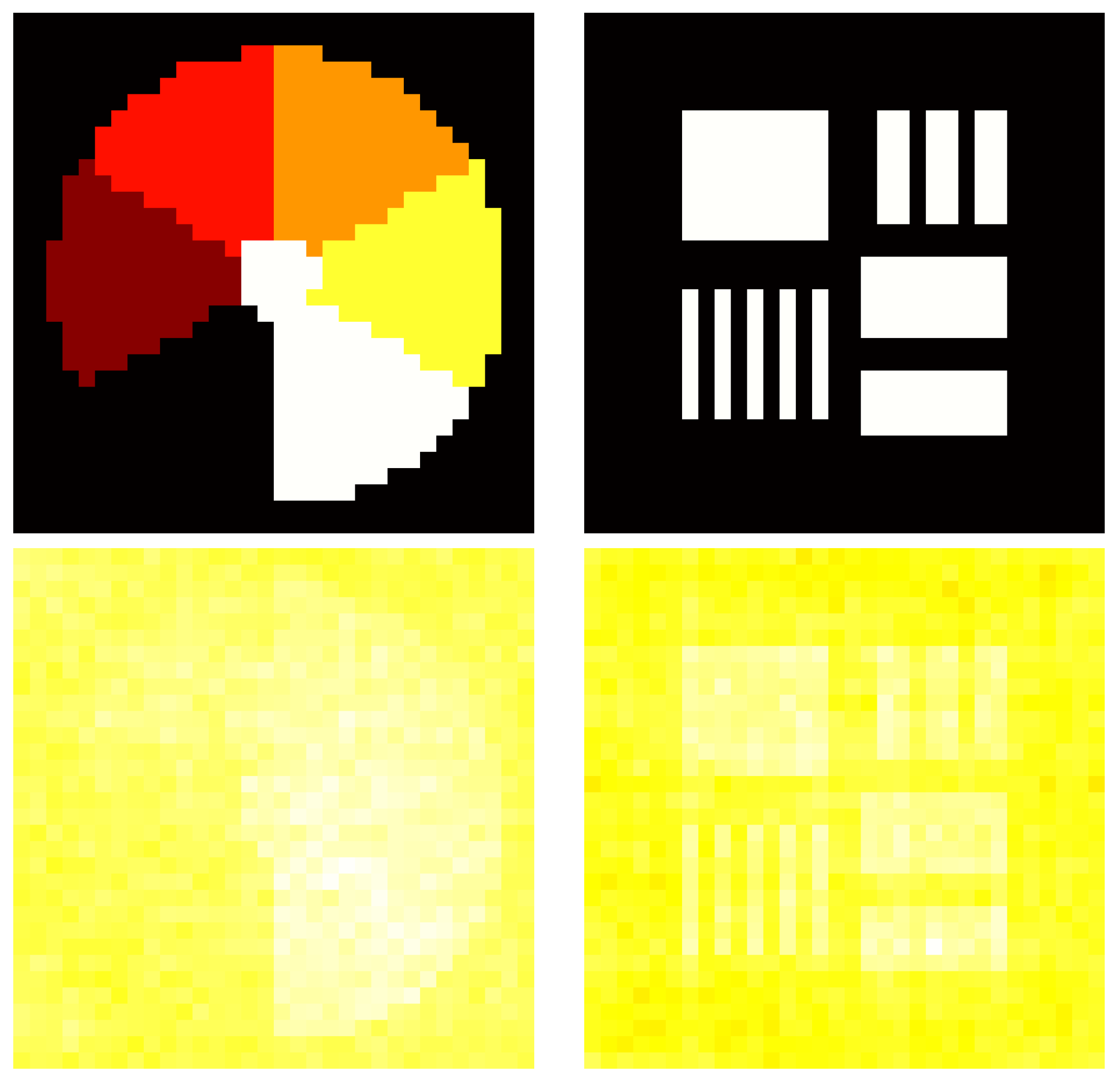
The top row of Figure 2 shows two ideal intensity functions used in our experiments. The bottom row shows the simple estimate
σ ^ i 2 = real m = 1 M Γ ( m ) S ( m ) Γ H ( m ) i i ,
which corresponds to the “dirty map” of traditional radio astronomy.
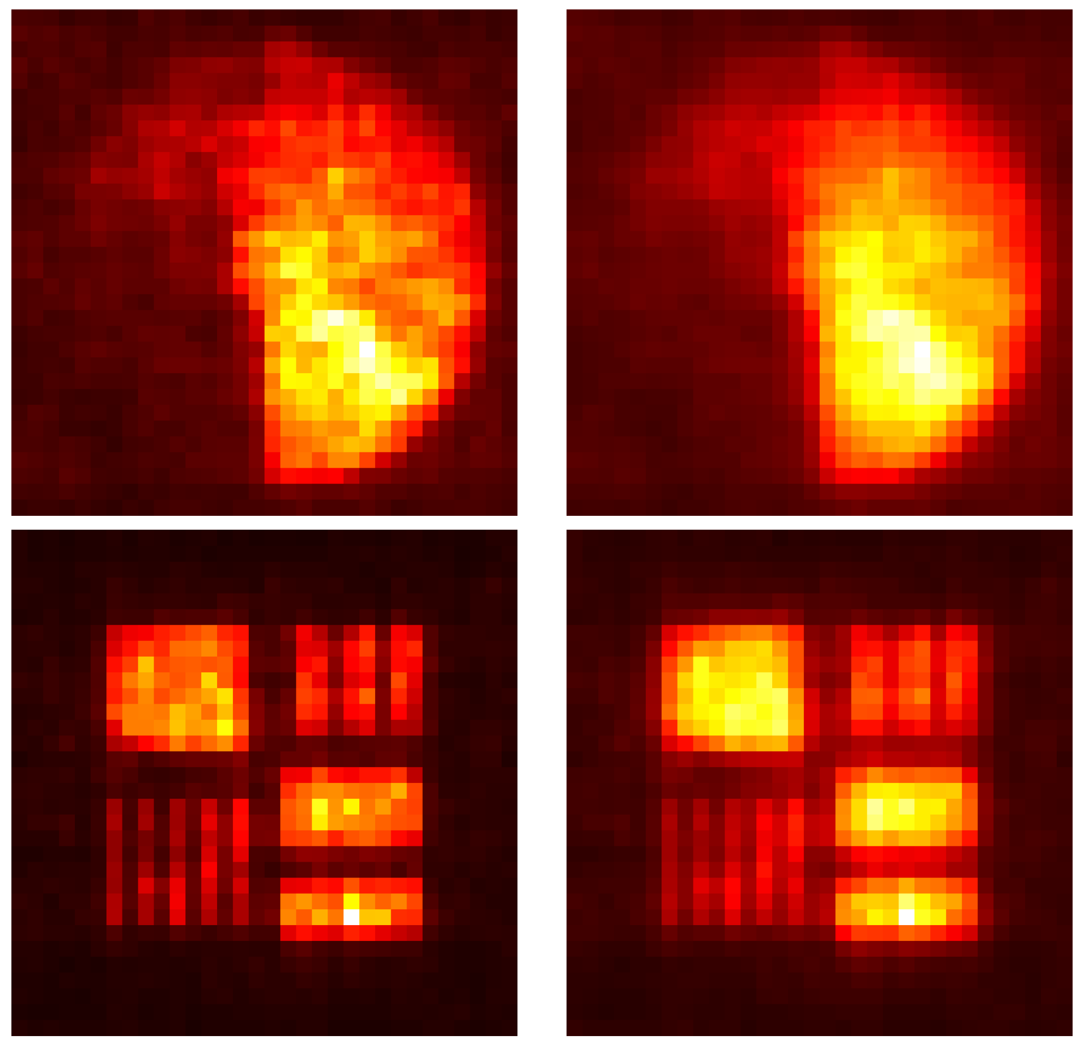
Figure 3 shows the results of EM iterations (10) on data simulated from these ideal intensity functions using the described setup, initialized with a uniform image. Although the results of the EM algorithm do not appear qualitatively much different than the dirty maps in terms of contrast, we see background artifacts being substantially reduced with further iterations.

4. Regularization Techniques

Although the estimates shown in Figure 3 are quite sharp, and the background chaff becomes less evident with increasing iterations, the reconstructed objects suffer from a spiky, noisy appearance. The roughness associated with increasing EM iterations is indicative of the ill-posed nature of the maximum-likelihood estimation of functions from limited data. In most numerical algorithms, accuracy improves as the discretization is refined. Here, the opposite is true; as the grid is refined, the problem becomes increasingly ill posed and the solutions increasingly ill behaved. This phenomenon, called dimensional instability by Tapia and Thompson [33], would manifest itself in any algorithm that maximizes the log-likelihood.
These issues have been extensively studied in the context of Poisson intensity estimation in applications such as medical imaging (see [34,35], and Chapter 3 in [36]). We propose adapting solutions previously applied to Poisson imaging to our radio astronomy problem. The methods explored in this paper are most appropriate for extended objects that do not consist of isolated point sources, such as galaxies and nebula; the need for such methods is outlined in the last paragraph of Section 4 in [12]. For fields of isolated stars, L1-norm regularization, as used in [17], may be more appropriate.

4.1. The Method of Sieves

One approach is to restrict the solution to lie in a restricted subset called a sieve [37]. One possibility is to require it to be a weighted sum of basis functions. Gaussian basis functions have been successful in emission tomography [35,38,39]. In the radio astronomy problem and the related radar imaging problem originally considered by Snyder, O’Sullivan, and Miller [11], the EM algorithm of Section 3 can be extended to incorporate such a sieve constraint. Moulin and co-workers [40,41] presented this extended algorithm (for N = 1, M = 1), along with specific examples employing B-splines for radar imaging. Radio astronomers employing the CLEAN algorithm typically smooth the result by convolving it with a so-called “clean beam”. This clean beam may provide a natural starting point for choosing the sieve in maximum-likelihood estimation. Wavelet thresholding techniques have also been explored for denoising speckled radar imagery [42]. We mention these possibilities for completeness but will not consider them further here.

4.2. Regularization via Penalties

Another approach to regularization is to subtract a penalty Φ ( Σ ) , which discourages unacceptably rough estimates, and to maximize the penalized likelihood
P ( Σ ) = L i d ( Σ ) α Φ ( Σ ) .
Bayesians may think of this as maximum-posterior estimation using a (usually improper) prior proportional to exp [ α Φ ( Σ ) ] .
The EM algorithm can be easily extended to maximize this penalized likelihood. The function Q (6) is generalized to
Q P [ Σ | Σ ( o l d ) ] = df E [ L c d ( Σ ) | Σ ( o l d ) , r ] α Φ ( Σ ) = N M i = 1 I ln σ i 2 N m = 1 M i = 1 I E [ | c i ( m ) | 2 | Σ ( o l d ) , r ] σ i 2 α Φ ( Σ ) .
To maximize (15), we can take derivatives (analogous to (8)) and solve the set of equations
N M 1 σ i 2 + N m = 1 M E [ | c i ( m ) | 2 | Σ ( o l d ) , r ] ( σ i 2 ) 2 α Φ ( Σ ) σ i 2 = 0 ,
alternatively written as
1 σ i 2 + σ i 2 ( u c ) ( Σ ( o l d ) ) ( σ i 2 ) 2 α N M Φ ( Σ ) σ i 2 = 0 ,
where σ 2 ( u c ) ( Σ ( o l d ) ) is the result of the unconstrained update specified by (10). At each iteration, we take the updated value Σ ( n e w ) to be the Σ that solves (17).

4.2.1. Entropy Functionals

Beginning with Frieden [43], numerous authors [44,45,46,47,48,49,50,51,52,53,54] have proposed regularizing a variety of inverse problems with nonnegativity constraints via the entropy functional
Φ E ( Σ ) = i σ i 2 ln σ i 2 .
At each iteration, the new Σ is found by finding the zero of
σ i 2 + σ i 2 ( u c ) ( Σ ( o l d ) ) α N M ( σ i 2 ) 2 ( 1 + ln σ i 2 )
for each i. This is convenient because the solution is decoupled from pixel to pixel. Molina and Ripley [55] suggest that entropy “corresponds to a rather peculiar prior, since it depends only on the marginal distribution of grey levels and not on their spatial locations. It is thus surprising that maximum entropy solutions appear smooth in many published examples”. Donoho, Johnstone, Hoch, and Stern [56] offer a highly practical discussion on how entropy regularization operates in practice. They suggest that nonlinearities of the form induced by (19) encourage a “shrinking” of estimates toward a nominal value of 1 / e . Narayan and Nityanada [57] studied a general class of functions that include (18) as a special case and have similar effects on the reconstruction.
It is important to avoid a potential misunderstanding. Maximizing the penalized likelihood (14), using the entropy penalty (19) and the loglikelihood given by (4), is not equivalent to “maximum entropy” as traditionally practiced by radio astronomers. In traditional maximum entropy, one maximizes i σ i 2 ln σ i 2 subject to agreement with the correlation data. This agreement is most often measured using a least-squares criterion; this could be viewed as maximizing a penalized likelihood where the “likelihood” has an implied Gaussian form, with the correlation measurements assumed to be corrupted by additive white Gaussian noise, which is not at all like (4). The empirical correlation would be more accurately modeled as following a Wishart distribution [58].
Our experiments suggest that the entropy functional does not seem to be offer significant improvement over unconstrained estimates in this context, so we omit those results here.

4.2.2. Good’s Roughness

Good’s roughness penalty [59] was originally formulated for smoothing estimates in nonparametric probability density estimation; a thorough analysis in this context is given by Tapia and Thompson [33]. Following the suggestion of Snyder and Miller ([34], Section II.1), Good’s roughness was later applied to closely related problems of Poisson intensity estimation in PET [60], SPECT [61,62,63,64], and optical-sectioning microscopy [65]. It is applied to radar imaging in Section 5.2.2 of [66].
In the next few subsections, to conveniently express the penalties, we will index σ 2 using two spatial coordinates, as in σ i 1 , i 2 2 , i 1 = 1 , , I 1 , i 2 = 1 , , I 2 , where I = I 1 I 2 . The penalties we now explore are most easily interpreted in their original continuous form, so we will also let σ 2 ( · ) or σ 2 ( · , · ) denote the continuous functions underlying the discrete representations. In one dimension, Good’s continuous first-order roughness penalty [59] may be written in several equivalent ways:
4 d d x σ 2 ( x ) 2 d x = σ 2 ( x ) d d x ln σ 2 ( x ) 2 d x = ( σ 2 ) ( x ) σ 2 ( x ) d x = σ 2 ( x ) d 2 d x 2 ln σ 2 ( x ) d x .
The last equality in (20), which was established independently in [67,68], follows from integration by parts. Consider the rightmost expression. The penalty is straightforwardly extended to two dimensions (see pp. 155–156 of [36] or Section 3 of [60]):
σ 2 ( x , y ) 2 x 2 + 2 y 2 ln σ 2 ( x , y ) d x d y .
Discretizing (21) yields Φ G ( f ) =
i 1 , i 2 σ i 1 , i 2 2 [ ln σ i 1 + 1 , i 2 2 + ln σ i 1 1 , i 2 2 + ln σ i , i 2 + 1 2 + ln σ i 1 , i 2 1 2 4 ln σ i 1 , i 2 2 ] .
O’Sullivan [67] noted that the discretized penalty (22) has an appealing information-theoretic interpretation in terms of I-divergences between neighboring pixel values.
At each iteration, the new Σ may be found by solving a set of nonlinear difference equations:
0 = 1 σ i 1 , i 2 2 + σ i 1 , i 2 2 ( u n ) ( Σ ( o l d ) ) ( σ i 1 , i 2 2 ) 2 + α N M [ ( ln σ i 1 + 1 , i 2 2 + ln σ i 1 1 , i 2 2 + ln σ i 1 , i 2 + 1 2 + ln σ i 1 , i 2 1 2 4 ln σ i 1 , i 2 2 ) + 1 σ i 1 , i 2 2 ( σ i 1 + 1 , i 2 2 + σ i 1 1 , i 2 2 + σ i 1 , i 2 + 1 2 + σ i 1 , i 2 1 2 4 σ i 1 , i 2 2 ) ] .
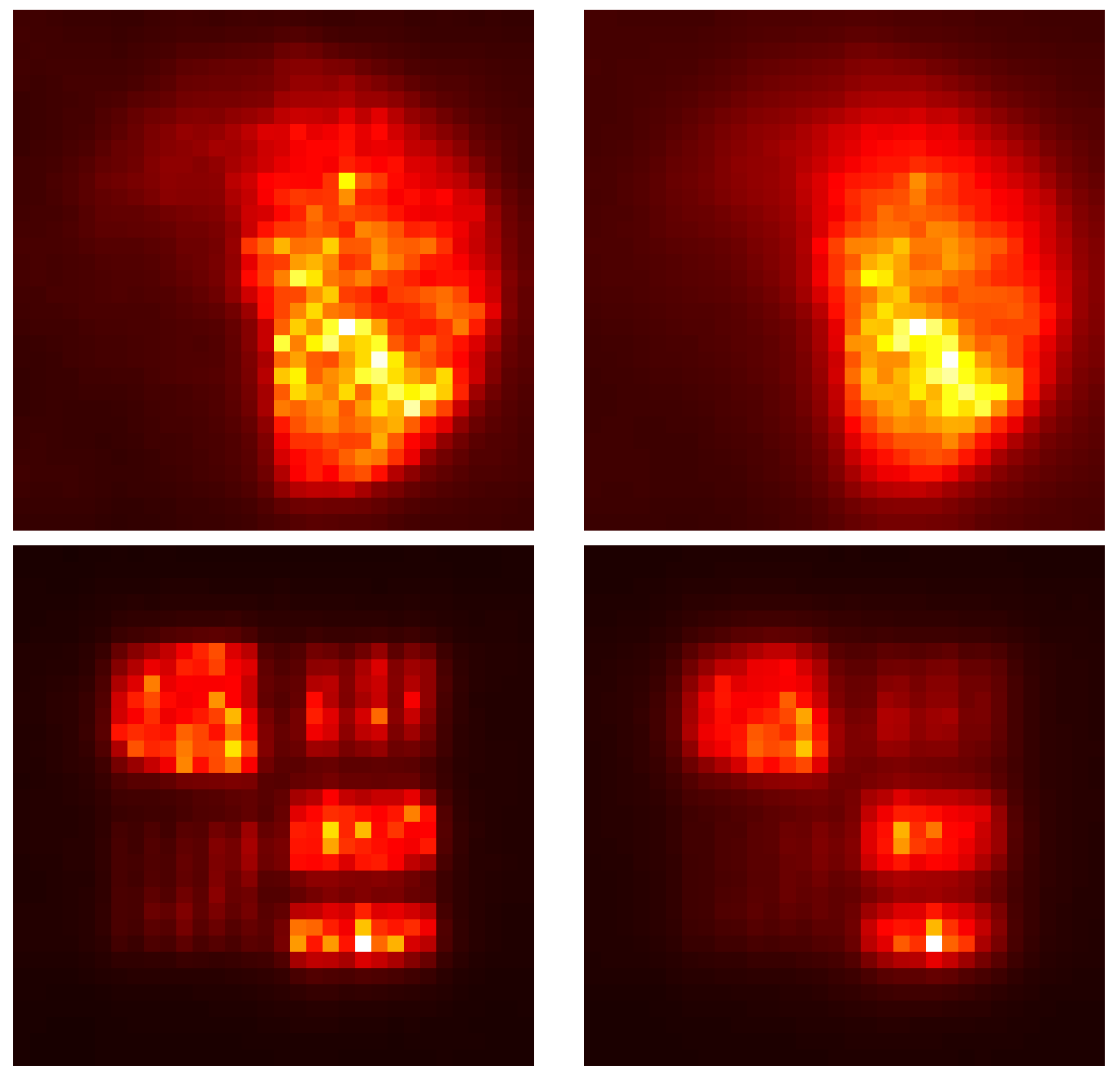
Figure 4 shows the results of 1000 iterations of the EM algorithm using Goods’s roughness penalty for α / ( N M ) = 0.002 and α / ( N M ) = 0.005 .

4.2.3. Silverman’s Roughness

Inspired by the work of Good and Gaskins [59], Silverman [69] suggested alternative penalties that employ differential operators of the logarithm of the function. Like Good’s roughness, Silverman proposed his penalty in the context of density estimation. We consider the special case
x + y ln σ 2 ( x , y ) 2 d x d y .
In the context of optical astronomy, Molina and Ripley [55] suggest smoothing the logarithm of the image, noticing that “astronomers tend to look at the raw data on a logarithmic scale (by choosing contour levels in a geometric progression) except when looking at details at near background level”. Section 5.2.3 in [66] considers the application of (24) to radar imaging.
Discretizing (24) yields
Φ S ( f ) = i 1 , i 2 [ ( ln σ i 1 + 1 , i 2 2 ln σ i 1 , i 2 2 ) 2 + ( ln σ i 1 , i 2 + 1 2 ln σ i 1 , i 2 2 ) 2 ] .
Using this penalty requires solving the following set of nonlinear equations at each iteration of the EM algorithm:
0 = 1 σ i 1 , i 2 2 + σ i 1 , i 2 2 ( u n ) ( Σ ( o l d ) ) ( σ i 1 , i 2 2 ) 2 + α N M 2 σ i 1 , i 2 2 [ ln σ i 1 + 1 , i 2 2 + ln σ i 1 1 , i 2 2 + ln σ i 1 , i 2 + 1 2 + ln σ i 1 , i 2 1 2 4 ln σ i 1 , i 2 2 ] .
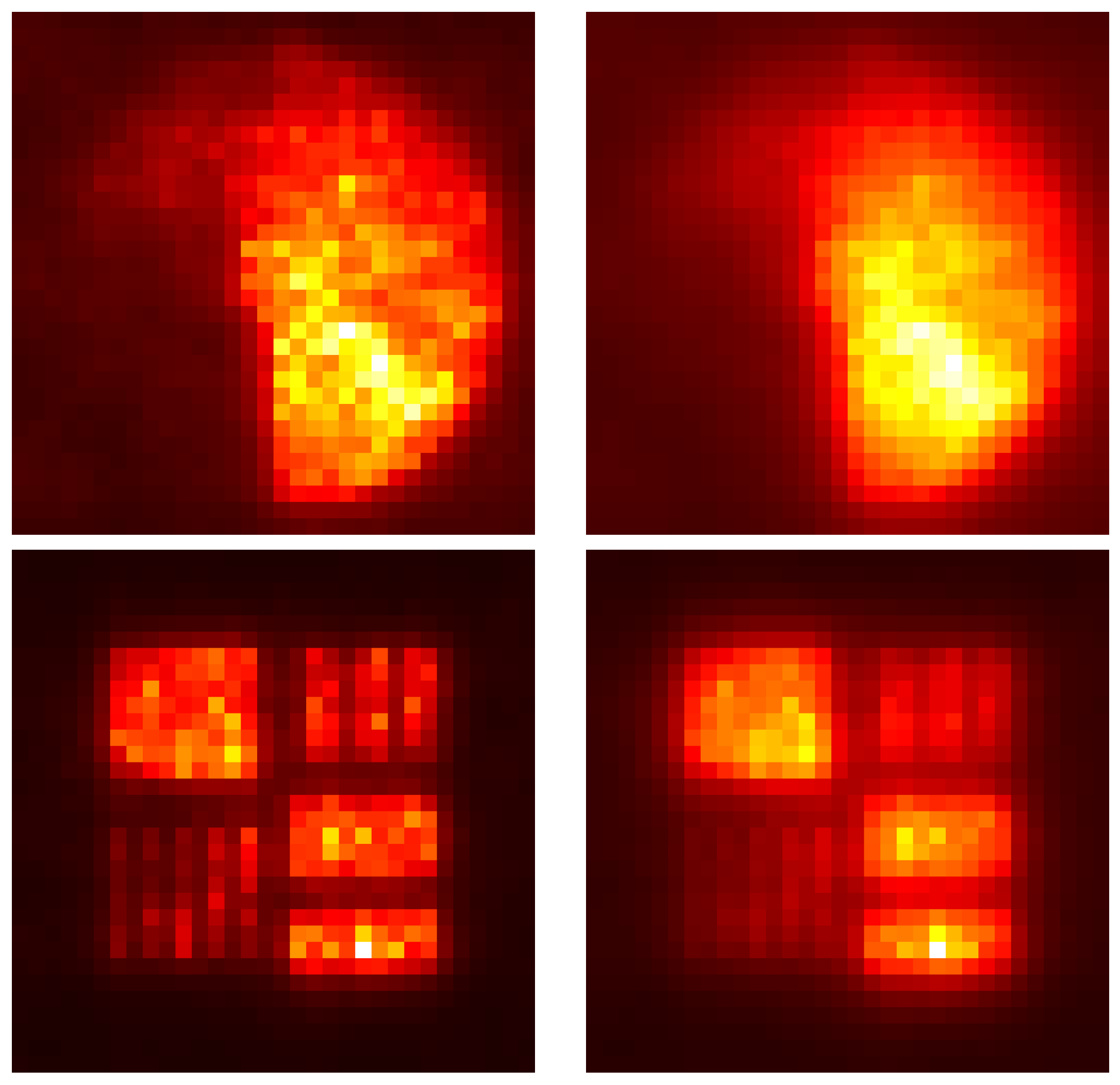
Figure 5 shows the results of 1000 iterations of the EM algorithm using Silverman’s roughness penalty for α / ( N M ) = 0.002 and α / ( N M ) = 0.005 .

4.2.4. General Markov Random Fields

When discretized, Good’s and Silverman’s roughness penalties can be thought of as inducing a prior with a nearest-neighbor Markov random field structure. A wide variety of such priors have been proposed for image reconstruction [70] that could be tried here. For instance, the use of the square in (20) and (24) results in reconstructions that, while less noisy, have smoothed edges. Employing powers less than two results in a penalty that tends to smooth continuous regions while better preserving edges. For simple penalties employing the derivative of the function (instead of the square root or the logarithm as above), this corresponds to a Markov random field with the popular generalized Gaussian distribution [71,72]. Good’s roughness and Silverman’s roughness can be generalized in a similar way. We leave this topic for future work.

4.3. Regularization via General Smoothing Steps

Notice that in the method of penalties, a simple modification of the EM algorithm can be used to produce the penalized likelihood estimates; the resulting algorithm happens to amount to nonlinearly smoothing the result of the maximization step at each iteration before returning to the expectation step. In the fields of emission tomography and stereology, Silverman et al. [73] suggested experimenting with different kinds of smoothing steps. For arbitrary choices of smoothing, the resulting expectation–maximization–smoothing (EMS) algorithm will not, in general, correspond to a particular penalized likelihood method. In addition, it is difficult to determine exactly what such algorithms converge to, if they converge at all. However, considering the success illustrated in [73] for Poisson intensity estimation, we are motivated to explore other kinds of smoothing in our radio astronomy application. One such example is shown in Figure 6, in which the smoothing step is a simple nearest-neighbor linear filter defined by
( L f ) i 1 , i 2 = f i 1 , i 2 + α [ f i 1 + 1 , i 2 + f i 1 1 , i 2 + f i 1 , i 2 + 1 + f i 1 , i 2 1 ] + α 2 [ f i 1 + 1 , i 2 + 1 + f i 1 1 , i 2 + 1 + f i 1 1 , i 2 + 1 + f i 1 1 , i 2 1 ] ,
where α here is a parameter that controls the amount of smoothing.
Applying a linear smoothing step in the EM iteration for emission tomography has a natural relationship to minimizing a penalized likelihood in which the penalty is quadratic in the square root of the intensity (see [74] and Section 5 in [73]), yielding a rather unexpected connection to Good’s roughness of Section 4.2.2. Surprisingly, neither the authors nor the discussants in [73] refer to the work of Good and Gaskins or to its later application in emission tomography. The connection is explicitly noted by Eggermont and LaRiccia [75], however. Latham and Anderssen [76] provided some deep analysis of linear smoothing in the emission tomography iteration. We know of no equivalent existing analysis of adding a linear smoothing step to (10).
Eggermont and LaRiccia [75] proposed smoothing using nonlinear operation N , constructed from a linear smoother L according to N { f } = exp ( L { ln f } ) . When applied to density or Poisson intensity estimation, the resulting EMS algorithm maximizes a particular functional they call a “modified log-likelihood”. This contrasts with other EMS algorithms that do not necessarily correspond to minimizing some particular functional. To our knowledge, there is no parallel body of analysis of EMS algorithms for structured covariance estimation; it remains a wide open area for future work.
For another example, the left column of Figure 7 shows the results of an EMS algorithm that uses a 3 by 3 median filter in the smoothing step. Observe how the EMS algorithm with median smoothing maintains sharp edges and yields a cartoon-like reconstruction; also note that this is not equivalent to median filtering the raw ML estimate of the unconstrained EM algorithm, as shown in the right column of Figure 7.

5. Conclusions

The simulations presented in this paper offer preliminary insight into the behavior of structured covariance estimation techniques for forming radio astronomy images. Without regularization, the resulting estimates (as seen in Figure 3) are unacceptably rough. This is a result of the inherent ill-posed nature of the maximum-likelihood estimation of underlying continuous functions from limited data, and not a fault of the expectation–maximization algorithm itself. The results in Section 4.2.2, Section 4.2.3, and Section 4.3 illustrate that tuning parameters allow for a tradeoff between the noise and blurriness of the reconstruction. More detailed studies should be conducted, including studies with real data, which compare maximum penalized-likelihood estimates and EMS algorithm estimates with the results of traditional procedures such as the CLEAN algorithm and classical maximum-entropy algorithms.
Real radio astronomy measurements exhibit several phenomena that our statistical model currently does not account for. In some radio astronomy arrays, in order to reduce cost, the correlators are “hard-wired” in such a way that only certain correlation measurements are made; thus certain elements of S may be missing. Before correlation, the raw data are often significantly truncated, sometimes as coarsely as one bit, which has an unpleasant effect on the correlation measurement (see Sections 8.3 through 8.5 in [5]). It may be beneficial to explicitly model these effects and derive appropriate extensions to the EM algorithm presented here. There are also a host of calibration issues (particularly in Very Long Baseline Interferometry (VLBI), where the sensor array may span whole continents, [4]) that we have neglected that could also be incorporated into the model and the algorithm. Leshem and van der Veen [13] discuss these calibration issues from a maximum-likelihood viewpoint.
One of the main difficulties with EM algorithms in general is their slow convergence rates. A variety of EM variants have been proposed that boast faster convergence. For instance, the Space-Alternating Generalized EM (SAGE) algorithm of Fessler and Hero [77] updates the parameters in groups instead of all at once; each group has its own associated hidden data space, which would be a complete data space if the remaining parameters were known. Schulz has formulated several SAGE algorithms [78] for maximizing (4) that could be implemented for forming radio astronomy images. The one-dimensional experiments reported in [78] demonstrate the greater likelihood change per iteration of the SAGE algorithm; however, this particular implementation requires around three times the amount of computation per iteration as the original EM implementation. The details of such timing analyses are highly platform-dependent; one could imagine a specialized hardware architecture that could perform the SAGE iterations faster than the EM iterations, or vice versa. In any particular application, one should compare various implementations to find the algorithm with best performance on some given hardware architecture for that particular instance. SAGE algorithms are more convenient for maximizing penalized likelihoods using Markov random field-type penalties, because the SAGE recipe decouples the joint maximization step, which requires solving sets of equations like (23) and (26), into a series of single-parameter maximizations.
As Mhiri et al. pointed out in the right column of p. 3 in [17], their EM algorithm for nonrandom intensity estimation with a compound Gaussian noise model could be extended to other regularization techniques besides the L1-norm they used for point-like images. This could include the Goods/O’Sullivan or Silverman functionals explored in Section 4.2.2 and Section 4.2.3. In the other direction, for inspiration, L1-norm regularization could be used with our algorithm.
An appealing aspect of the statistical formulation is that it allows the prediction of estimator performance via Cramér–Rao bounds. In addition to giving scientists an understanding of the fundamental limits of the available instrumentation, it provides appealing criteria for making design decisions, such as the placement of receiver locations, in various applications. There has been a tremendous amount of work on studying such design choices [79,80] using other kinds of criteria. For large images, inverting the Fisher information can become cumbersome; Hero and Fessler [81] proposed an iterative algorithm for computing Cramér–Rao bounds on parameter subsets that avoids the explicit inversion of the Fisher information matrix via a complete/incomplete data formulation analogous to the EM algorithm.

Funding

This work was supported by a grant from the DARPA (Defense Advanced Research Projects Agency) under Contract F49620-98-1-0498, administered by AFOSR (Air Force Office of Scientific Research).

Data Availability Statement

The MATLAB code and simulated data needed to reproduce the results in this paper are openly available at github.com/lantertronics/radioastem (accessed on 10 December 2024).

Acknowledgments

This paper is dedicated in loving memory of Donald L. Snyder, whose patient guidance over many years inspired this work. We also thank Richard E. Blahut for detailed comments on several drafts of this manuscript.

Conflicts of Interest

The authors declare no conflicts of interest.

Abbreviations

The following abbreviations are used in this manuscript:
EMexpectation–maximization;
SAGEspace-alternating generalized EM;
TLAthree-letter acronym;
LDlinear dichroism.

References

  1. Ryle, M.; Hewish, A. The Synthesis of Large Radio Telescopes. Mon. Not. R. Astron. Soc. 1960, 120, 220–230. [Google Scholar] [CrossRef]
  2. Fomalont, E. Earth-Rotation Aperture Synthesis. Proc. IEEE 1973, 61, 1211–1218. [Google Scholar] [CrossRef]
  3. Goldsmith, P. (Ed.) Instrumentation and Techniques of Radio Astronomy; IEEE Press: New York, NY, USA, 1988. [Google Scholar]
  4. Felli, M.; Spencer, R. (Eds.) Very Long Baseline Interferometry: Techniques and Applications; Kluwer Academic: Dordrecht, The Netherlands, 1989. [Google Scholar]
  5. Thompson, A.; Moran, J.; Swenson, G.W., Jr. (Eds.) Inteferometry and Synthesis in Radio Astronomy, 3rd ed.; Springer: Berlin/Heidelberg, Germany, 2017. [Google Scholar]
  6. Högbom, J. Aperture Synthesis with a Non-Regular Distribution of Interferometer Baselines. Astron. Astrophys. Suppliment Ser. 1974, 15, 417–426. [Google Scholar]
  7. Schwarz, U. Mathematical-Statistical Description of the Iterative Beam Removing Technique (Method CLEAN). Astron. Astrophys. 1978, 65, 345–356. [Google Scholar]
  8. Bose, R.; Freedman, A.; Steinberg, R. Sequence CLEAN: A Modified Deconvolution Technique for Microwave Images of Contiguous Targets. IEEE Trans. Aerosp. Electron. Syst. 2002, 38, 89–97. [Google Scholar] [CrossRef]
  9. Ables, J. Maximum Entropy Spectral Analysis. Astron. Astrophys. Suppliment Ser. 1974, 15, 383–393. [Google Scholar]
  10. Ponsonby, J. An Entropy Measure for Partially Polarized Radiation and its Application to Estimating Radio Sky Polarization Distributions from Incomplete “Aperture Synthesis” Data by the Maximum Entropy Method. Mon. Not. R. Astron. Soc. 1973, 163, 369–380. [Google Scholar] [CrossRef]
  11. Snyder, D.; O’Sullivan, J.; Miller, M. The Use of Maximum-Likelihood Estimation for Forming Images of Diffuse Radar-Targets from Delay-Doppler Data. IEEE Trans. Inf. Theory 1989, 35, 536–548. [Google Scholar] [CrossRef]
  12. Knapp, M.; Robey, F.; Volz, R.; Lind, F.; Fenn, A.; Morris, A.; Silver, M.; Klein, S.; Seager, S. Vector Antenna and Maximum Likelihood Imaging for Radio Astronomy. In Proceedings of the IEEE Aerospace Conference, Big Sky, MT, USA, 5–12 March 2016; pp. 1–17. [Google Scholar]
  13. Leshem, A.; van der Veen, A.J. Radio Astronomical Imaging in the Presence of Strong Radio Interference. IEEE Trans. Inf. Theory 2000, 46, 1730–1747. [Google Scholar] [CrossRef]
  14. Leshem, A.; van der Veen, A.J.; Boonstra, A.J. Multichannel interference mitigation techniques in radio astronomy. IEEE Trans. Inf. Theory 2000, 131, 355–373. [Google Scholar] [CrossRef]
  15. Johnson, D.; Dudgeon, D. Array Signal Processing; Prentice Hall: Englewood Cliffs, NJ, USA, 1993. [Google Scholar]
  16. Grainger, W.; Das, R.; Grainge, K.; Jones, M.; Kneissl, R.; Pooley, G.; Saunders, R. A Maximum-Likelihood Approach to Removing Radio Sources from Observations of the Sunyaev–Zel’dovich effect, with Application to Abell 611. Mon. Not. R. Astron. Soc. 2002, 337, 1207–1214. [Google Scholar] [CrossRef]
  17. Mhiri, Y.; Korso, M.; Breloy, A.; Larzabal, P. Regularized maximum likelihood estimation for radio interferometric imaging in the presence of radiofrequency interferences. Signal Process. 2024, 220, 109430. [Google Scholar] [CrossRef]
  18. Zawadzski, B.; Czekala, I.; Loomis, R.; Quinn, T.; Grzybowski, H.; Frazier, R.; Jennings, J.; Nizam, K.; Jian, Y. Regularized Maximum Likelihood Image Synthesis and Validation for ALMA Continuum Observations of Protoplanetary Disks. Publ. Astron. Soc. Pacific 2023, 135, 064503. [Google Scholar] [CrossRef]
  19. Miller, M.; Fuhrmann, D.R. Maximum likelihood narrow-band direction finding and the EM algorithm. IEEE Acoust. Speech Signal Process. 1990, 38, 560–577. [Google Scholar] [CrossRef]
  20. Kraus, J. Radio Astronomy, 2nd ed.; Cygnus-Quasar Books: Powell, OH, USA, 1986. [Google Scholar]
  21. Burg, J.; Luenberger, D.; Wenger, D. Estimation of Structured Covariance Matrices. Proc. IEEE 1982, 70, 963–974. [Google Scholar] [CrossRef]
  22. Rieken, D.; Fuhrmann, D.; Lanterman, A. Spatial Spectrum Estimation for Time-Varying Arrays using the EM Algorithm. In Proceedings of the 38th Annual Allerton Conference on Communications, Control, and Computing, Monticello, IL, USA, 4–6 October 2000. [Google Scholar]
  23. Fuhrmann, D. Structured Covariance Estimation: Theory, Application, and Recent Results. In Proceedings of the Fourth IEEE Workshop on Sensor Array and Multichannel Processing, Waltham, MA, USA, 12–14 July 2006. [Google Scholar]
  24. Fuhrmann, D. Numerically Stable Implementations of the Structured Covariance Expectation-Maximization Algorithm. SIAM J. Matrix Anal. Appl. 2007, 29, 855–869. [Google Scholar] [CrossRef]
  25. Fuhrmann, D. Structured covariance estimation and radar imaging with sparse linear models. In Proceedings of the 1st IEEE International Workshop on Computational Advances in Multi-Sensor Adaptive Processing, Puerto Vallarta, Mexico, 13–15 December 2005; pp. 8–11. [Google Scholar]
  26. Neyt, X.; Druyts, P.; Acheroy, M.; Verly, J. Structured covariance matrix estimation for the range-dependent problem in STAP. In Proceedings of the Fourth IASTED International Conference on Antennas, Radar and Wave Propagation, Montreal, QC, Canada, 30 May–1 June 2007; pp. 74–79. [Google Scholar]
  27. Hickman, G.; Krolik, J. MIMO field directionality estimation using orientation-diverse linear arrays. In Proceedings of the Conference Record of the 43rd Asilomar Conference on Signals, Systems and Computers, Pacific Grove, CA, USA, 1–4 November 2009. [Google Scholar]
  28. Robey, F. A Covariance Modeling Approach to Adaptive Beamforming and Detection. Ph.D. Dissertation, Department of Electrical Engineering, School of Engineering and Applied Science, Washington University, St. Louis, MO, USA, 1990. [Google Scholar]
  29. Dempster, A.D.; Laird, N.M.; Rubin, D.B. Maximum Likelihood from Incomplete Data via the EM Algorithm. J. R. Stat. Soc. B 1977, 39, 1–38. [Google Scholar] [CrossRef]
  30. Scharf, L. Statistical Signal Processing: Detection, Estimation and Time Series Analysis; Addison-Wesley: Reading, MA, USA, 1991. [Google Scholar]
  31. Poor, V. An Introduction to Signal Detection and Estimation, 2nd ed.; Spinger: New York, NY, USA, 1994. [Google Scholar]
  32. Napier, P.; Thompson, A.; Ekers, R. The Very Large Array: Design and Performance of a Modern Synthesis Radio Telescope. Proc. IEEE 1983, 71, 1295–1320. [Google Scholar] [CrossRef]
  33. Tapia, R.A.; Thompson, J.R. Nonparametric Probability Density Estimation; Johns Hopkins University Press: Baltimore, MD, USA, 1978. [Google Scholar]
  34. Snyder, D.; Miller, M. The Use of Sieves to Stabilize Images Produced with the EM Algorithm for Emission Tomography. IEEE Trans. Nucl. Sci. 1985, 32, 3864–3872. [Google Scholar] [CrossRef]
  35. Snyder, D.; Miller, M.; Thomas, L.J.; Politte, D. Noise and Edge Artifacts in Maximum-Likelihood Reconstruction for Emission Tomography. IEEE Trans. Med. Imaging 1987, 6, 228–237. [Google Scholar] [CrossRef] [PubMed]
  36. Snyder, D.L.; Miller, M.I. Random Point Processes in Time and Space, 2nd ed.; Springer: Berlin/Heidelberg, Germany, 1991. [Google Scholar]
  37. Grenander, U. Abstract Inference; John Wiley and Sons: New York, NY, USA, 1981. [Google Scholar]
  38. Politte, D.; Snyder, D. The Use of Constraints to Eliminate Artifacts in Maximum-Likelihood Image Estimation for Emission Tomography. IEEE Trans. Nucl. Sci. 1988, 35, 608–610. [Google Scholar] [CrossRef]
  39. Politte, D.G.; Snyder, D.L. Corrections for Accidental Coincidences and Attenuation in Maximum-Likelihood Image Reconstruction for Positron-Emission Tomography. IEEE Trans. Med. Imaging 1991, 10, 82–89. [Google Scholar] [CrossRef]
  40. Moulin, P.; O’Sullivan, J.; Snyder, D. A Method of Sieves for Multiresolution Spectrum Estimation and Radar Imaging. IEEE Trans. Inf. Theory 1992, 38, 801–813. [Google Scholar] [CrossRef]
  41. O’Sullivan, J.; Snyder, D.; Porter, D.; Moulin, P. An Application of Splines to Maximum Likelihood Radar Imaging. Int. J. Imaging Syst. Technol. 1992, 4, 256–264. [Google Scholar] [CrossRef]
  42. Moulin, P. A Wavelet Regularization Method for Diffuse Radar-Target and Speckle-Noise Reduction. J. Math. Imaging Vis. 1993, 3, 123–134. [Google Scholar] [CrossRef]
  43. Frieden, B.R. Restoring with maximum likelihood and maximum entropy. J. Opt. Soc. Am. 1972, 62, 511–518. [Google Scholar] [CrossRef] [PubMed]
  44. Erickson, G.; Smith, C. (Eds.) Maximum-Entropy and Bayesian Methods in Science and Engineering; Kluwer Academic: Dordrecht, The Netherlands, 1988. [Google Scholar]
  45. Amato, U.; Hughes, W. Maximum entropy regularization of Fredholm integral equations of the first kind. Inverse Probl. 1991, 7, 793–808. [Google Scholar] [CrossRef]
  46. Mead, L. Approximate solution of Fredholm integral equations by the maximum entropy method. J. Math. Phys. 1986, 27, 2903–2907. [Google Scholar] [CrossRef]
  47. Skilling, J.; Strong, A.W.; Bennett, K. Maximum-entropy image processing in gamma-ray astronomy. Mon. Not. R. Astr. Soc. 1979, 187, 145–152. [Google Scholar] [CrossRef]
  48. Skilling, J.; Bryan, R. Maximum entropy image reconstruction: General algorithm. Mon. Not. R. Astron. Soc. 1984, 211, 111–124. [Google Scholar] [CrossRef]
  49. Frieden, B.; Wells, D.C. Restoring with maximum entropy. III. Poisson sources and backgrounds. J. Opt. Soc. Am. 1978, 68, 93–103. [Google Scholar] [CrossRef]
  50. Gull, S.; Daniell, G. The maximum entropy algorithm applied to image enhancement. Proc. IEEE 1980, 5, 170. [Google Scholar]
  51. Wernecke, S.; D’Addario, L. Maximum entropy image reconstruction. IEEE Trans. Comput. 1977, 26, 351–364. [Google Scholar] [CrossRef]
  52. Narayan, R.; Nityananda, R. Maximum Entropy Image Restoration in Astronomy. Annu. Rev. Astron. Astrophys. 1986, 24, 127–170. [Google Scholar] [CrossRef]
  53. Shioya, H.; Gohara, K. Maximum Entropy Method for Diffractive Imaging. J. Opt. Soc. Am. A 2008, 25, 2846–2850. [Google Scholar] [CrossRef] [PubMed]
  54. Moran, P. Observations on Maximum Entropy Processing of MR Images. Magn. Reson. Imaging 1991, 9, 213–221. [Google Scholar] [CrossRef]
  55. Molina, R.; Ripley, B. Using Spatial Models as Priors in Astronomical Image Analysis. J. Appl. Stat. 1989, 16, 193–206. [Google Scholar] [CrossRef]
  56. Donoho, D.; Johnstone, I.; Hoch, J.; Stern, A. Maximum Entropy and the Nearly Black Object. J. R. Stat. Soc. B 1992, 54, 41–81. [Google Scholar] [CrossRef]
  57. Narayan, R.; Nityananda, R. Maximum Entropy—Flexibility Versus Fundamentalism. In Indirect Imaging; Roberts, J., Ed.; Cambridge University Press: Cambridge, UK, 1984; pp. 281–290. [Google Scholar]
  58. Gupta, A.; Nagar, D. Matrix Variate Distributions; Chapman and Hall/CRC: Boca Raton, FL, USA, 1999. [Google Scholar]
  59. Good, I.J.; Gaskins, R.A. Nonparametric roughness penalties for probability densities. Biometrika 1971, 58, 255–277. [Google Scholar] [CrossRef]
  60. Miller, M.; Roysam, B. Bayesian Image Reconstruction for Emission Tomography Incorporating Good’s Roughness Prior on Massively Parallel Processors. Proc. Natl. Acad. Sci. USA 1991, 88, 3223–3227. [Google Scholar] [CrossRef] [PubMed]
  61. McCarthy, A.; Miller, M. Maximum Likelihood SPECT in Clinical Computation Times Using Mesh-Connected Parallel Computers. IEEE Trans. Med. Imaging 1991, 10, 426–436. [Google Scholar] [CrossRef]
  62. Butler, C.; Miller, M. Maximum A Posteriori Estimation for SPECT Using Regularization Techniques on Massively-Parallel Computers. IEEE Trans. Med. Imaging 1993, 12, 84–89. [Google Scholar] [CrossRef] [PubMed]
  63. Miller, M.; Butler, C. 3-D Maximum A Posteriori Estimation for SPECT on Massively-Parallel Computers. IEEE Trans. Med. Imaging 1993, 12, 560–565. [Google Scholar] [CrossRef] [PubMed]
  64. Butler, C.S.; Miller, M.; Miller, T.R.; Wallis, J.W. Massivel parallel computers for 3D single-photon-emission computed tomography. Phys. Med. Biol. 1994, 39, 575–582. [Google Scholar] [CrossRef] [PubMed]
  65. Joshi, S.; Miller, M. Maximum a posteriori Estimation with Good’s Roughness for Optical Sectioning Microscopy. Opt. Soc. Am. A 1993, 10, 1078–1085. [Google Scholar] [CrossRef] [PubMed]
  66. Lanterman, A. Statistical Radar Imaging of Diffuse and Specular Targets Using an Expectation-Maximization Algorithm. In Proceedings of the Algorithms for Synthetic Aperture Radar Imagery VII, Orlando, FL, USA, 24–28 April 2000; Volume SPIE Proc. 4053, pp. 20–31. [Google Scholar]
  67. O’Sullivan, J. Roughness Penalties on Finite Domains. IEEE Trans. Image Process. 1995, 4, 1258–1268. [Google Scholar] [CrossRef]
  68. Frieden, B. Some Analytical and Statistical Properties of Fisher Information. In Proceedings of the Stochastic and Neural Methods in Signal Processing, Image Processing, and Computer Vision, San Diego, CA, USA, 24–26 July 1991; Volume SPIE Proc. 1569. [Google Scholar]
  69. Silverman, B.W. On the Estimation of a Probability Density Function by the Maximum Penalized Likelihood Method. Ann. Stat. 1982, 10, 795–810. [Google Scholar] [CrossRef]
  70. Geman, D.; Reynolds, G. Constrained Restoration and the Recovery of Discontinuities. IEEE Trans. Pattern Anal. Mach. Intell. 1992, 14, 367–383. [Google Scholar] [CrossRef]
  71. Bouman, C.; Sauer, K. A Generalized Gaussian Image Model for Edge-Preserving MAP Estimation. IEEE Trans. Image Process. 1993, 2, 296–310. [Google Scholar] [CrossRef] [PubMed]
  72. Chen, J.; Nunez-Yanez, J.; Achim, A. Video Super-resolution Using Generalized Gaussian Markov Random Fields. IEEE Signal Process. Lett. 2012, 19, 63–66. [Google Scholar] [CrossRef]
  73. Silverman, B.; Jones, M.; Wilson, J.; Nychka, D. A Smoothed EM Approach to Indirect Estimation Problems, with Particular Reference to Stereology and Emission Tomography (with discussion). J. R. Stat. Soc. B 1990, 52, 271–324. [Google Scholar] [CrossRef]
  74. Nychka, D. Some Properties of Adding a Smoothing Step to the EM Algorithm. Stat. Probab. Lett. 1990, 9, 187–193. [Google Scholar] [CrossRef]
  75. Eggermont, P.; LaRiccia, V. Maximum Smoothed Likelihood Density Estimation for Inverse Problems. Ann. Stat. 1995, 23, 199–220. [Google Scholar] [CrossRef]
  76. Latham, G.; Anderssen, R. On the Stabilization Inherent in the EMS Algorithm. Inverse Probl. 1994, 10, 793–808. [Google Scholar] [CrossRef]
  77. Fessler, J.; Hero, A. Space-Alternating Generalized Expectation-Maximization Algorithm. IEEE Trans. Signal Process. 1994, 42, 2664–2677. [Google Scholar] [CrossRef]
  78. Schulz, T. Penalized Maximum-Likelihood Estimation of Covariance Matrices with Linear Structure. IEEE Trans. Signal Process. 1997, 45, 3027–3038. [Google Scholar] [CrossRef]
  79. Chow, Y. On Designing a Supersynthesis Antenna Array. IEEE Trans. Antennas Propag. 1972, 20, 30–35. [Google Scholar] [CrossRef]
  80. Mathur, N. A Pseudodynamic Programming Technique for the Design of a Correlator Supersynthesis Array. Radio Sci. 1969, 4, 235–243. [Google Scholar] [CrossRef]
  81. Hero, A.; Fessler, J. A Recursive Algorithm for Computing Cramer-Rao-Type Bounds on Estimator Covariance. IEEE Trans. Inf. Theory 1994, 40, 1205–1210. [Google Scholar] [CrossRef]
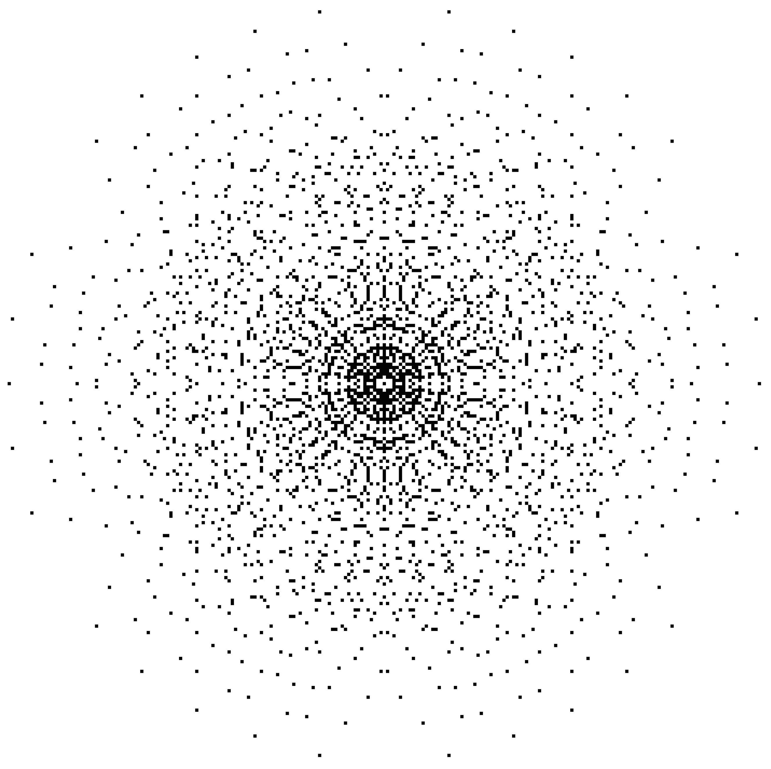
Figure 1. Fourier sampling pattern associated with the simulated scenario.
Stats 07 00088 g001
Figure 2. Top row: two 32 × 32 ideal intensity functions used in the simulations. Bottom row: traditional “dirty maps” formed from simulated data. Images in this paper are displayed using MATLAB’s “hot” colormap.
Stats 07 00088 g002
Figure 3. Results of the unconstrained EM algorithm for two different data sets (shown in different rows). From left to right, the columns show results at 100, 200, and 1000 iterations.
Stats 07 00088 g003aStats 07 00088 g003b
Figure 4. Results of 1000 iterations of the EM algorithm using Good’s roughness penalty with α / ( N M ) = 0.002 (left column) and α / ( N M ) = 0.005 (right column).
Stats 07 00088 g004
Figure 5. Results of 1000 iterations of the EM algorithm using Silverman’s roughness penalty with α / ( N M ) = 0.002 (left column) and α / ( N M ) = 0.005 (right column).
Stats 07 00088 g005
Figure 6. Results of 1000 iterations of an EMS algorithm using the linear smoothing step defined by (27) for α = 0.001 (left column) and α = 0.003 (right column).
Stats 07 00088 g006
Figure 7. The left column shows the results of 1000 iterations of the EMS algorithm using a nearest-neighbor median filter as the smoothing step. The right column shows the results of median filtering 1000 iterations with the unconstrained EM algorithm.
Stats 07 00088 g007aStats 07 00088 g007b
Disclaimer/Publisher’s Note: The statements, opinions and data contained in all publications are solely those of the individual author(s) and contributor(s) and not of MDPI and/or the editor(s). MDPI and/or the editor(s) disclaim responsibility for any injury to people or property resulting from any ideas, methods, instructions or products referred to in the content.