Article

Direct and Indirect Effects of Environmental and Socio-Economic Factors on COVID-19 in Africa Using Structural Equation Modeling

by
Bissilimou Rachidatou Orounla
1,*,†,
Ayédèguè Eustache Alaye
1,†,
Kolawolé Valère Salako
1,
Codjo Emile Agbangba
1,2,
Justice Moses K. Aheto
3 and
Romain Glèlè Kakaï
1
1
Laboratory of Biomathematics and Forest Estimation, Faculty of Agronomic Sciences, University of Abomey-Calavi, Cotonou 04 BP 1525, Benin
2
Ecole Polytechnique d’Abomey-Calavi, Université d’Abomey-Calavi, Cotonou 04 BP 1525, Benin
3
Department of Biostatistics, School of Public Health, College of Health Sciences, University of Ghana, Legon-Accra P.O. Box LG13, Ghana
*
Author to whom correspondence should be addressed.
These authors contributed equally to this work.
Stats 2024, 7(3), 1051-1065; https://doi.org/10.3390/stats7030062
Submission received: 13 August 2024 / Revised: 10 September 2024 / Accepted: 13 September 2024 / Published: 19 September 2024

Abstract

:
Understanding direct and indirect relationships of environmental, socio-economic and climate variables and the dynamics of epidemics is key to guiding targeted public health policy and interventions. This study investigates the direct and indirect effects of environmental and socio-economic factors on the COVID-19 dynamics in Africa (54 African countries from 2019 to 2021) using SEM approach. Specifically, the study aimed to: (i) assess the performance of two SEM estimation methods (Lisrel and PLS-SEM) in relationship to sample size (100, 200, 500, and 1000) and level of model complexity (No, two, and four indirect effects) and (ii) use the most performing SEM estimation method to examine direct and indirect effects of factors influencing the number of cases and deaths of COVID-19 in Africa. The results highlight a positive spatial correlation between factors such as temperature, humidity, age, the proportion of people aged over 65, and the COVID-19 incidence. Under the control of confounding factors, Lisrel turns out to be the most performing method, identifying climate, demographic and economic factors as the main determinants of COVID-19 dynamics. These factors have a direct and significant impact on the incidence of COVID-19. An indirect relationship was also observed between economic factors and the incidence of COVID-19 through air pollutants. The results highlight the importance of considering these factors in understanding the spread of the virus to avoid further disasters.

1. Introduction

In 2019, the world experienced the emergence of the SARS-CoV-2 virus responsible for the COVID-19 disease in Wuhan, characterized by its rapid spread and high mortality [1,2]. The COVID-19 pandemic caused more than 600 million cases and 6 million deaths globally [3], sparking global interest in understanding disparities in the distribution of cases and deaths [4,5]. Global research has explored risk factors, highlighting the importance of understanding vulnerable groups for targeted interventions [4]. Indeed, geographic heterogeneity has led to questions about the links between the spread of the virus and environmental, climatic, and socio-economic factors, notably temperature and humidity [6,7,8]. The influence of environmental and socio-economic factors on the dynamics of COVID-19 has been well demonstrated at several levels. It has also been reported that some of these parameters and infections exhibit spatial and temporal autocorrelation [9]. Thus, individually assessing the relationship between these parameters and the dynamics of the virus could introduce biases into the estimates, particularly due to spatio-temporal autocorrelations [9]. In this context, simultaneous consideration of environmental and socio-economic factors could make it possible to reduce this bias and better assess their influence on the dynamics of COVID-19. The Structural Equation Modeling (SEM) method has proved to be the most appropriate for simultaneously modeling and estimating with more precision the complex relationships between several dependent and independent variables [10]. This method is an extension of traditional linear modeling techniques, combining factor analysis and linear regression (multiple regression analysis or analysis of variance). SEM aims to understand the relationship between latent constructs (factors), usually indicated by different measures [11]. Two estimation methods predominate in practice for assessing the links between variables in SEM namely Lisrel method and Partial Least Squares SEM (PLS-SEM) [10]. Lisrel method is based on a covariance matrix and PLS-SEM is based on a variance matrix (partial least squares). Usually, CB-SEM requires that the data be normal, while PLS-SEM is quite lenient in this regard [11]. Nevertheless, it is crucial to note that despite emerging debates about the two SEM methods, few studies have truly gone into depth to compare their performance. The rare existing studies have often been limited to summary comparisons (sample size and data distribution) and have been carried out in contexts different from that of epidemiology [11]. Both the sample size and the level of model complexity could have a significant impact on the performance of each of the Lisrel method and Partial Least Squares SEM method, and the precision of the resultant estimates especially in the field of epidemiology. The present study therefore aimed to (i) assess the performance of the two methods in relationship to sample size and level of model complexity and (ii) use the most performing method to explore direct and indirect factors influencing the number of cases and deaths of COVID-19 in Africa.

2. Materials and Methods

2.1. Study Area

No African country has been spared by this pandemic, requiring every nation on the continent to be considered. A spatial analysis of the distribution of incidence and mortality rates of COVID-19 performed by [12] shows significant spatial variability in the intensity of this pandemic across the continent. For example, the authors found 3 regions with a higher incidence of COVID-19 including Egypt and Libya in the northeast, Morocco, Mauritania, Senegal and Gambia in the northwest and Namibia in the south. Similarly, 2 regions with a higher COVID-19 mortality rate were identified, namely in the north-east and north-west parts of the continent, which correspond to regions with high COVID-19 incidence rates. These results illustrate the heterogeneity of the intensity of COVID-19 across the continent and the need to study the factors determining this variability. To provide a comprehensive overview of the impact of the pandemic in Africa, taking into account a variety of environmental and socio-economic contexts, all 54 African countries were therefore considered.

2.2. Data Collection

From the literature review carried out, several variables have been identified as the main determinants of the dynamics of COVID-19, including temperature, humidity, concentrations of carbon dioxide ( ( C O 2 ) ), ozone ( ( O 3 ) ), sulfur dioxide ( S O 2 ) , nitrogen dioxide ( N O 2 ) , particles with a diameter of less than 10 micrometers ( P M 10 ) and those with a diameter of less than 2.5 micrometers( P M 2.5 ). However, due to the unavailability of specific environmental data, particularly those related to pollutants ( P M 2.5 ; ( P M 10 ) ; ( O 3 ) and ( S O 2 ) ), this study focused on four main environmental variables: temperature, relative humidity, ( C O 2 ) and ( N O 2 ) . In addition to environmental parameters, this study also collected socio-economic data known for their potential impact on the dynamics of COVID-19. These data include population density, the median age of the population at the level of each country, expenditure related to imports and exports, the national Gross Domestic Product (GDP) from the industrial sector and then the total expenditure from the tourism sector.
Apart from the above variables, the study took into account confounding factors related to the management of the COVID-19 pandemic. These factors include, in particular, the overall government response index, the containment and health index, and the vaccination policy characterized by the availability of vaccines in each country. These indicators of government response are taken from the Oxford COVID-19 Government Response Tracker (OxCGRT), which provides a range of government responses to the COVID-19 crisis. The purpose of including these indices is to control for them in the final model to better assess the individual effect of the factors considered in this study. The response variables were the incidence of COVID-19, in particular the number of cases and deaths. All these variables were collected at the level of each of the 54 African countries and cover the period 2019 to 2021. Table 1 summarizes the various variables, detailing the sources from which these data were extracted, the effects of each variable, as well as previous studies supporting the expected effects on the evolution of the pandemic.

2.3. Statistical Analyses

2.3.1. Assessing the Spatial Patterns of Environmental, Socio-Economic Variables and Cases of COVID-19

A spatial analysis was carried out using QGis software [19]. The annual mean values of various environmental, social and economic variables, as well as COVID-19 cases and associated deaths, were mapped spatially. The Moran index [20] was used to assess the spatial dependence of each covariate. If the weight of the neighbor pairs ( m = i = 1 n j = 1 n w i j ) is equal to the number of individuals i, then m is equal to n. So, the Moran index can be written as follows:
I Moran = i = 1 n j = 1 n w i j x i x ¯ x j x ¯ i n x i x ¯ 2
where, w i j are the elements of the matrix of spatial interactions, defined in the form of contiguity, distances or national borders; where each spatial unit (country) was associated with a binary value. n is the total number of individuals in the sample.
The Moran index compares the covariance between spatially adjacent observations to the total sample variance, with values ranging from −1 to 1, indicating perfect dispersion to perfect correlation. A contiguity matrix was constructed to determine the spatial proximity between units (countries) based on common borders. Results were interpreted using the Moran plot, which represents the spatial correlation of variables, with a positive or negative slope indicating positive or negative spatial autocorrelation, respectively. This analysis helped to understand the spatial patterns in environmental, social and economic variables, as well as the impact of COVID-19.

2.3.2. Comparing the Performance of the Lisrel and Partial Least Square Estimation Methods Used in the Case of SEM Models

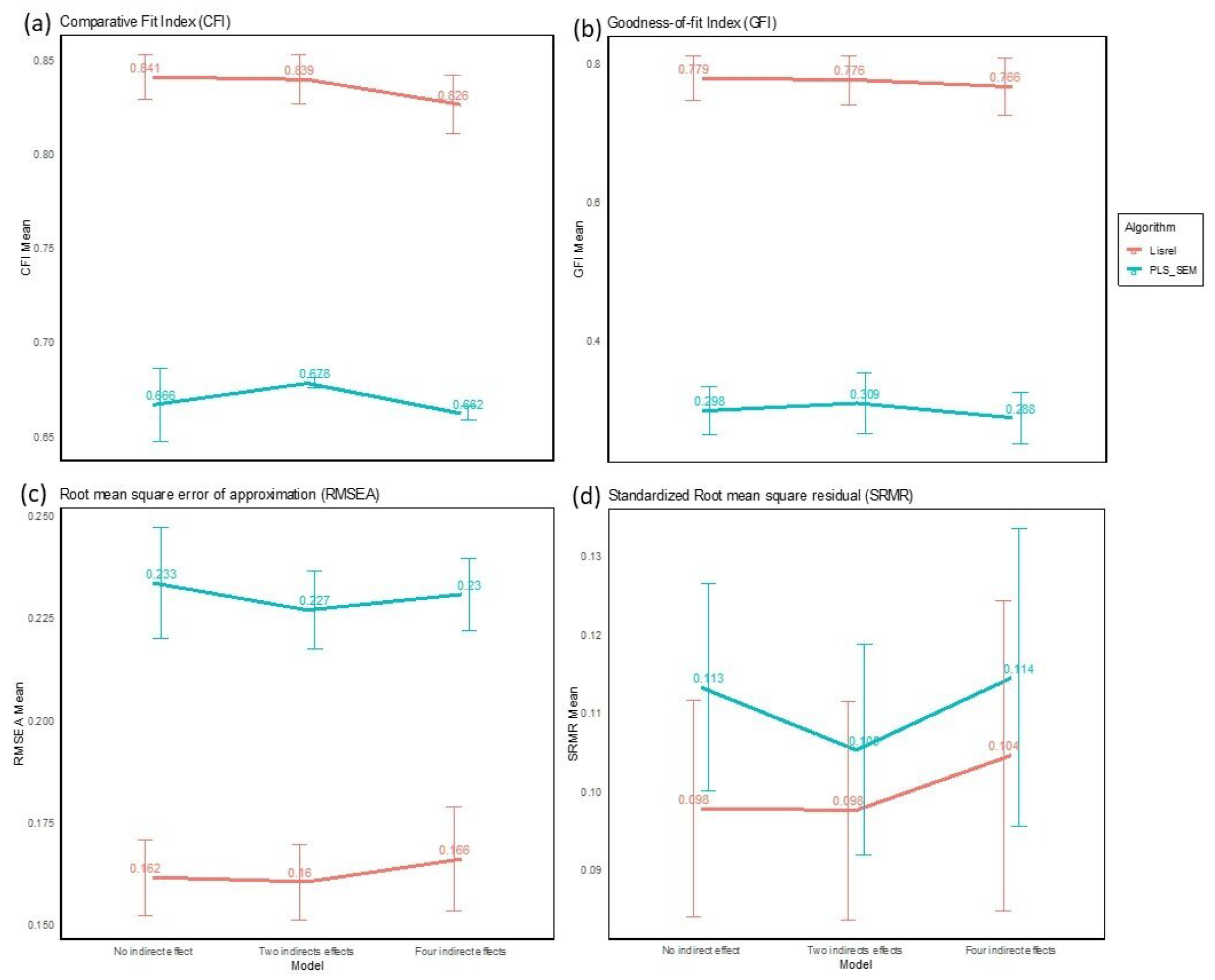
The evaluation of performance of the two estimation methods was assessed in relationship to sample size and the complexity of the model. For the sample size, resampling was performed to generate four sample sizes (n = 100; n = 200; n = 500 and n = 1000) from the original data using bootstrap with replacement for SEM. The model complexity was related to the number of indirect effects: a model with no indirect effects, a model with two indirect effects, and a model with four indirect effects. Figure 1 summarizes the overall methodology used to compare the two estimation methods. The performance of the two estimation methods was evaluated using indices such as Comparative Fit Index (CFI), Goodness-of-fit Index (GFI), Root mean square error of approximation (RMSEA) and Standardized Root mean square residual (SRMR) which were calculated for each sample and each trained model. An RMSEA or SRMR value between 0 and 0.05 indicates an excellent fit; between 0.05 and 0.08 it’s an acceptable approximation error [11]. A CFI value between 0.97 and 1 indicates a good fit, but it’s acceptable between 0.95 and 0.97. The value indicating an excellent fit of GFI is between 0.95 and 1, but 0.90 and 0.95 means an acceptable fit. The mean values of these indices were plotted against sample size and model complexity which helped to identify the best-performing method. Pairwise multiple comparisons with the Bonferroni method of adjusting p-values using the agricolae R package were further performed to test the significance of the observed differences between both methods.

2.3.3. Assessing the Direct and Indirect Effects of Environmental and Socio-Economic Variables on the Incidence of COVID-19 Using the Most Performing Estimation Method

To evaluate the real effects (direct and indirect) of the different variables on COVID-19, the study used the most effective estimation method to model the relationship between the studied variables, while including confounding factors to control their effects. The model coefficients were estimated using the estimation method identified as the most efficient.
The analysis was performed using Rstudio software with SEMinR, cSEM, semPlot, lavaan, dplyr and agricolae packages.

3. Results

3.1. Spatial Patterns of Environmental, Socio-Economic Factors and Incidence of COVID-19

3.1.1. Spatial Analysis

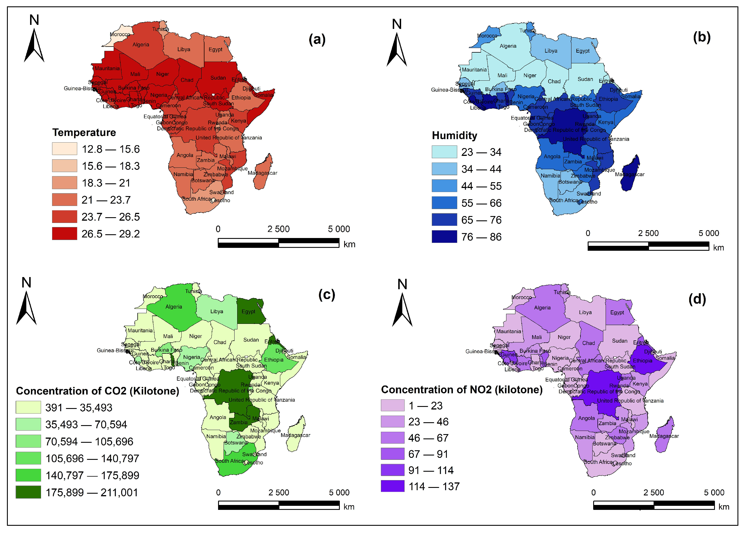
Figure 2 shows the spatial patterns of average values of climate (temperature and humidity) and environmental ( C O 2 and N O 2 emissions) variables from 2019 to 2021. Considerable regional disparities are observed within each country for all variables (Figure 2a–d). Indeed, regional variability highlights higher temperatures in the western zone and higher humidity in the central zone (Figure 2a,b). Concerning climate parameters, significant disparities emerge when comparing regions. Particularly, West Africa stands out with the highest temperatures, ranging between 26.5 °C and 29.2 °C on average, while the southern zone, particularly Lesotho (less than 16 °C on average) and South Africa (less than 19 °C on average), records the lowest temperatures (Figure 2a). On the other hand, relative humidity shows strong fluctuations among countries. Indeed, countries of the central Africa (e.g., Equatorial Guinea, Rwanda, DRC Congo) and some countries of the west Africa (e.g., Sierra Leone, Liberia, Guinea, and Togo) stand out as the regions with the highest humidity rate (76–87%). In the eastern part, there are countries like Madagascar with the same level of humidity (76–87%). On the other hand, the driest areas were mainly found in the western Africa (e.g., Mauritania, Mali, Niger, Burkina Faso) and some in the center (Chad) and the north (Sudan) with an average humidity of between 23–34%. These variations can influence the transmission of COVID-19. C O 2 and N O 2 emissions (Figure 2c,d) show significant differences among regions, indicating varying levels from one area to another with higher levels in the northern, central and southern zones of the continent. Indeed, some countries scattered in the different zones of Africa, notably Eritrea (East zone), Togo (West zone), Egypt (North zone), DRC (central zone), and Zambia (southern zone), present high levels of C O 2 emissions, exceeding 159,000 kilotons, while the majority of countries in the Western zone display significantly lower levels (less than 50,000 kilotons). It is noteworthy that most of the countries with high C O 2 concentrations also have high N O 2 emissions, such as Egypt, Algeria, DRC, Ethiopia, Eritrea, etc. (Figure 2c,d). This regional variability in climatic and environmental parameters could have direct and indirect implications on the dynamics of the pandemic.
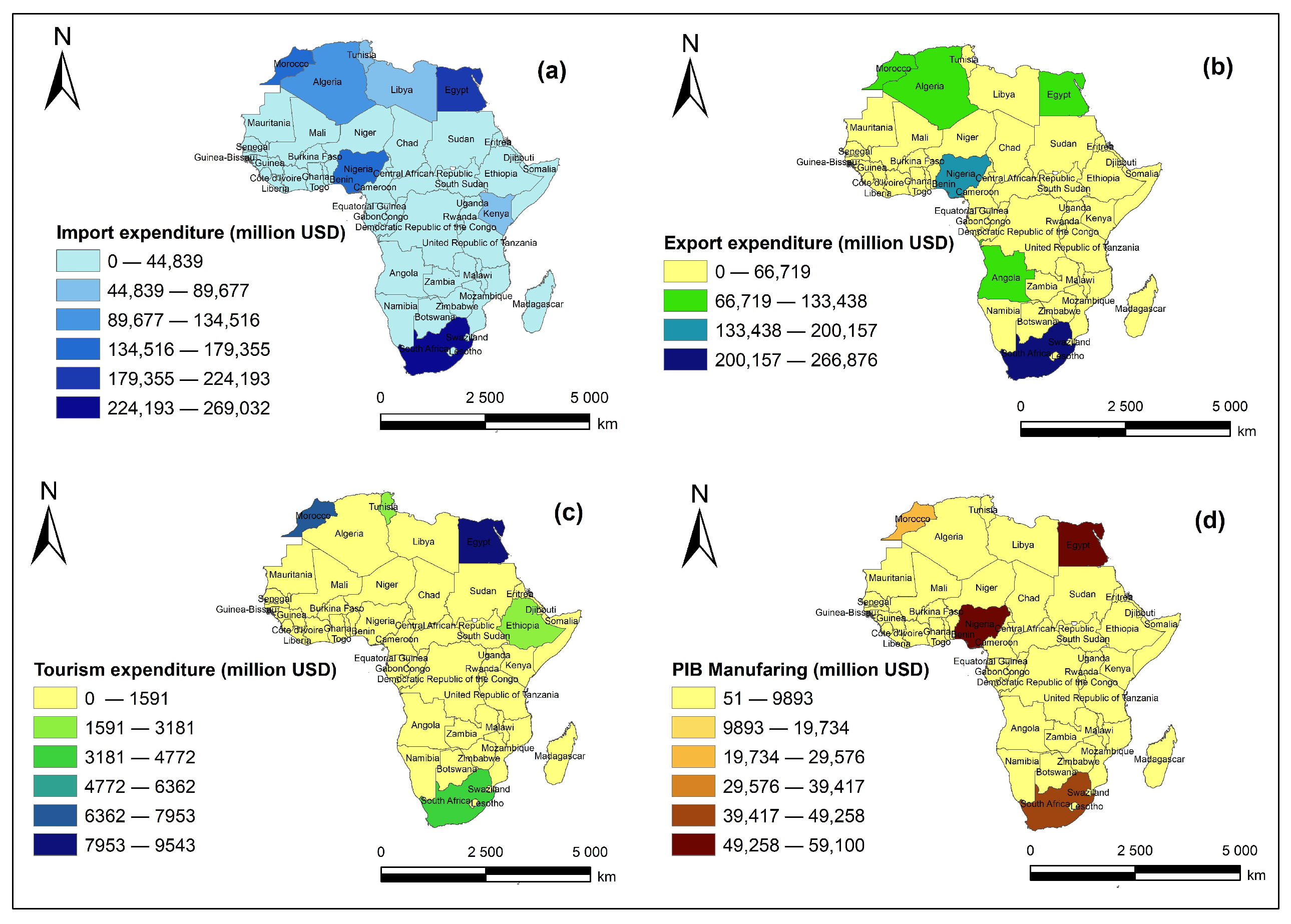
The spatial models of economic factors over three years (2019–2021) match the findings made on environmental and climatic parameters (Figure 3). Indeed, the spatial analysis reveals significant spatial variations in expenditure related to imports and exports (Figure 3a,b). In particular, it highlights that the countries of North Africa, such as Algeria, Egypt, Morocco and Tunisia and those of the South (especially South Africa), display substantial economic expenditure compared to other regions. Concerning tourism expenditure and the GDP of the industrial sector, projections confirm that countries in the North and South (South Africa) maintain considerable levels, averaging over 9 billion (Figure 3c,d). This could increase the risk of introduction and the spread of the virus through tourism.
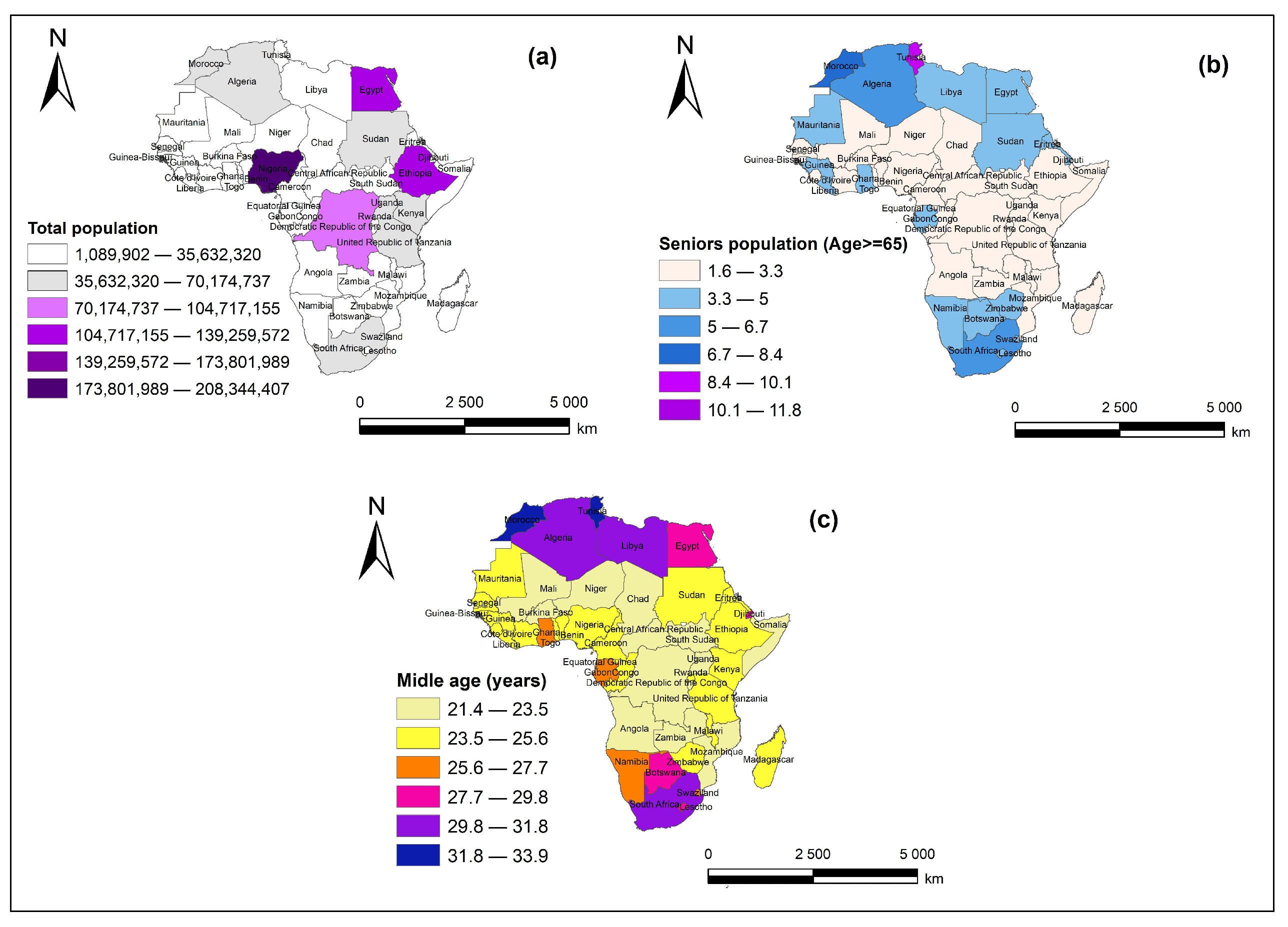
Figure 4 shows the spatial analysis of the average total population and proportion of senior people by country. The analysis of average populations across African countries highlights significant variations, with Nigeria emerging as the most populous nation followed by densely populated countries like those in the eastern, central, and northern regions. Conversely, smaller countries such as Seychelles, Mauritius, and Cape Verde exhibit high population densities due to their compact size (Figure 4a). Notably, North African countries like Tunisia, Morocco, and Libya have substantial proportions of elderly populations (Figure 4b), suggesting higher vulnerability to COVID-19. Conversely, countries like Uganda and Zambia have lower proportions of elderly individuals, impacting pandemic dynamics differently. This demographic diversity underscores the need for tailored prevention and response strategies considering each country’s unique demographic structure and susceptibility to COVID-19.
The spatial patterns of the average incidence of cases and deaths due to COVID-19 (total number of cases and total number of deaths per 10,000 inhabitants) across African countries also shows some differences in the intensity of this pandemic across the continent (Figure 5). Indeed, by examining the map showing the cumulative number of cases per 10,000 inhabitants per country, we see a small variation between the different zones (Figure 5a). Thus, only South Africa stands out from other regions of the continent with a total number of cases greater than 3 million for around 90,000 deaths in total. Furthermore, the countries of the northern zone also stand out slightly from other countries, particularly compared to the western part of the continent. These disparities, even slight, can be linked to the different variables (environmental, economic and demographic) as described above.

3.1.2. Spatial Autocorrelation Testing

The Moran index reveals significant trends. Temperature and relative humidity exhibit a strong spatial positive correlation, indicating that geographically close regions, particularly neighboring countries, tend to share similar values for these environmental parameters (Table 2). In contrast, carbon dioxide ( C O 2 ) and nitrogen dioxide ( N O 2 ) emissions do not show significant spatial dependence, suggesting a relatively random distribution. Economic indicators such as import expenditure, exports, tourism expenditure and manufacturing GDP do not show significant spatial positive correlation, suggesting unpredictable spatial patterns for these activities. Furthermore, population density and demographic variables, such as average age and the proportion of elderly people, show a significant spatial positive correlation although relatively weak. Finally, the incidence of the pandemic, such as the number of cases and deaths per 10,000 inhabitants, exhibits positive spatial dependence, indicating that geographically close regions tend to experience similar impacts.

3.2. Performance of the Lisrel and Partial Least Square Estimation Methods in SEM Models

3.2.1. Comparison Based on Sample Size

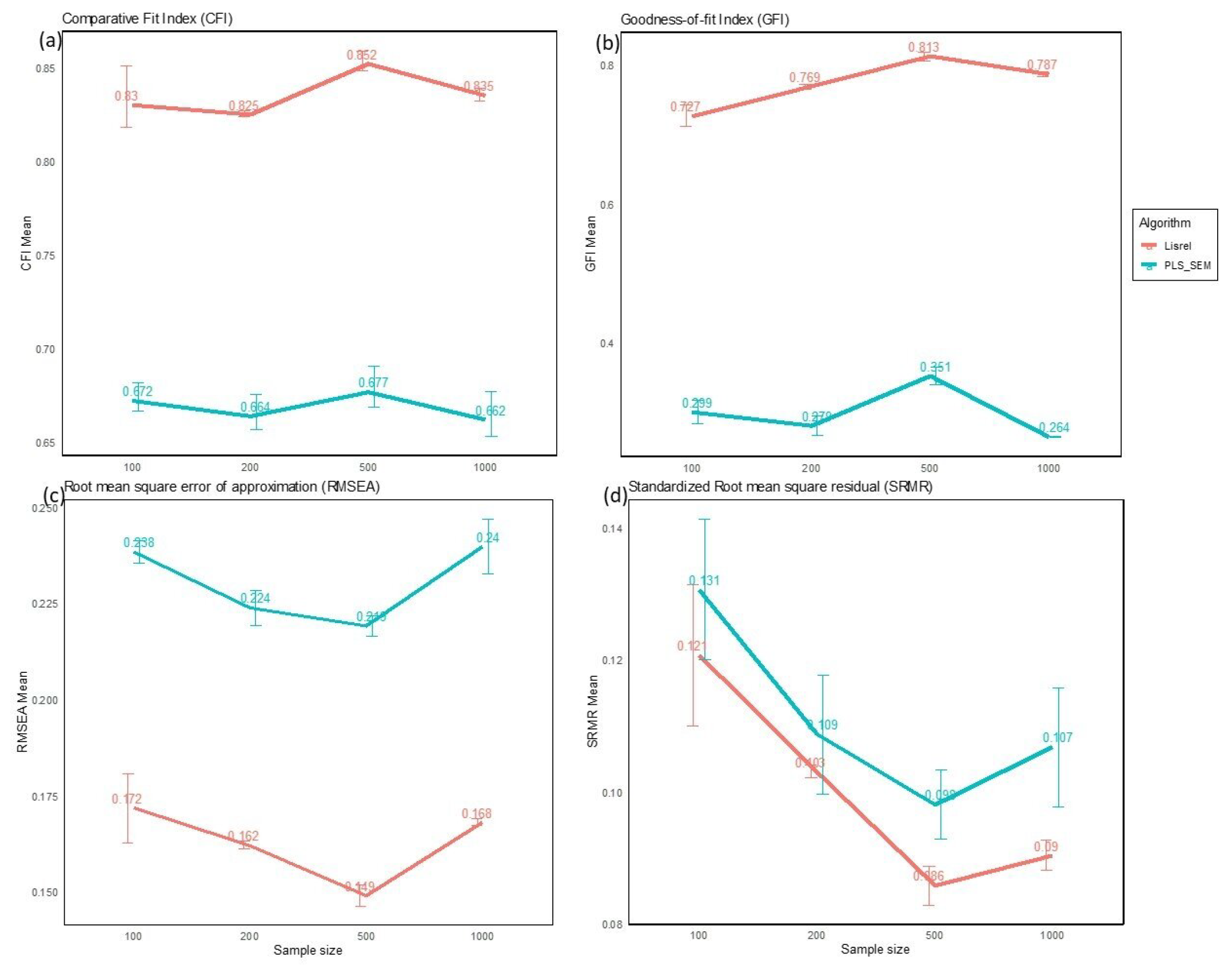
The performance of the PLS-SEM and Lisrel estimation approaches in relationship with sample size is shown in Figure 6. The average Comparative Fit Index (CFI) values show no significant tendency to increase with sample size for each estimation method. In contrast, the Goodness of Fit Index (GFI) values show a significant increase with sample size, suggesting an improvement in the proportion of information explained by the covariance matrix of the different factors in the model. The Root Mean Square Error of Approximation (RMSEA) and Standardized Root Mean Residual (SRMR) indicators decrease as the sample size increases, indicating an optimal fit of the model to the observed data. This trend is evident for both the Lisrel and PLS-SEM approaches. These results highlight that as the sample size becomes large, the models exhibit better efficiency, with a reduction in the mean difference between observed and predicted values.
Nevertheless, comparing the two approaches reveals significant differences for the four indices (Table 3). For the four performance indices, we observe a better performance of the Lisrel approach compared to PLS-SEM. Therefore, it is plausible to conclude that Lisrel stands out as the best-performing estimation method and the method performance increases with sample size.

3.2.2. Comparison Based on the Number of Indirect Effects on Model

A comparative analysis of the performance of the PLS-SEM and Lisrel algorithms, based on the number of indirect effects in the model was carried out (Figure 7). The detailed results reveal similar trends to those observed for the influence of sample size. Looking specifically at the Comparative Fit Index (CFI) and the Goodness of Fit Index (GFI), there is a slight decrease in these indices with the increasing incorporation of indirect effects, regardless of the estimation method. Indicating that as the model becomes more complex, the fit between the specified model and the observed data decreases. On the other hand, the RMSEA and SRMR indices show an opposite trend, with a significant increase of these indices when the model becomes complex, i.e., from a simple structure (without indirect effects) to a complex model (with 4 indirect effects). These observations suggest that the average deviation between observed data and predictions becomes more pronounced as model complexity increases with the inclusion of multiple indirect effects.
However, the comparative analysis between the two approaches reveals significant divergences for most of the indices (Table 4). In particular, Lisrel performs better than PLS-SEM for all performance indices. As a result, we can once again conclude that Lisrel stands out as the most effective estimation method when it comes to more complex modeling, involving the inclusion of several effects (Table 4).

3.3. Direct and Indirect Relationship between Environmental, Socio-Economic, and Climatic Variables and Incidence of COVID-19 Using the Lisrel Estimation Method

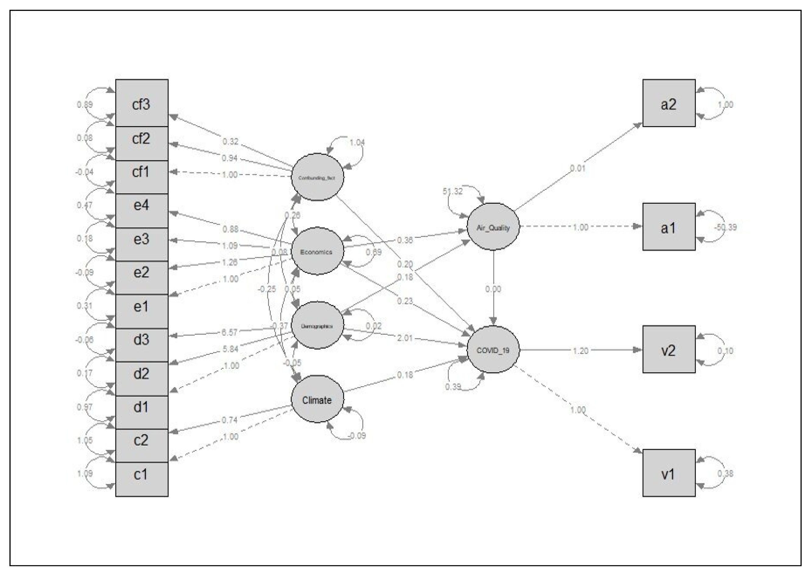
The Lisrel estimation method was the most effective. Given the effect of sample size, the most appropriate models are those with sample sizes of 500 and 1000. The analysis of the relationship between the different parameters and the effect of COVID-19 was therefore carried out using a sample of 1000. However, as the effectiveness decreases with an increasing number of indirect relationships, this evaluation was carried out based on the model with the fewest indirect relationships, namely the second model with two indirect effects. The choice of this model arises from the fact that this study seeks to highlight the direct (climate, Demographics, Air Quality, economics and confounding factors) and indirect effects (Demographics and economics factors) of various factors on the incidence of this pandemic.
A visual representation of the SEM model chosen for this study is presented as a path diagram (Figure 8). This diagram distinguishes between observed variables (framed by squares) and latent variables (represented by circles). It provides a graphical representation of structural relationships, including causality (single-headed arrows), covariance (two-headed arrows between two variables) and variances (two-headed arrows pointing to the same variable) between the observed and latent variables of the SEM.
Parameter estimates reveal that among the factors having a direct and significant influence on the incidence of COVID-19 under the control of confounding factors, there are climatic, demographic and economic factors (Table 5). Indeed, the estimated regression coefficient of climatic factors on the incidence of COVID-19 is 0.181, with significance at the 0.1% threshold (Table 5). Figure 8 indicates that an increase in humidity and a drop in temperature favor the increase of this pandemic, particularly in terms of the number of cases and deaths per 10,000 inhabitants. Similarly, the estimated direct regression coefficient of demographic factors on COVID-19 incidence is 2.01, with significance at the 0.1% level (Table 5). This suggests that an increase in factors such as the average age of the population and the proportion of people aged over 65 in a country increases the scale of this pandemic, particularly in terms of the number of cases and deaths. per 10,000 inhabitants. Also, a direct, significant and positive relationship is observed for economic factors (import and export expenditure, tourism expenditure and contribution to industrial GDP at the national level) with a coefficient of 0.231. This indicates that an increase in these factors is considered a source of the spread of this pandemic nationally. Furthermore, even if the direct correlation between atmospheric pollutants (air quality) and the incidence of COVID-19 is not significant, the results of the model reveal an indirect influence of economic factors on the incidence of COVID-19 through pollutants. Thus, air quality seems to play a media role in the complex relationship between economic factors and the dynamics of the pandemic.

4. Discussion

The assessment of data reveals varying trends in environmental parameters over three years (2019–2021) in the five main regions of Africa. Climate parameters such as temperature and humidity generally remained relatively stable over this period. The slight variations observed are consistent with the notion of a thirty-year normal in climatology, indicating that significant changes in climatic parameters necessitate a longer observation period [21]. Thus, the relative stability of climatic parameters at the regional scale suggests that differences within these regions are mainly attributable to geographical and environmental characteristics rather than short-term changes [22]. Nevertheless, these results highlight the importance of considering these regional variations in the analysis of the COVID-19 pandemic in Africa, as they may have direct implications on virus transmission, virus survival in the environment, and the respiratory health of the population.
Concerning economic parameters, countries in the northern zone, in particular, recorded higher import and export expenditures than other regions, indicating strong economic interaction with the rest of the world. Tourism spending, reflecting international mobility for leisure and travel purposes, showed a reduction in 2021 compared to 2019 across all five zones. The significant drop in tourism spending can be attributed to the massive impact of the COVID-19 pandemic on the tourism sector, resulting in travel restrictions, border closures, and health security concerns [23]. The northern zone maintained higher tourism spending, suggesting that it attracts more international travelers due to its heavy dependence on tourism [24].
Moreover, countries in the northern zone, with higher average GDP have increased industrial activity. However, industrial activities are often associated with emissions of air pollutants, which affect air quality and potentially promote the transmission of respiratory viral infections [25]. Given their economic dynamism, these northern countries appear to be more exposed to the spread of COVID-19. Their strong economic interaction, combined with intensified tourist and industrial activities that generate air pollution, may constitute additional risk factors.
Data on the number of COVID-19 cases and deaths in different African zones reinforce the importance of economic dynamics in the spread of the disease. The most affected regions in 2020 were mainly the countries of the Northern zone, highlighting a correlation between the intensity of economic exchanges and the spread of the virus. Trends in deaths also showed an increase in regions with predominant economic activity. This aligns with previous observations that economically dynamic areas face an increased risk of virus transmission, requiring appropriate health measures to contain the pandemic [26].
Comparative analyses between PLS-SEM and Lisrel approaches, both based on sample size and the number of indirect effects in the model, consistently highlight the superiority of Lisrel. Looking at the various fit indices such as CFI, GFI, RMSEA, and SRMR, Lisrel generally outperforms PLS-SEM. These findings suggest that Lisrel is more robust and better suited to modeling the relationship between variables, whether in different sample sizes or in more complex models with indirect effects. These results reinforce the conclusion that Lisrel is emerging as the preferred estimation method in these specific data analysis contexts where the aim is to confirm theories around the factors (climatic, environmental and socio-economic) that influence COVID-19 dynamics. 19. These results support the conclusions of previous studies which have specified that if the objective of the research is to test and confirm theory, then the appropriate method is CB-SEM or Lisrel over PLS-SEM [11,27].
The results of the analysis of the links between environmental and socio-economic variables and the dynamics of COVID-19 in Africa, under the control of confounding factors, from Lisrel, provide essential information. Firstly, the influence of climatic factors (temperature and humidity) highlighted in the literature [13] was confirmed by the results obtained. Furthermore, in other studies, it has been emphasized that the influence of temperature is not linear. Thus, both positive and negative correlations between temperature and the number of infections have been observed in previous studies [28,29]. They found that infections increased with increasing temperatures between 23 and 34.5 °C and decreased with temperatures between 14–23 and 34.5–39 °C. These results thus confirm the direct influence of temperature on the known spread of this pandemic.
Then, the results show that economic factors such as manufacturing GDP, import and export expenditures, tourism expenditures and demographic factors such as the average age of the population and the proportion of people aged over 65 years in a country have a significant influence on the dynamics of COVID-19. In particular, economic parameters strongly influence the number of cases and deaths per 10,000 inhabitants, with increased economic exchanges increasing the probability of transmission of the virus by human contact and by air. This confirms the observation made by [26] by specifying that the most developed countries and characterized by a strong economy are the most affected by this pandemic. Thus, countries with robust economies tend to have greater mobility of people. International trade, business travel and tourist travel are more common in these regions. This increased mobility can make it easier for the virus to spread, as more human contact means more opportunities for transmission. These results corroborate the comments made by [30] when it specifies that even if the scale of the crisis varies from one region of the world to another, all emerging and developing countries are the most vulnerable in the world made of these exogenous shocks. Concerning demographic factors (average age of the population, proportion of people aged over 65 and population density), the Lisrel model showed a significant positive influence on the number of cases, deaths per 10,000 inhabitants and the spread of COVID-19. These results confirm those obtained by [16], according to which viral spread can vary considerably from one region to another depending on population density. It is in the same sense that the [31] specifies that the low intensity of COVID-19 in Africa is mainly linked to the low population density and the lower age group. Finally, an indirect relationship was observed between the economic factors mentioned and the incidence of COVID-19 through atmospheric pollutants. This suggests that the influence of economic parameters, in particular through industrial activities, is mediated by the emission of atmospheric pollutants. However, this indirect relationship is not significant. However, the evolution of a pandemic is determined by broader societal factors, such as the capacity to control the pandemic, the functioning of the public health system, government risk management, transparency in information flows, policy adherence, and vaccination efforts [32,33]. This confirms the influence of the confounding factors noted by the model. In summary, these comprehensive analyses shed light on the multifaceted dynamics of COVID-19 in Africa, highlighting the interplay between climatic, economic, demographic and confounding factors.

5. Conclusions

Comparative analyses between PLS-SEM and Lisrel approaches, both based on sample size and the number of indirect effects in the model, consistently highlight the superiority of Lisrel. These findings suggest that Lisrel is more robust and better suited to modeling the relationship between variables, whether in different sample sizes or in more complex models with indirect effects.
The examination of data over three years (2019–2021) across African countries highlights significant trends in environmental and economic parameters linked to the spread of COVID-19. Climatically, these regions maintained relatively stable levels of temperature and humidity, suggesting that the observed short-term variations are mainly attributable to geographic and environmental characteristics. However, these regional variations play a crucial role in the transmission of the virus and the respiratory health of populations. Economically, the countries of the northern zone stand out with high import and export spending, as well as substantial tourism spending. The reduction in tourism spending in 2021, due to the massive impact of the pandemic, highlights the direct consequences on the tourism sector. Economically dynamic regions are more affected by the pandemic, which is supported by data on COVID-19 cases and deaths. The results of the Lisrel model indicate that climate, economic and demographic factors have a significant influence on the dynamics of COVID-19, confirming the preponderant role of these parameters in the spread of the virus. Based on these results, it is recommended that various African governments maintain and intensify their efforts to improve public health policies. This includes access to safe, quality, effective, efficient, accessible and affordable vaccines for the entire population. Awareness and education campaigns on the importance of vaccines and prevention measures must be implemented proactively.

Author Contributions

B.R.O.: conceptualization, Formal analysis, Writing—Review & editing. A.E.A.: Conceptualization, Formal analysis, Writing—Review & editing. K.V.S.: conceptualization, Writing—Review & editing. C.E.A.: Writing—Review & editing. J.M.K.A.: Writing—Review & editing. R.G.K.: Writing—Review & editing. All authors have read and agreed to the published version of the manuscript.

Funding

This research was funded by the EDCTP2 program supported by the European Union of funder grant number CSA2020E-3131-TEBWA. It’s also funded by the Organisation for Women in Science for the Developing World (OWSD), a program unit of UNESCO supported by the Swedish International Development Cooperation Agency of funder grant number 3240324248.

Data Availability Statement

For personal reasons, we provide the data on request.

Acknowledgments

The authors would like to thank the European & Developing Countries Clinical Trials Partnership (EDCTP), for the generous financial support given to the second author throughout the two years of his training; we would also like to thank the Organization for Women in Science for the Developing World (OWSD) for financial support to the first author.

Conflicts of Interest

The authors declare that they have no known conflict of interests or personal relationships that could have appeared to influence the work reported in this paper.

References

  1. Guihot, A.; Litvinova, E.; Autran, B.; Debré, P.; Vieillard, V. Cell-mediated immune responses to COVID-19 infection. Front. Immunol. 2020, 11, 1662. [Google Scholar] [CrossRef] [PubMed]
  2. Selma, B. L’enseignement supérieur à distance à l’ère de la COVID-19: Contraintes et obstacles à l’adaptation numérique Cas des enseignants du département de FLE des universités de l’est de l’Algérie. 2021. Available online: http://dspace.cu-barika.dz/jspui/handle/123456789/418 (accessed on 18 August 2024).
  3. Lee, C.Y.; Suzuki, J.B. COVID-19: Variants, immunity, and therapeutics for non-hospitalized patients. Biomedicines 2023, 11, 2055. [Google Scholar] [CrossRef] [PubMed]
  4. Abu-Hammad, O.; Alnazzawi, A.; Borzangy, S.S.; Abu-Hammad, A.; Fayad, M.; Saadaledin, S.; Abu-Hammad, S.; Dar-Odeh, N. Factors influencing global variations in COVID-19 cases and fatalities; a review. Healthcare 2020, 8, 216. [Google Scholar] [CrossRef] [PubMed]
  5. Honfo, S.H.; Taboe, H.B.; Kakaï, R.G. Modeling COVID-19 dynamics in the sixteen West African countries. Sci. Afr. 2022, 18, e01408. [Google Scholar] [CrossRef] [PubMed]
  6. Setti, L.; Passarini, F.; De Gennaro, G.; Barbieri, P.; Perrone, M.G.; Borelli, M.; Palmisani, J.; Di Gilio, A.; Piscitelli, P.; Miani, A. Airborne transmission route of COVID-19: Why 2 meters/6 feet of inter-personal distance could not be enough. Int. J. Environ. Res. Public Health 2020, 17, 2932. [Google Scholar] [CrossRef]
  7. Frontera, A.; Cianfanelli, L.; Vlachos, K.; Landoni, G.; Cremona, G. Severe air pollution links to higher mortality in COVID-19 patients: The “double-hit” hypothesis. J. Infect. 2020, 81, 255–259. [Google Scholar] [CrossRef]
  8. Bontempi, E. First data analysis about possible COVID-19 virus airborne diffusion due to air particulate matter (PM): The case of Lombardy (Italy). Environ. Res. 2020, 186, 109639. [Google Scholar] [CrossRef]
  9. Bourdrel, T.; Annesi-Maesano, I.; Alahmad, B.; Maesano, C.N.; Bind, M.A. The impact of outdoor air pollution on COVID-19: A review of evidence from in vitro, animal, and human studies. Eur. Respir. Rev. 2021, 30. [Google Scholar] [CrossRef]
  10. Hair, J.F., Jr.; Howard, M.C.; Nitzl, C. Assessing measurement model quality in PLS-SEM using confirmatory composite analysis. J. Bus. Res. 2020, 109, 101–110. [Google Scholar] [CrossRef]
  11. Dash, G.; Paul, J. CB-SEM vs PLS-SEM methods for research in social sciences and technology forecasting. Technol. Forecast. Soc. Chang. 2021, 173, 121092. [Google Scholar] [CrossRef]
  12. Hassan, M.M.; Kalam, M.A.; Shano, S.; Nayem, M.R.K.; Rahman, M.K.; Khan, S.A.; Islam, A. Assessment of epidemiological determinants of COVID-19 pandemic related to social and economic factors globally. J. Risk Financ. Manag. 2020, 13, 194. [Google Scholar] [CrossRef]
  13. Bukhari, Q.; Jameel, Y. Will coronavirus pandemic diminish by summer? Soc. Sci. Res. Netw. 2020, 15. [Google Scholar] [CrossRef]
  14. Yao, Y.; Pan, J.; Liu, Z.; Meng, X.; Wang, W.; Kan, H.; Wang, W. Ambient nitrogen dioxide pollution and spreadability of COVID-19 in Chinese cities. Ecotoxicol. Environ. Saf. 2021, 208, 111421. [Google Scholar] [CrossRef] [PubMed]
  15. Fattorini, D.; Regoli, F. Role of the chronic air pollution levels in the Covid-19 outbreak risk in Italy. Environ. Pollut. 2020, 264, 114732. [Google Scholar] [CrossRef] [PubMed]
  16. Villeneuve, P.J.; Goldberg, M.S. Methodological considerations for epidemiological studies of air pollution and the SARS and COVID-19 coronavirus outbreaks. Environ. Health Perspect. 2020, 128, 095001. [Google Scholar] [CrossRef]
  17. Tantrakarnapa, K.; Bhopdhornangkul, B.; Nakhaapakorn, K. Influencing factors of COVID-19 spreading: A case study of Thailand. J. Public Health 2020, 30, 621–627. [Google Scholar] [CrossRef]
  18. Sorci, G.; Faivre, B.; Morand, S. Explaining among-country variation in COVID-19 case fatality rate. Sci. Rep. 2020, 10, 18909. [Google Scholar] [CrossRef]
  19. Berrezueta, E.; Domínguez-Cuesta, M.J.; Rodríguez-Rey, Á. Semi-automated procedure of digitalization and study of rock thin section porosity applying optical image analysis tools. Comput. Geosci. 2019, 124, 14–26. [Google Scholar] [CrossRef]
  20. Atabati, A.; Adab, H.; Zolfaghari, G.; Nasrabadi, M. Modeling groundwater nitrate concentrations using spatial and non-spatial regression models in a semi-arid environment. Water Sci. Eng. 2022, 15, 218–227. [Google Scholar] [CrossRef]
  21. Bessemoulin, P.; Boucher, O. Les besoins en observations pour la climatologie. La Météorologie 2002, 2002, 36–42. [Google Scholar] [CrossRef]
  22. Haddadi, A.; Kessabi, K.; Boughammoura, S.; Rhouma, M.B.; Mlouka, R.; Banni, M.; Messaoudi, I. Exposure to microplastics leads to a defective ovarian function and change in cytoskeleton protein expression in rat. Environ. Sci. Pollut. Res. 2022, 29, 34594–34606. [Google Scholar] [CrossRef] [PubMed]
  23. El Azyzy, Y. L’incidence de la COVID-19 sur le perfectionnement des competences et l’employabilite dans le secteur du tourisme. In IX Foro Internacional de Turismo Maspalomas Costa Canaria; Universidad de Las Palmas de Gran Canaria: Las Palmas, Spain, 2021; pp. 99–115. [Google Scholar]
  24. Annexe, V. Profil Sous Régional Pour l’Afrique du Nord: Partenariats Public-privé pour une Relance Post-COVID-19 Inclusive et Verte en Afrique du Nord Sommaire. 2021. Available online: https://knowledgehub-sro-na.uneca.org/wp-content/uploads/2023/04/Profil-Afrique-du-Nord-2021-Fr.pdf (accessed on 18 August 2012).
  25. Troeger, C.; Forouzanfar, M.; Rao, P.C.; Khalil, I.; Brown, A.; Swartz, S.; Fullman, N.; Mosser, J.; Thompson, R.L.; Reiner, R.C.; et al. Estimates of the global, regional, and national morbidity, mortality, and aetiologies of lower respiratory tract infections in 195 countries: A systematic analysis for the Global Burden of Disease Study 2015. Lancet Infect. Dis. 2017, 17, 1133–1161. [Google Scholar] [CrossRef] [PubMed]
  26. Bouziane, A. L’économie mondiale et marocaine: états des lieux et analyse à l’ère de la COVID-19. Rev. Int. Du Cherch. 2022, 3. Available online: https://www.revuechercheur.com/index.php/home/article/view/479 (accessed on 18 August 2024).
  27. Hair, J.F., Jr.; Matthews, L.M.; Matthews, R.L.; Sarstedt, M. PLS-SEM or CB-SEM: Updated guidelines on which method to use. Int. J. Multivar. Data Anal. 2017, 1, 107–123. [Google Scholar] [CrossRef]
  28. Ismail, I.M.; Rashid, M.I.; Ali, N.; Altaf, B.A.S.; Munir, M. Temperature, humidity and outdoor air quality indicators influence COVID-19 spread rate and mortality in major cities of Saudi Arabia. Environ. Res. 2022, 204, 112071. [Google Scholar] [CrossRef]
  29. Prata, D.N.; Rodrigues, W.; Bermejo, P.H. Temperature significantly changes COVID-19 transmission in (sub) tropical cities of Brazil. Sci. Total Environ. 2020, 729, 138862. [Google Scholar] [CrossRef]
  30. World Bank. The Global Economic Outlook During the COVID-19 Pandemic: A Changed World; World Bank: Washington, DC, USA, 2020; Available online: https://www.worldbank.org/en/news/feature/2020/06/08/the-global-economic-outlook-during-the-covid-19-pandemic-a-changed-world (accessed on 18 August 2024).
  31. WHO. WHO Manifesto for a Healthy Recovery from COVID-19; WHO: Geneva, Switzerland, 2020; Available online: https://www.who.int/news-room/feature-stories/detail/who-manifesto-for-a-healthy-recovery-from-covid-19 (accessed on 18 August 2024).
  32. Montcho, Y.; Klingler, P.; Lokonon, B.E.; Tovissodé, C.F.; Glèlè Kakaï, R.; Wolkewitz, M. Intensity and lag-time of non-pharmaceutical interventions on COVID-19 dynamics in German hospitals. Front. Public Health 2023, 11, 1087580. [Google Scholar] [CrossRef]
  33. Montcho, Y.; Nalwanga, R.; Azokpota, P.; Doumatè, J.; Lokonon, B.; Salako, V.; Wolkewitz, M.; Glèlè Kakaï, R. Assessing the Impact of Vaccination on the Dynamics of COVID-19 in Africa: A Mathematical Modeling Study. Vaccines 2023, 11, 857. [Google Scholar] [CrossRef]
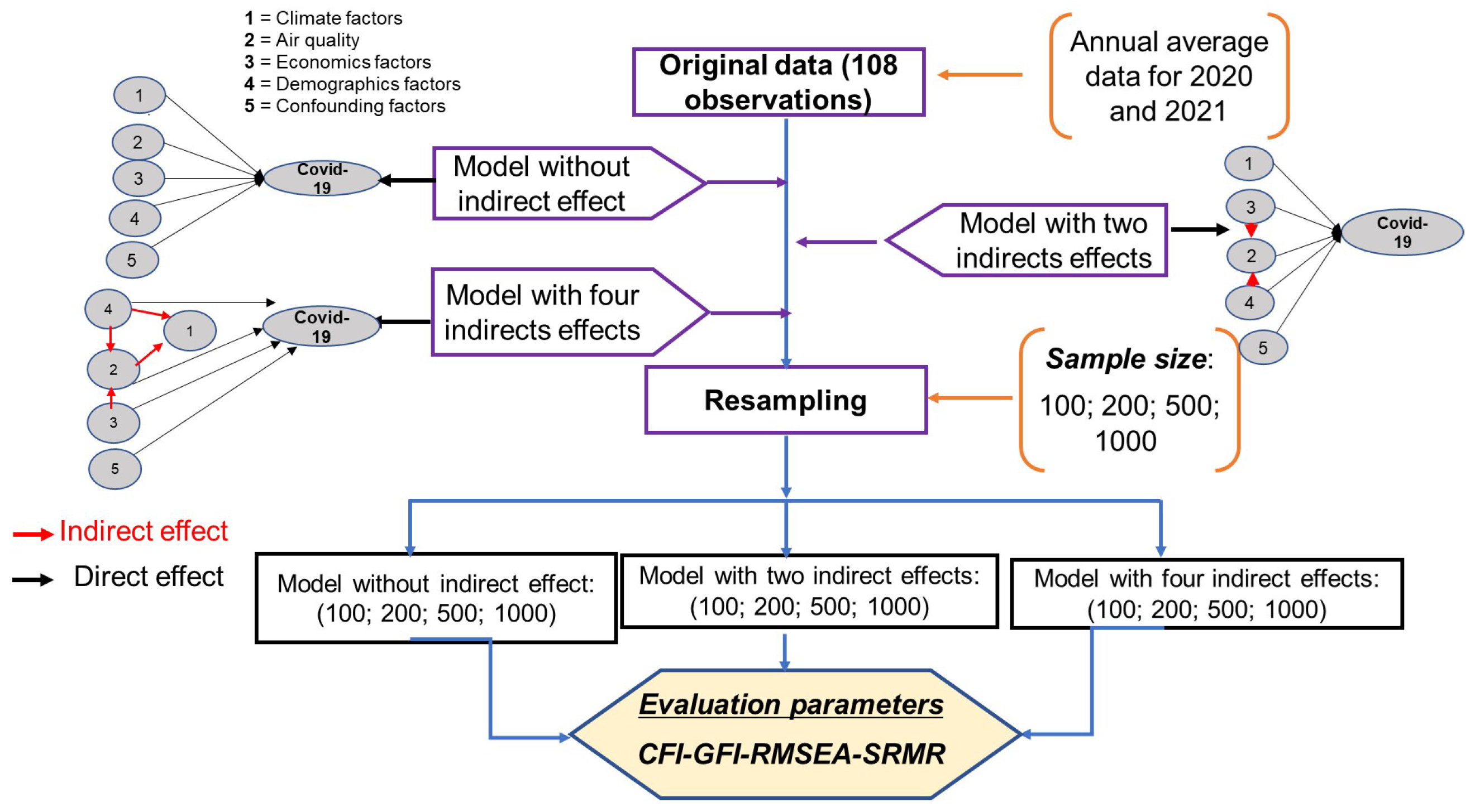
Figure 1. Flowchart of the comparative analysis of the two estimation methods.
Stats 07 00062 g001
Figure 2. Spatial patterns of climate (temperature and humidity) and environmental ( C O 2 and N O 2 emissions) factors by country. (a) Average temperature, (b) average humidity, (c) concentration of C O 2 , (d) concentration of N O 2 .
Stats 07 00062 g002
Figure 3. Spatial patterns of average economics factors by country. (a) Imports expenditure, (b) exports expenditure, (c) tourism expenditure and (d) GDP of the industrial sector.
Stats 07 00062 g003
Figure 4. Spatial analysis of average total population and proportion of seniors people by country. (a) Population average, (b) Senior population and (c) young population.
Stats 07 00062 g004
Figure 5. Spatial patterns of incidence of COVID-19 by country. (a) average incidence of cases and (b) average incidence of death due to COVID-19.
Stats 07 00062 g005
Figure 6. Performance of PLS-SEM and Lisrel based on sample size.
Stats 07 00062 g006
Figure 7. Performance of PLS-SEM and Lisrel based on number of indirect effects in model.
Stats 07 00062 g007
Figure 8. Effects of different factors on the dynamics of COVID-19 in Africa using the Lisrel approach v 1 = Incidences cases of COVID-19; v 2 = Incidences of deaths from COVID-19; c 1 = Average annual temperature (°C); c 2 = Average annual relative humidity (%); d 1 = Population density; d 2 = Proportion of senior people (more than 65 years old); d 3 = Middle age (years); e 1 = Total GDP from the industrial sector (million USD); e 2 = Total annual expenditure on imports (million USD); e 3 = Total annual expenditure on exports (million USD); e 4 = Total spending in the tourism sector per year (million USD); a 1 = The amount of carbon dioxide (kiloton) in the atmosphere; a 2 = The amount of nitrous oxide (kiloton) in the atmosphere; c f 1 = Government response index; c f 2 = Containment and health index; c f 3 = Vaccine availability.
Stats 07 00062 g008
Table 1. Data used, sources, and expected effects on the COVID-19 cases and deaths.
ParametersSourcesEffectsAuthors
Dependent variable
Covid casesWorld Health Organization (WHO).
Available online: https://covid19.who.int/data
(Accessed on 25 August 2023)
Deaths from CovidWorld Health Organization (WHO). Available online: https://covid19.who.int/data
(Accessed on 25 August 2023)
Independent variables
humidity (%)NASA. Available online: https://power.larc.nasa.gov/data
(Accessed on 2 September 2023)
+[13]
Temperature (°C)World Bank Available online: https://donnees.banquemondiale.org/
(Accessed on 3 September 2023)
+[13]
Amount of C O 2 (Kiloton)OECD (2019, 2020). Available online: https://data.oecd.org/
(Accessed on 2 September 2023); Our World in Data (2021). Available online: ourworldindata.org/
(Accessed on 2 September 2023)
+[14,15]
Amount of N O 2 (Kiloton)OECD (2019, 2020). Available online: https://data.oecd.org/
(Accessed on 2 September 2023); Our World in Data (2021).
Available online: ourworldindata.org/
(Accessed on 2 September 2023)
+[14,15]
PopulationUnited Nations. Available online: https://population.un.org/
(Accessed on 4 September 2023)
+[16]
Proportion of seniors peoples (%)Our World in Data (2021) Available online: ourworldindata.org/
(Accessed on 4 September 2023)
+[17]
Middle age (in year)Our World in Data (2021) Available online: ourworldindata.org/
(Accessed on 4 September 2023)
+[17]
GDP manufacturingFAO. Available online: https://www.fao.org/faostat/
(Accessed on 13 October 2023)
+[17,18]
TourismUNWTO Tourism Statistics Database. Available online: https://www.unwto.org/tourism
(Accessed on 15 October 2023)
+[17,18]
ImportationWorld Tourism Organization Available online: https://stats.wto.org/
(Accessed on 31 August 2023)
+[17,18]
ExportationWorld Tourism Organization Available online: https://stats.wto.org/
(Accessed on 31 August 2023)
+[17,18]
Confounding factors
Overall government response indexOxCGRT Available online: https://covidtracker.bsg.ox.ac.uk/
(Accessed on 18 March 2024)
Containment and health indexOxCGRT Available online: https://covidtracker.bsg.ox.ac.uk/
(Accessed on 18 March 2024)
Vaccine availabilityOxCGRT Available online: https://covidtracker.bsg.ox.ac.uk/
(Accessed on 18 March 2024)
+, − corresponding to the positive or negative impact of each parameter on the evolution of the pandemic respectively.
Table 2. Spatial autocorrelation index of each parameter.
FactorsMoran I StatE(X)VarStd.devp-Value
Temperature (°C)0.424 ***−0.0180.015.141.373 × 10−7
Relative humidity (%)0.568 ***−0.0180.016.5982.073 × 10−11
CO2 (Kilotons)−0.097−0.0180.01−0.9070.818
NO2 (Kiloton)−0.035−0.0180.01−0.1860.574
Import−0.012−0.0180.0060.0780.468
Export−0.048−0.0180.005−0.3960.654
Tourism spending−0.016−0.0180.0050.0270.488
Manufacturing GDP−0.086−0.0180.006−0.8720.81
Population density0.189 **−0.0180.0072.4850.007
Middle age0.311 ***−0.0180.013.7897.56 × 10−5
Individuals over ≥ 65 years old0.246 ***−0.0180.0063.2380.001
Incidence cases of COVID-190.184 ***−0.0180.0020.4980.003
Incidence deaths of COVID-190.326 ***−0.0180.0020.2011.62 × 10−5
E(x) is the mathematical expectation of Moran’s I statistic. Note: ** = p < 0.01, *** = p < 0.001.
Table 3. Multiple comparisons of the mean values of the performance indices of the two algorithms (Lisrel versus PLS) in relationship to sample size (100, 200, 500 and 1000).
SizeAlgorithmsCFIGFIRMSEASRMR
MeanSEMeanSEMeanSEMeanSE
Lisrel0.830 a0.0060.726 c0.0060.171 c0.0030.12 ab0.004
100PLS0.672 b0.0060.299 e0.0060.238 a0.0030.131 a0.004
Lisrel0.825 a0.0060.769 b0.0060.162 cd0.0030.103 bcd0.004
200PLS0.663 b0.0060.279 ef0.0060.223 b0.0030.108 bc0.004
Lisrel0.852 a0.0060.813 a0.0060.149 d0.0030.085 d0.004
500PLS0.676 b0.0060.351 d0.0060.219 b0.0030.098 cd0.004
Lisrel0.834 a0.0060.787 ab0.0060.168 c0.0030.09 cd0.004
1000PLS0.662 b0.0060.264 f0.0060.239 a0.0030.106 bc0.004
p-value 9.27 14  *** < 2 16  *** 3.72 14  ***2.22−5 ***
Comparative fit index (CFI), goodness-of-fit index (GFI), root mean square error of approximation (RMSEA) and standardised root mean square residual (SRMR). The average of each parameter was calculated over the sample size. The means of estimation methods with the same letters are not significantly different at 5%.
Table 4. Multiple comparison of the mean values of the performance indices of the two algorithms (Lisrel versus PLS) in relationship to the number of indirect effects in the model.
Indirect EffectsAlgorithmsCFIGFIRMSEASRMR
MeanSEMeanSEMeanSEMeanSE
0Lisrel0.841 a0.0060.779 a0.0180.161 b0.0050.097 a0.007
PLS0.666 b0.0060.297 b0.0180.233 a0.0050.113 a0.007
2Lisrel0.839 a0.0060.776 a0.0180.160 b0.0050.097 a0.007
PLS0.678 b0.0060.309 b0.0180.226 a0.0050.105 a0.007
4Lisrel0.826 a0.0060.766 a0.0180.166 b0.0050.104 a0.007
PLS0.662 b0.0060.288 b0.0180.230 a0.0050.114 a0.007
p-value 2.67 15  *** 6.43 15  *** 8.79 10  ***0.53
Comparative fit index (CFI), goodness-of-fit index (GFI), root mean square error of approximation (RMSEA) and standardised root mean square residual (SRMR). The average of each parameter was calculated over the number of indirect effects in the model. The means of estimation methods with the same letters are not significantly different at 5%. *** p < 0.001.
Table 5. Estimation of regression coefficients between dependent and independent variables.
EstimateStd.errZ-Valuep-Value
Direct effect on COVID-19
Climate0.1810.0483.7530.000 ***
Demographics2.0110.4244.7420.000 ***
Air Quality0.0020.0180.0710.943
Economics0.2310.0376.3240.000 ***
Confounding factors0.2010.0258.0870.000 ***
Indirect effect : Air-Quality
Demographics0.180.190.950.342
Economics0.3610.03410.660.000 ***
Performance evaluation
Number of observations1000
Test statistic15,618.67; p = 0.000 ***
RMSEA0.167
SRMR0.089
CFI0.837
GFI0.789
*** = p < 0.001.
Disclaimer/Publisher’s Note: The statements, opinions and data contained in all publications are solely those of the individual author(s) and contributor(s) and not of MDPI and/or the editor(s). MDPI and/or the editor(s) disclaim responsibility for any injury to people or property resulting from any ideas, methods, instructions or products referred to in the content.