1. Introduction
From the desire to satisfy as many human needs as possible, the natural resources offered by the Earth have been abused. Thus, the environments in which humanity lives have reached significant levels of degradation, which is why it is desired to implement a green technological process, whereby people’s well-being is not affected by the attempt to protect nature. Due to the collective responsibility for managing natural resources and ensuring their adequacy for all of humanity, a global decision has been made through the 2030 Agenda to allocate two of the 17 Sustainable Development Goals (SDGs) specifically to life below water (SDG 14) and land (SDG 15). Among the proposed marine environment are the significant reduction in pollution, the increase in resilience of these ecosystems, as well as the sustainable management of aquaculture, tourism and fishing [
1]. For life on earth, efforts are being made to combat desertification and preserve ecosystems, as well as biodiversity, together with reforestation [
2].
Although studies have shown that land use change can lead to the creation of a sustainable environment [
3], there are still researchers who raise the issue that some implications of this change are being overlooked [
4].
In the current research, the degrees of degradation of the main ecosystems in Romania are presented, together with the main causes that led to the creation of these phenomena. In order to determine the common characteristics of the counties of this country, a cluster analysis was implemented using the K-means algorithm. By means of a map illustrating the obtained classes, it is possible to note, through the lens of their geographical location, the most vulnerable or least vulnerable to damage to the environments in question.
One primary issue contributing to pollution is the utilization of single-use plastic materials, often improperly discarded, leading to environmental degradation in the areas where they accumulate. An example of this is plastic straws that affect marine biodiversity, so solutions must be found to replace them with biodegradable materials, a fact that has also been adapted in certain countries of the world [
5]. To safeguard marine biodiversity, it is essential for people to cultivate awareness and understanding of these environments. One way this can be done is through tourism, so scuba diving classes can show marine animals to locals and tourists to cultivate ocean literacy [
6]. The education system also plays an important role in teaching children about sustainability and biodiversity conservation. Thus, through implementing storytelling to students, it was demonstrated that they can improve their perspective on the human-animal relationship [
7].
Another water polluter is considered to be agricultural activities through fertilizers and the inefficient use of water sources. In order to achieve precision farming, the use of the Internet, statistical inference, machine learning and predictive analytics to maximize production while minimizing water and fertilizer consumption has been proposed [
8].
To determine the main problems, as well as ways to reduce this pollution, farmers’ opinions are very important [
9]; the directives and policies offered by the EU constitute general solutions to this problem because without a well-written legislative framework, it will be difficult for farmers to discover on their own how to combat this phenomenon [
10,
11].
Population growth, as well as the agglomeration of urban areas, leads to the degradation of the natural ecosystems that surround these zones, so the identification of measures to facilitate the water circuit in the urban environment is necessary to decelerate the degradation process of the environment, as well as of limited resources of water [
12].
Although there are enough problems to be solved with regard to life underwater and on the surface, worldwide progress has been made in preserving sustainable development and biodiversity conservation. However, progress on ocean sustainability appears to have slowed with the entry into force of the 2030 Agenda; this fact can be explained by the difference between the targets proposed for the two SDGs (14 and 15). What has also been noted is that low-income countries have lagged behind in implementing these targets, and disparities are becoming increasingly noticeable [
13].
Urban agglomerations constitute the areas with the highest exposure to air pollution, threatening not only the environment, but also human health [
14]. This pollution is due to intense industrial activity that affects the plant biodiversity of forests [
15], and one of the identified solutions is the optimal determination of the distribution of residential and industrial areas [
16].
It has also been noted that an increase in greenhouse gases leads to an increase in air temperature and thus to an increase in sea level. Global warming causes the water level to rise, which directly affects the sustainable development of humankind [
17]. These climate changes affect not only the waters but also the forests; along with industrial pollution and deforestation, global warming leads to devastating forest fires that destroy biodiversity [
18]. However, it should also be noted that the human hand can destroy these ecosystems through intentionally setting fires in the forest to facilitate land use change [
19].
The current paper aims to discuss the degree of degradation of ecosystems in Romania and illustrate the main causes that facilitated this process in raising alarm about the harmful effects of the irresponsible use of limited environmental resources.
2. Materials and Methods
For the current study, the analyzed data were extracted from the atlas written by Avram et al. [
20], in which the degrees of degradation of the main ecosystems in Romania are presented, as well as the causes that led to the appearance of these phenomena. This research aims to determine the vulnerable regions through implementing a cluster analysis using the K-means algorithm to group the counties of Romania according to the communes identified through the prism of the degrees of degradation of forests, pastures, rivers and lakes.
This algorithm is one of the most used methods for grouping objects into classes, and according to an analysis carried out from 1984 to 2021, 44,433 articles were discovered that contained variations of ”K-means” in keywords [
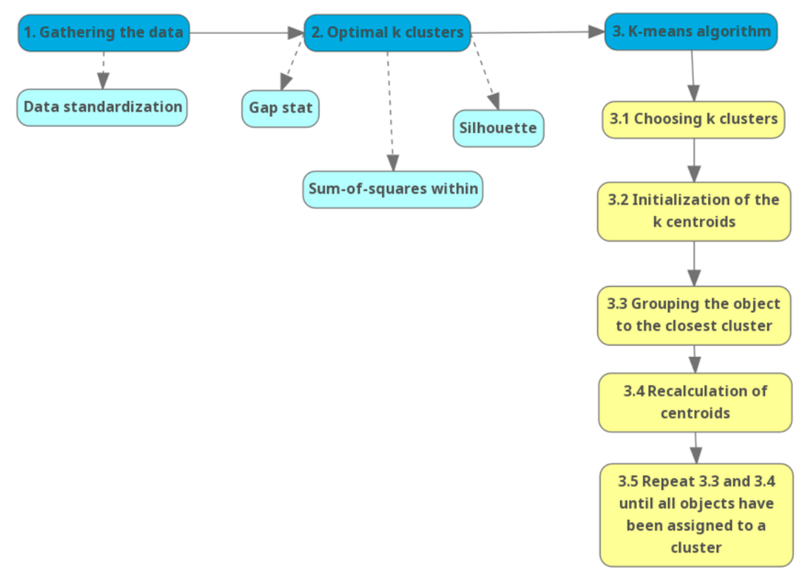
21]. The K-means algorithm assumes the initialization of a number of k objects, specified by the researcher, which are considered the initial centroids (
Figure 1). Each object in the initial set is assimilated by the nearest centroid, and the value of the centroids is recalculated whenever a new object is added to them [
22]. To determine the optimal number of clusters, the factoextra package [
23] from R was used, and the three methods applied are as follows:
silhouette [
24] (the values vary between −1 and 1, and the closer the value is to the positive value, the object is well distributed in the cluster):
where
a(
i) is the mean intra-cluster distance and
b(
i) describes the average distance to the nearest cluster.
Sum of squares within [
25]:
where
C = {
C1,
C2, …,
Cm}, m represents the number of non-overlapping clusters,
P is the optimal partition and n is the number of objects.
gap stat [
26]:
where
Wm describes the pooled sum of square within cluster around the cluster means and
E*n designates expectation under a sample of dimension
n.
3. Results
In this section, information regarding the degree of degradation of the main ecosystems identified in Romania will be presented. The section will start with a general description of the identified data, the percentage identified for each ecosystem will be detailed at the county level and the main causes that led to the creation of these phenomena will be presented. The last step consists of presenting a cluster analysis using the K-means algorithm.
3.1. Descriptive Statistics
The initial stage of the current research consists of a country-level analysis of the degree of degradation for forests, pastures, lakes and rivers. This information can be seen in
Table 1.
Based on the data presented in
Table 1, it can be noted that at the Romanian level, the mean percentage of forest degradation is 12.88%, with the percentages deviating, on average, by 11.89% from this value. The lowest degradation percentage is 5%, while the maximum percentage reaches 81%, with 50% of the counties having values that do not exceed 10%. Both skewness and kurtosis have positive values, a sign that small values are predominant, and the data series is leptokurtic. For Romania, it is noted that 40.21% of pastures are considered degraded, with the values deviating, on average, by 10.37% from this rate. In addition, half of the counties have values that exceed 40%, with the minimum degree of damage being 16%, while the maximum value reaches 70%. According to the skewness coefficient, the data series are symmetrical, a sign that the data are normally distributed around the mean, and the distribution is leptokurtic.
For Romanian waters, it can be seen that the mean degree of contamination of the lakes is 28.90%, with the percentages deviating, on average, by 20.23% from this value. The minimum percentage of degradation is 2%, while the maximum percentage is 89%, and half of the counties have values that do not exceed 28% (for this ecosystem, one county was considered to have no degradation). For rivers, the average degree of degradation is 32.14%, with the values deviating, on average, by 11.90% from this rate. It can be seen that the minimum percentage of damage is 9%, while the maximum reaches 64%, however, half of the counties have values that do not exceed 34%. From the point of view of the undetected values for skewness and kurtosis, the series is normally distributed.
3.2. The Degree of Degradation and the Main Causes
In this section, the degrees of degradation will be illustrated for the four ecosystems presented previously and also for two other new ecosystems that are found only in certain areas of the country. In addition, the main causes that led to the degradation will be described.
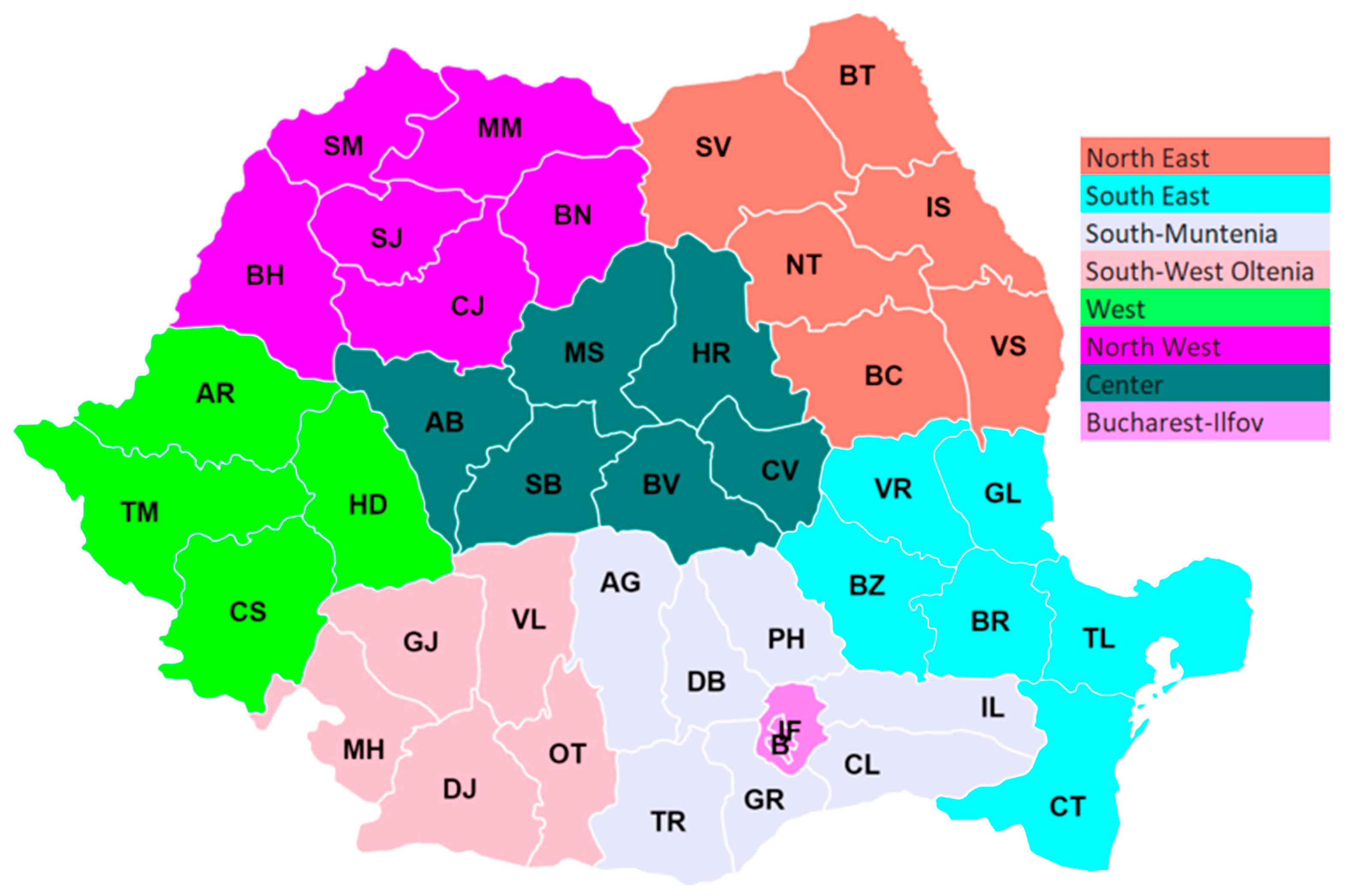
Before presenting the level of degradation encountered in the ecosystems in Romania, it must be stated that it is divided into eight development regions (
Figure 2), and the analysis is carried out via comparing the results obtained in accordance with them. The labels of the counties that make up the regions shown in
Figure 2 can be viewed via consulting
Appendix A.
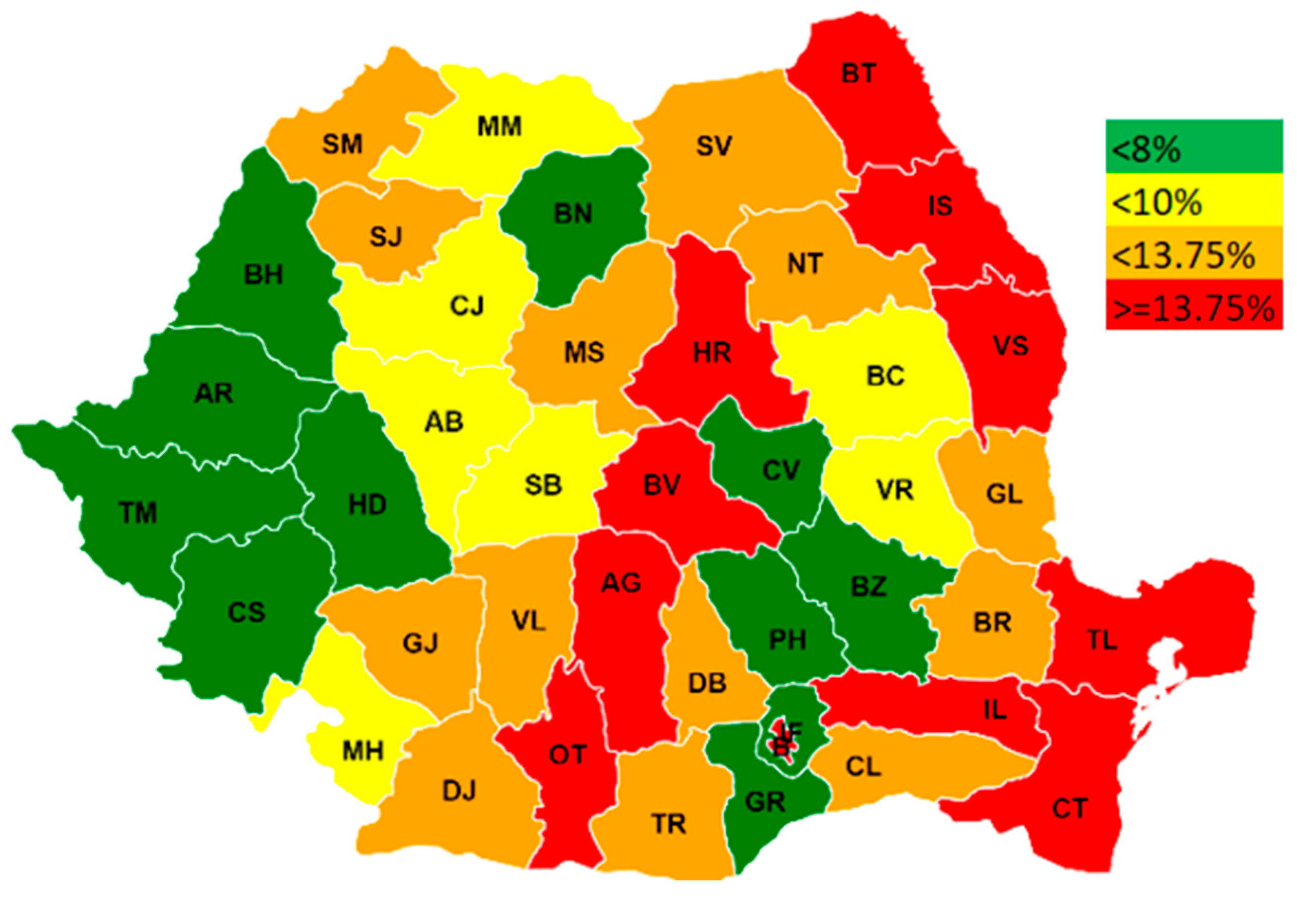
Figure 3 shows that all the counties in the Western region show low values of forest degradation percentages (below 8%). In addition, in the North-East region, half of the counties show values that equal or exceed 13.75%, and only one county has a value below 10%. For the South-West Oltenia region, only one county has a value below 10%, with all others exceeding this value.
The main causes that led to the degradation of forests are their fragmentation through the construction of roads, deforestation and wood exploitation, industrial activities (especially mining and metallurgical), agricultural activities and improper waste storage.
Figure 4 exposes that, with the exception of Ialomița county, where the percentage of degradation is below 45%, all the counties of the South-Muntenia region show deterioration rates of over 45%. For the South-East region, the percentages of degradation exceed 35%, while most counties of the Center region present rates below this value. The main reasons for grassland degradation include overgrazing, flocks, fallow, invasive vegetation and agricultural activities.
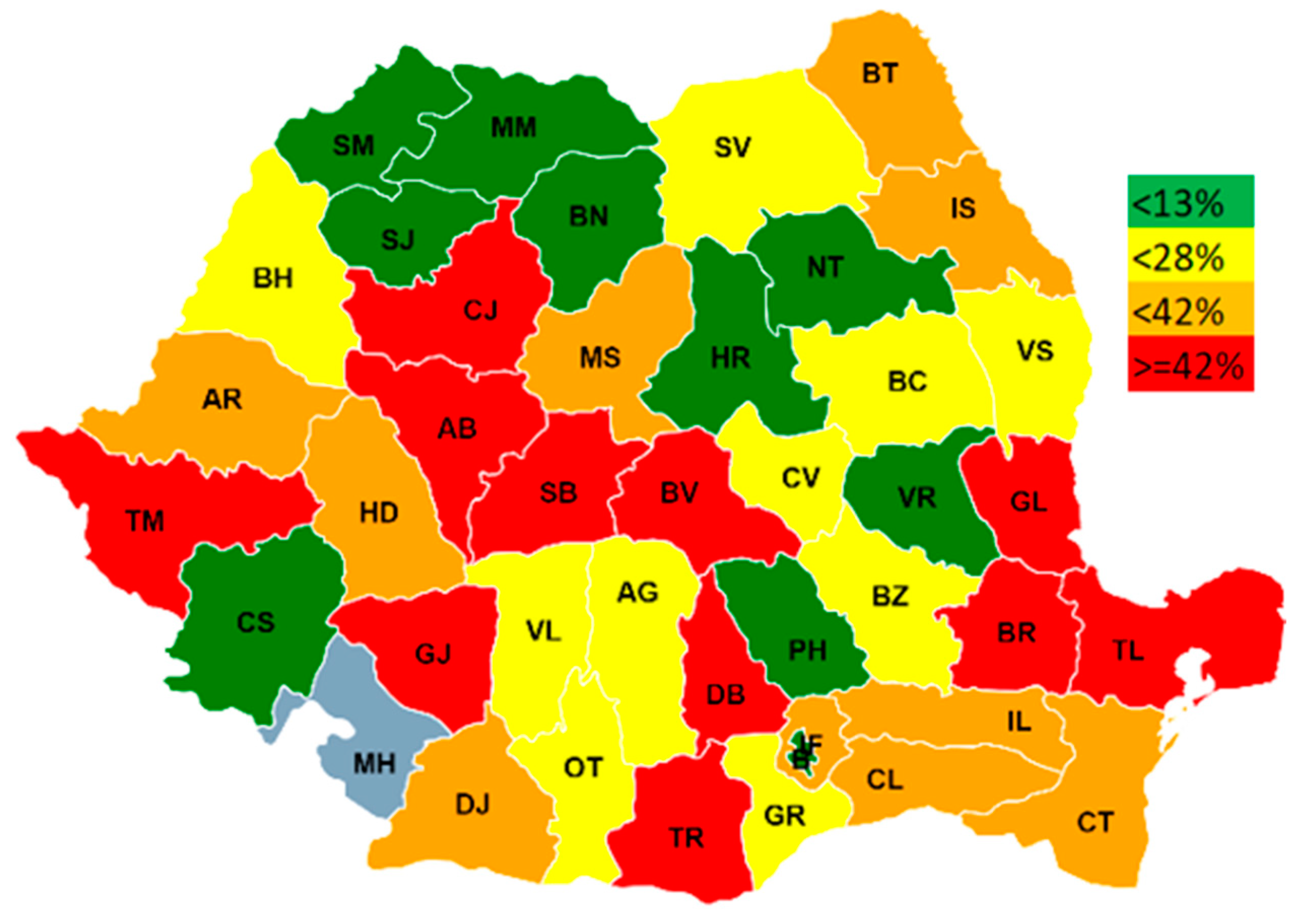
According to the map presented in
Figure 5, Mehedinți county (MH) is the only county where there are no degraded lacunar ecosystems. For the North-East region, the degradation percentages do not exceed 42%. The regions where there are the most counties with degrees of damage over 42% are Center and South-East.
Among the main causes that led to the degradation of these ecosystems are recreational activities, the high degree of vegetation cover, the discharge of wastewater, agricultural and industrial activities and transport infrastructure.
As for river ecosystems,
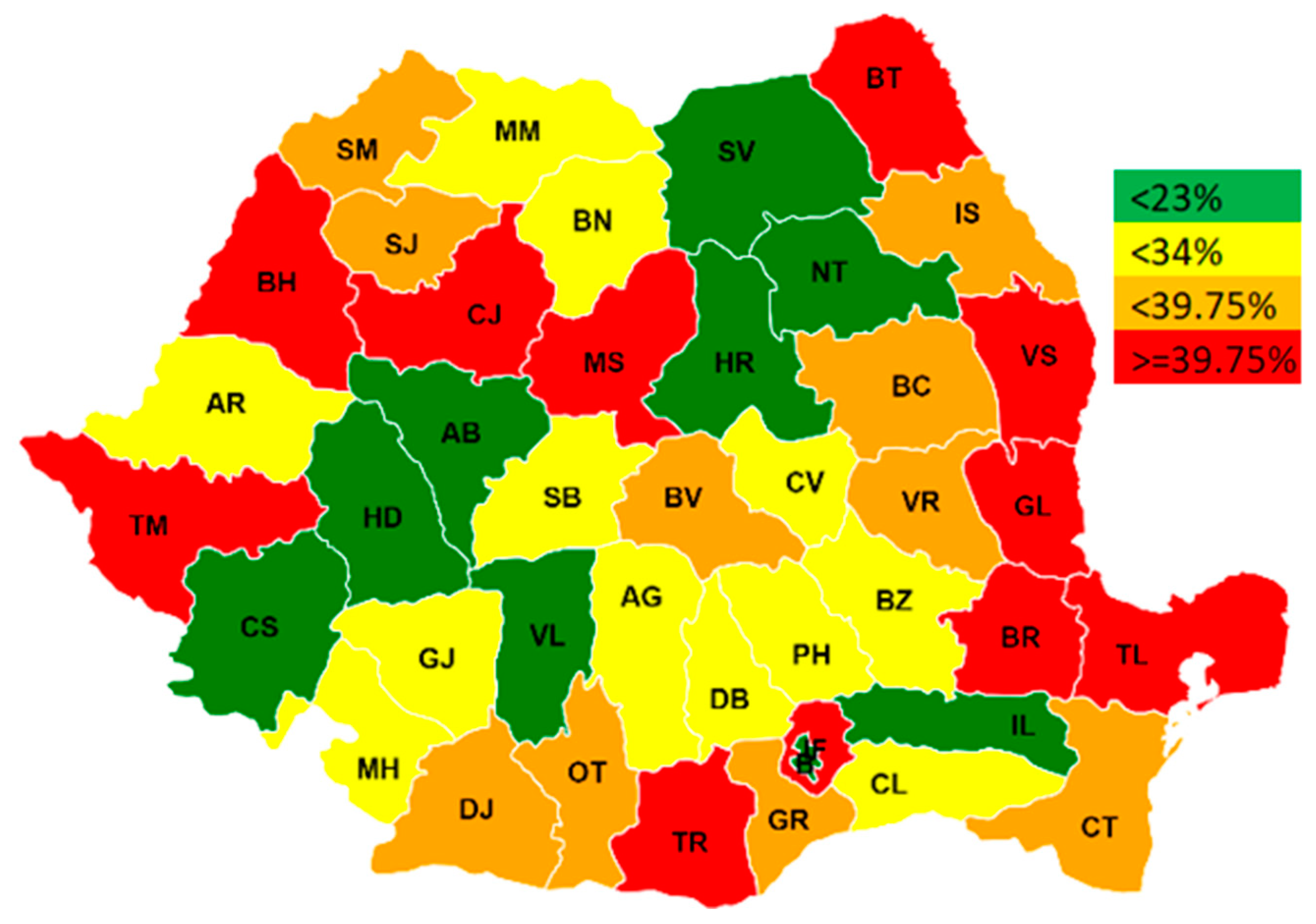
Figure 6 shows that, with the exception of Buzău (BZ) county, where the degree of degradation does not reach 34%, all other component counties of the South-East region exceed the value presented previously. For the Bucharest–Ilfov region, the contrast is significant because the capital has a percentage of degradation below 23%, while Ilfov county records a rate of deterioration of these ecosystems of over 39.75%.
Interventions in riverbeds, agricultural and industrial activities, the discharge of wastewater and the lack of water purification stations have contributed to the degradation of these ecosystems.
Degraded caves in Romania were identified only in six counties (
Table 2): Alba, Bihor, Brașov, Caraș-Severin, Hunedoara and Vâlcea, for which the percentages of deterioration vary between 11% and 100%. The main reasons why the caves reached these degrees of degradation are vandalism, excessive tourism, debris, slope collapses, crashes and deforestation.
Another type of ecosystem identified is the coastal ecosystem, present only in Constanța county, where the degree of degradation is 86%. The reasons why the coastal ecosystems in Constanta county have reached these rates of degradation are tourism activities and urbanization, industrial activities associated with the chemical sector, as well as port activities.
3.3. Cluster Analysis
For this subsection, it is desired to identify the optimal number of clusters, so that later, through applying the k-means algorithm, the counties can be classified into k chosen classes.
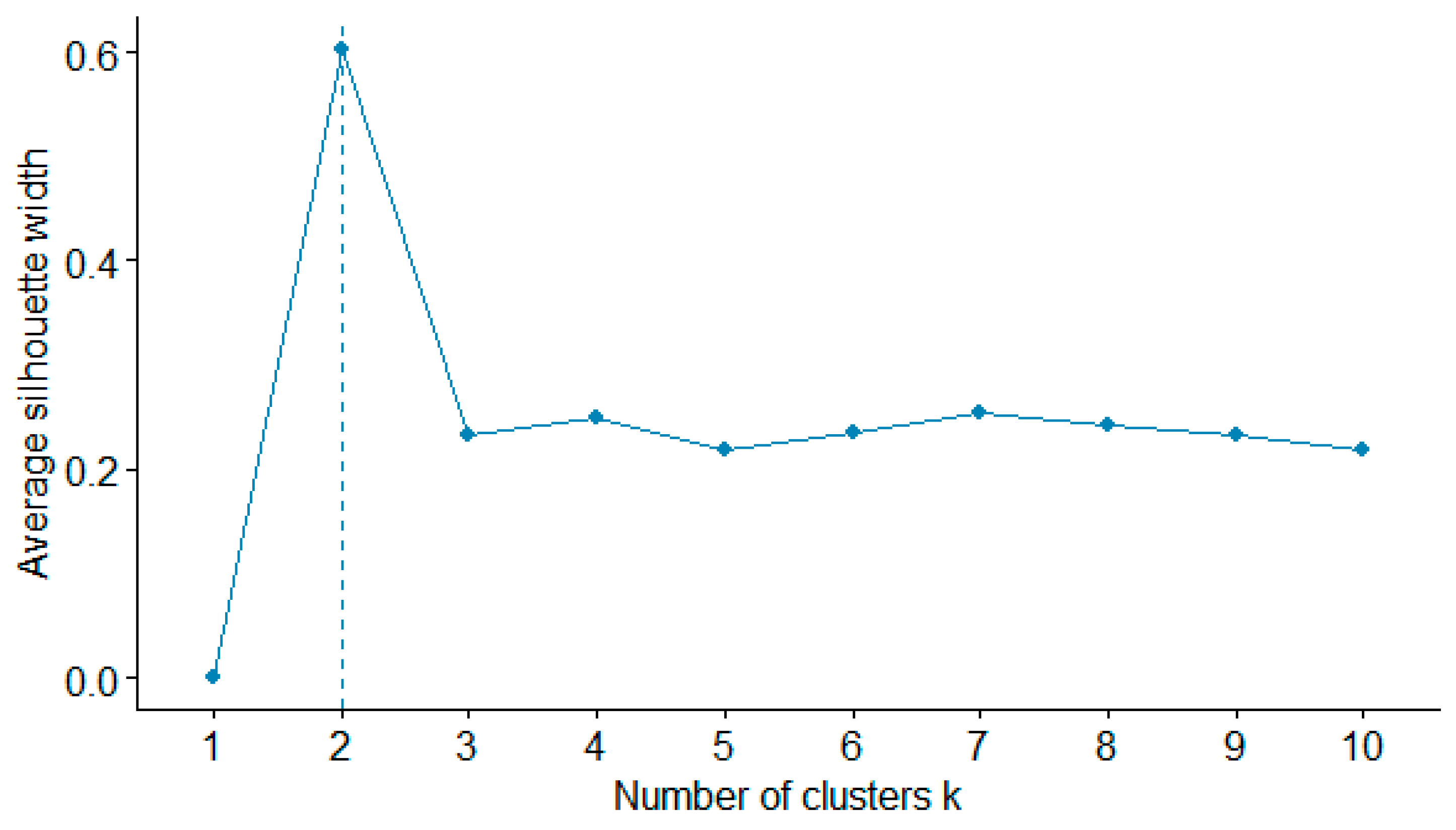
Figure 7 shows the average values of the silhouette coefficient related to a number of k clusters (from 1 to 10). It is noted that the highest value is associated with an optimal number of two clusters, and the following values in descending order are linked with four and seven classes, respectively.
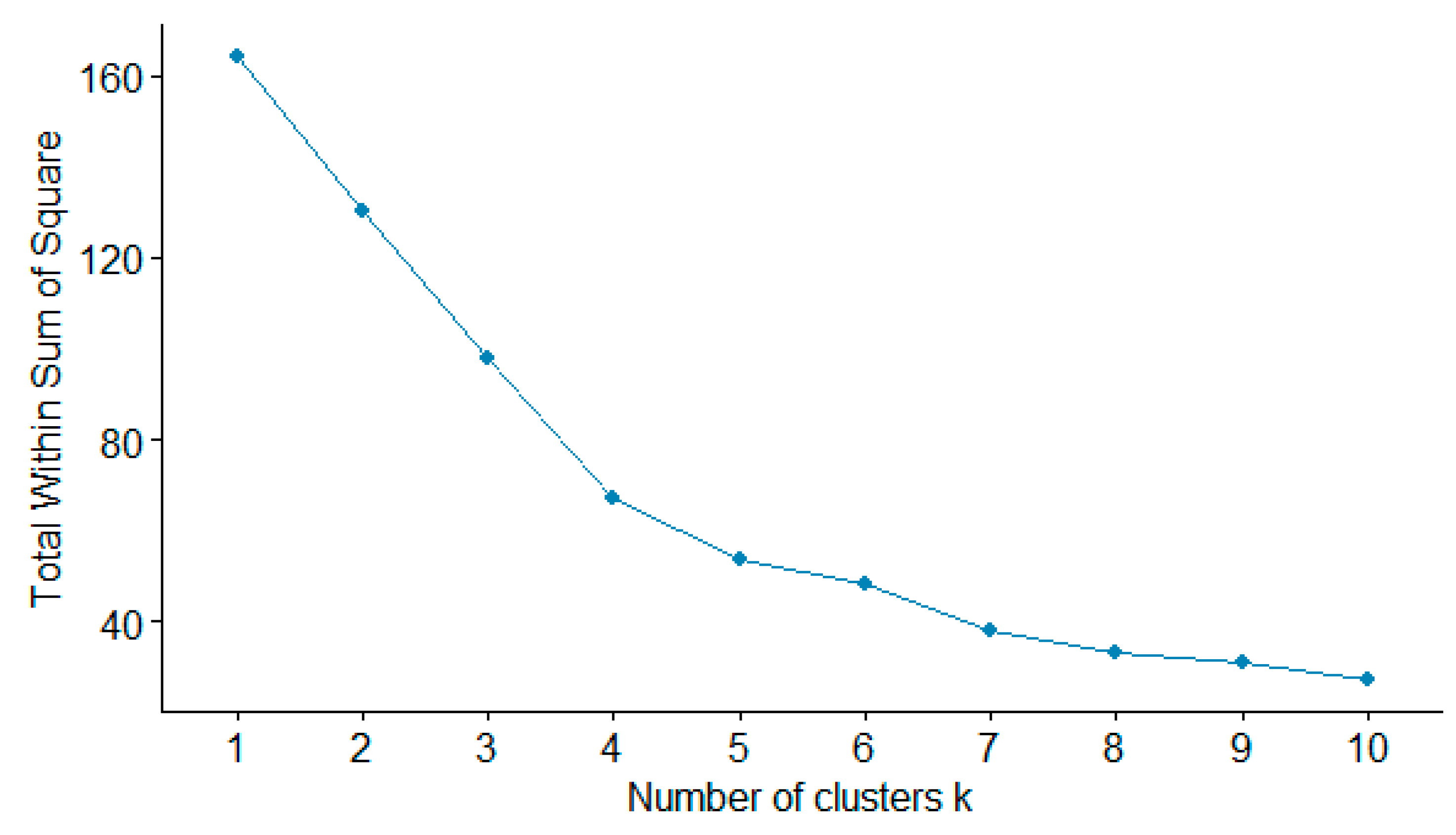
It is desirable that the intra-cluster variance be as small as possible; thus,
Figure 8 shows the related total within the sum of square values associated with different values that can define the clusters. In this case, the optimal number of classes that can be formed is four.
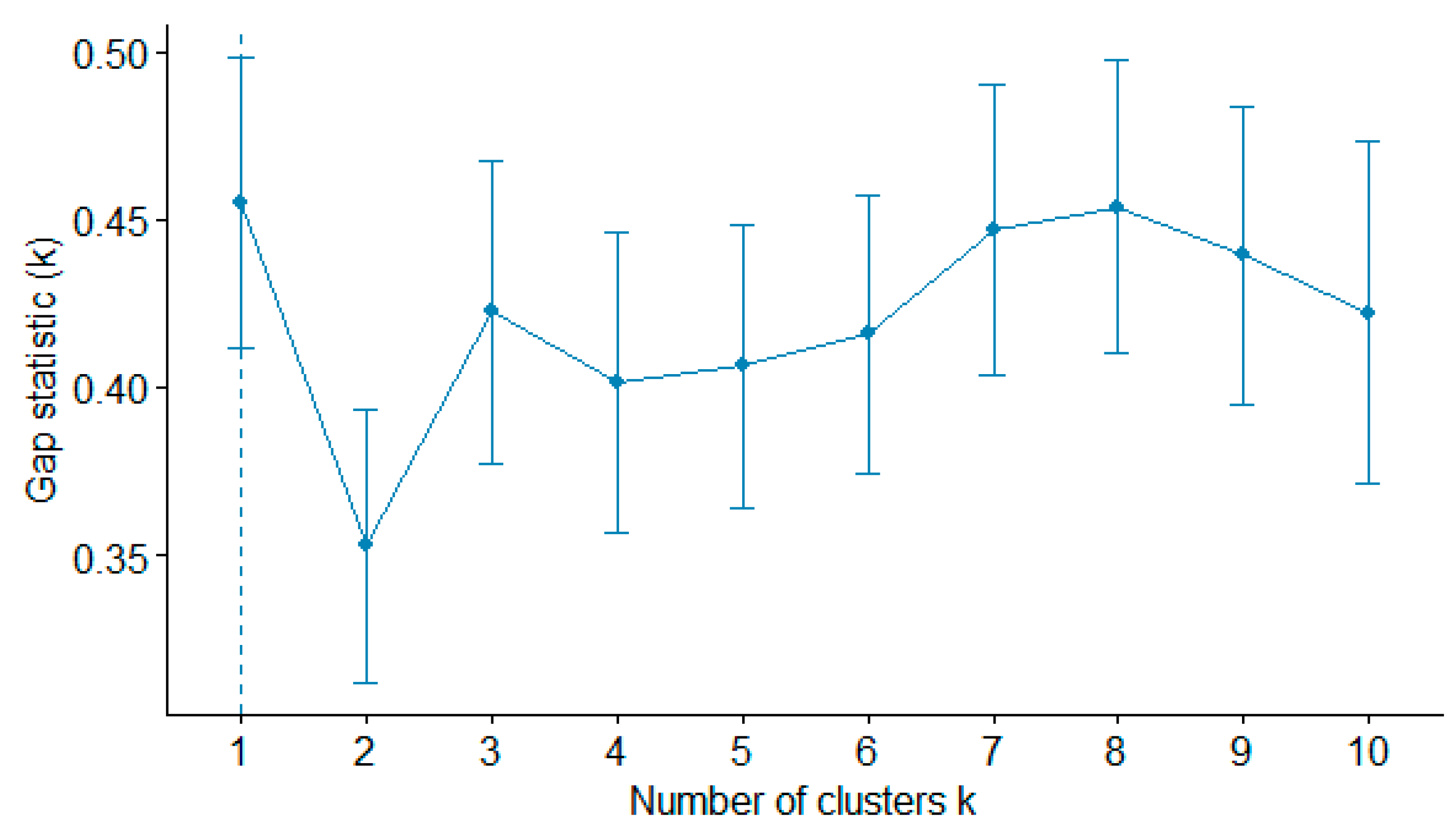
Regarding the statistical gap method, it can be seen in
Figure 9 that the optimal number proposed using the model is one cluster.
The number chosen to form the classes is four, and according to
Table 3, for this grouping, the variability between (96.61) the clusters is greater than that within (67.39) them, with their ratio being above unity (it is desirable that it be as high as possible).
For a number of two clusters, the county of Constanța (cluster 1) would have constituted a class, and all the other counties would have been grouped in a class due to the much higher percentage of forest degradation in this county (81%) compared to the others (75% of which have values below 13.75%).
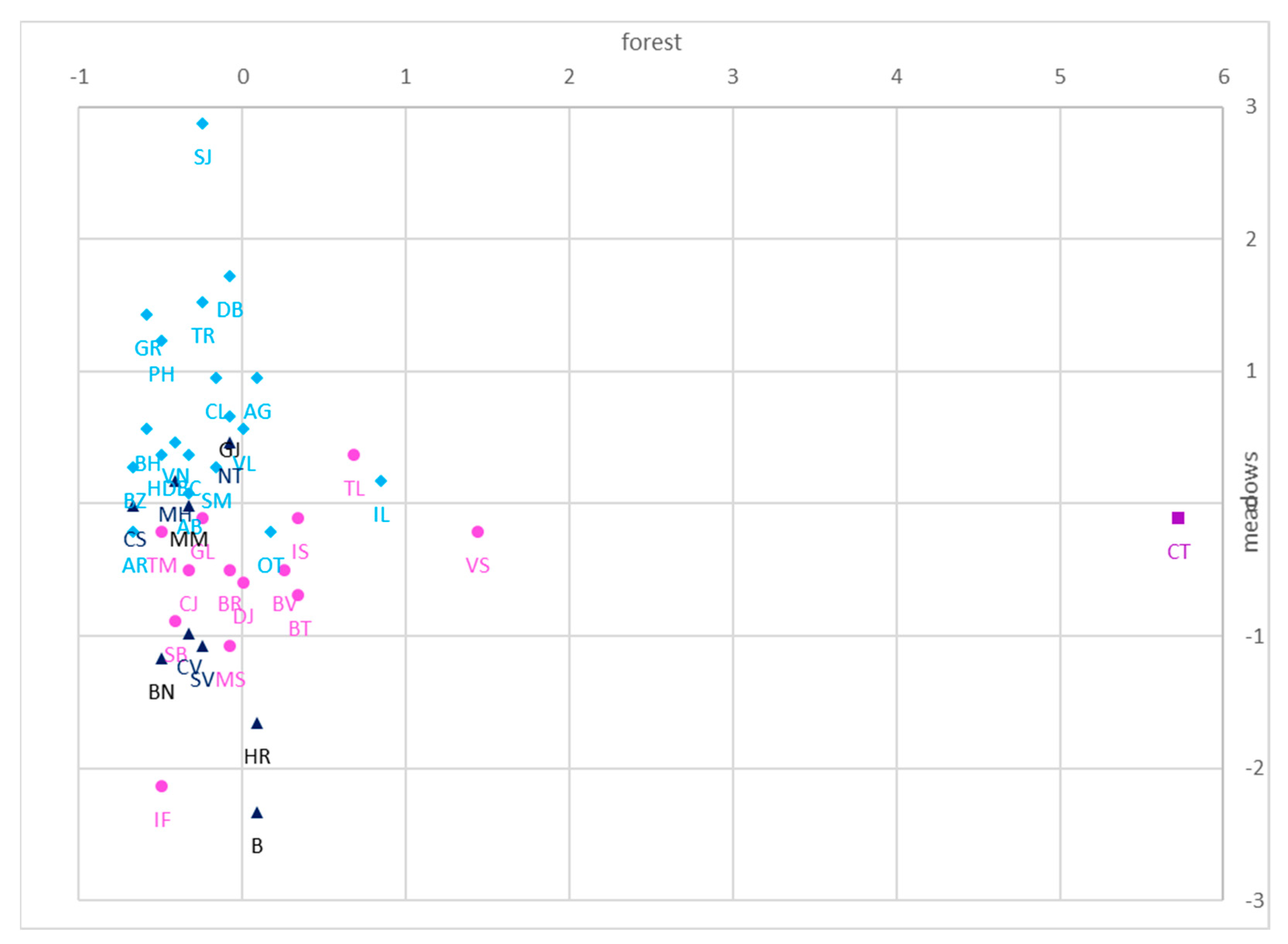
Figure 10 shows the grouping of counties in four classes corresponding to the degree of degradation of forests and pastures. The difference between Constanța and all the other counties can be clearly noted, with this having the highest value associated with the degradation of forests, as well as an average value associated with the degradation of pastures.
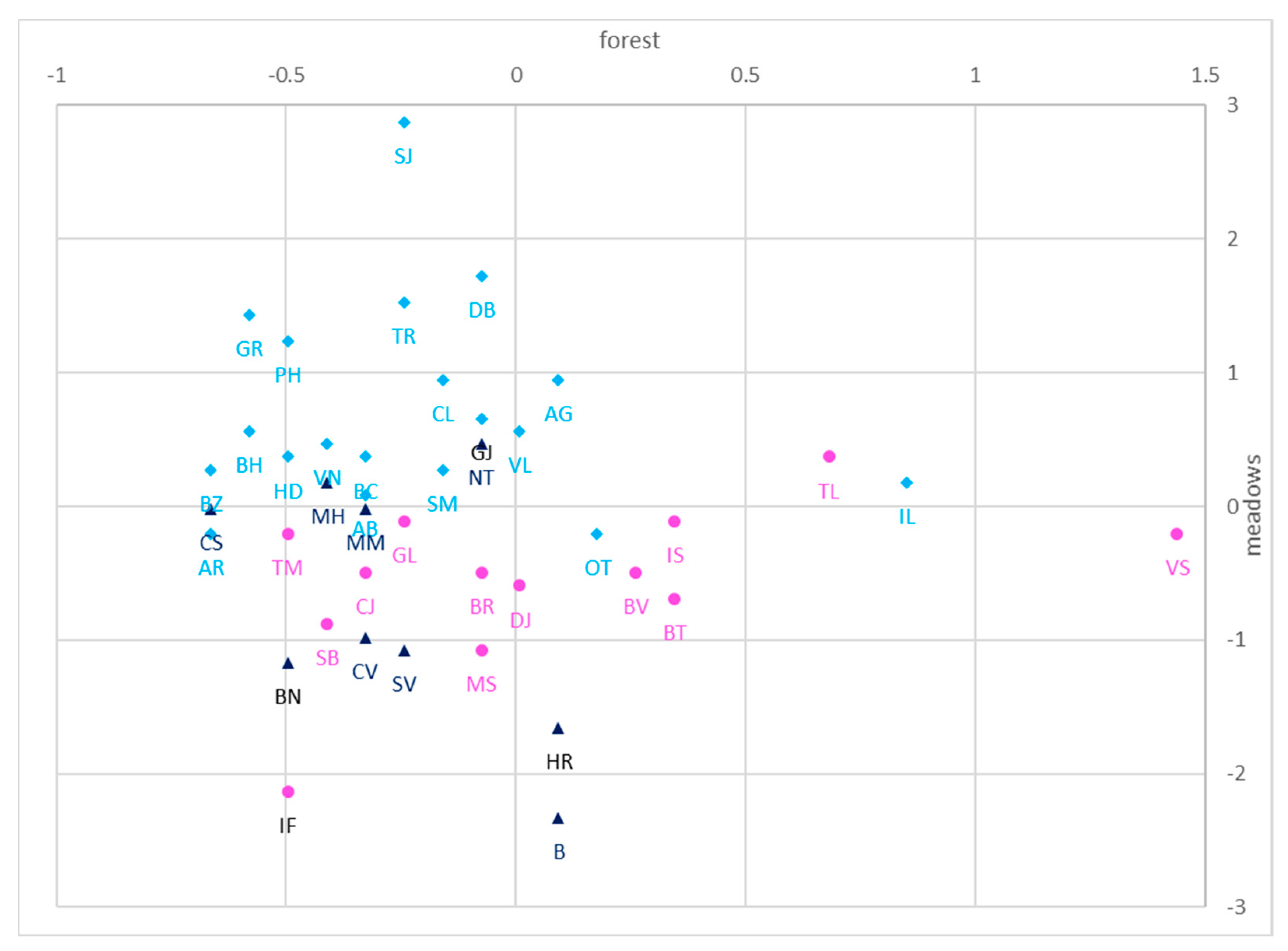
Excluding Constanța from the previous figure, the boundaries between the other three analyzed clusters can be more easily noted. Thus, from
Figure 11 it can be highlighted that most of the counties belonging to cluster 2 (BN, B, CS, CV, HR, MM, MH, NT and SV) are among the lowest recorded values of the degrees of degradation related to both analyzed ecosystems. The counties that make up cluster 3 (BT, BR, BV, CJ, DJ, GL, IS, IF, MS, SB, TM, TL and VS) are characterized by low to medium values of pasture degradation percentages, with most of them having low values of forest damage degrees, except (BV, BT, IS, TL and VS) where these percentages are significant. Cluster 4, which is composed of almost half of the country’s counties, shows average to high values in terms of the degrees of degradation of pastures, and low to medium values for forests, with the exception of AG, OT and IL.
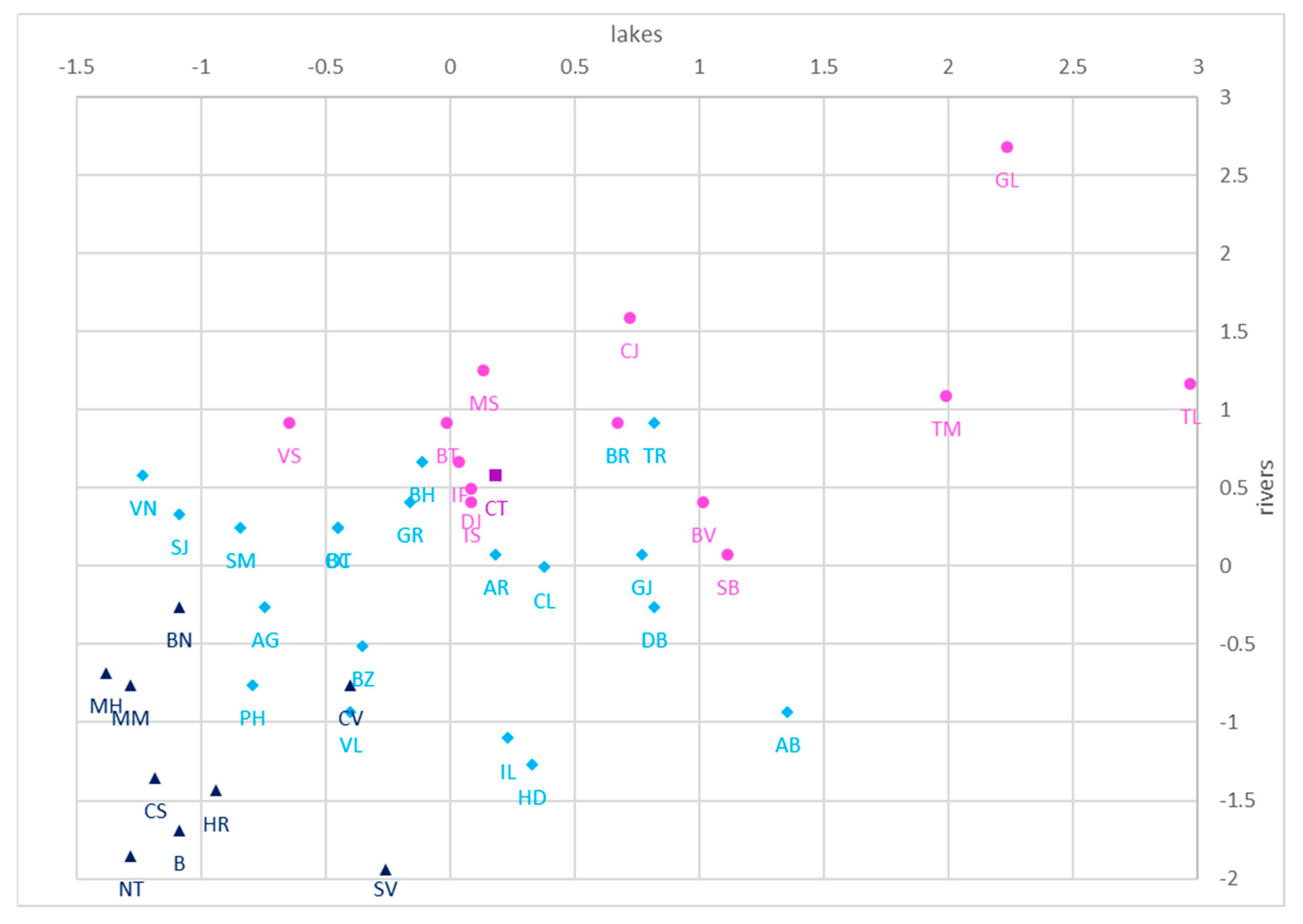
Regarding the degree of degradation of lakes and rivers, it is noted in
Figure 12 that Constanța presents an average value of degradation of rivers and low to average for lakes. The counties that define the second cluster are characterized by low values of the degrees of degradation of the two analyzed environments, while cluster 3 is distinguished by medium to high percentages of the degrees of damage to these ecosystems. Counties in the fourth cluster are described as having low to medium percentages for lake and river degradation stages.
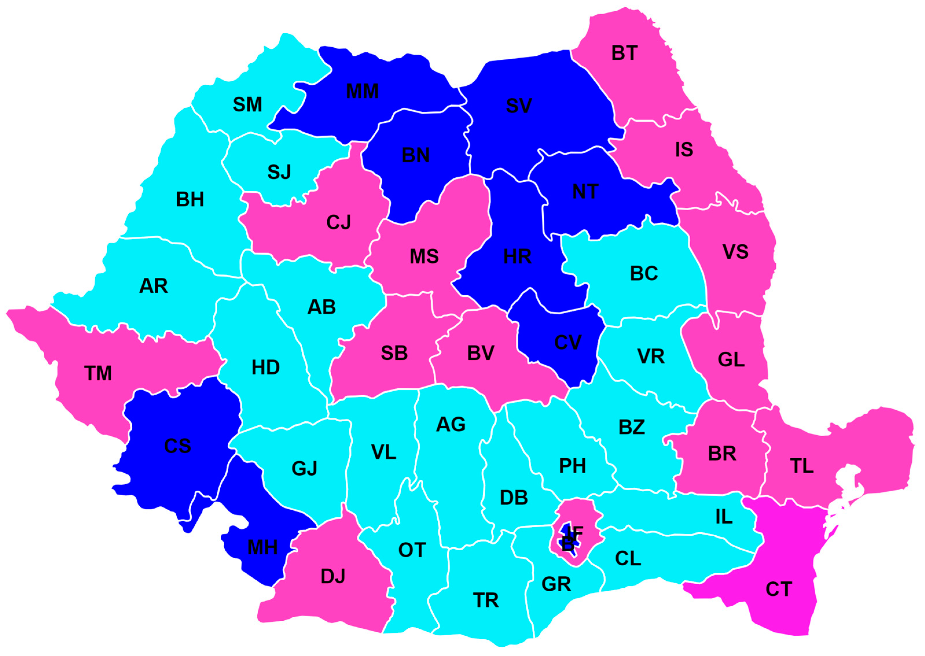
Figure 13 shows that the placement of counties in clusters does not depend much on their geographical location, although it can be seen that parts of the clusters are geographically concentrated together. Thus, cluster 2 is divided into three areas, in the central–northern part, two counties are grouped in the southwest, and Bucharest appears alone in the southeast. This cluster is characterized by the lowest percentages of degradation for all four analyzed ecosystems. Cluster 4, which is composed of approximately half of Romania’s counties, stretching from the northwest to the southeast, not including the east and the northern–central area is characterized by medium to high values of grassland deterioration, but low to medium values for the other three environments.
3.4. Economic Implications
In addition to the negative effects on the environment, the economic impact of these degradations should also be noted.
Thus,
Table 4 shows the correlations between the degrees of degradation of the analyzed ecosystems and GDP (expressed in euros per inhabitant). The orange and green colors in
Table 4 depicts a positive correlation between the implied variables, a higher intensity of the green, showing a stronger positive correlation, a lighter green a medium positive correlation, while orange shades a lower positive correlation. In the same manner, the negative correlations are depicted in dark orange and light red: the dark orange present a lower negative correlation, while the light red a medium negative correlation. A medium intensity and inverse relationship between GDP and the percentage of pasture degradation can be noted; thus, increasing the degree of pasture degradation leads to a decrease in GDP.
Table 5 shows the correlations between the percentages of ecosystem degradation and output of the agricultural ‘industry’ (million euro), and also the rate of job vacancies (from agriculture, industry and water distribution; sanitation, waste management and decontamination activities). The vacancy rate is calculated as the ratio between the number of vacant jobs and the total number of jobs expressed as a percentage. It is noted that for all four ecosystems, an increase in the percentage of degradation leads to an increase in the output of the agricultural industry.
For the vacancy rate, an indirect and strong connection between the vacancy rate in agriculture and the percentage of pasture degradation is observed, thus, an increase in the degree of pasture degradation leads to a decrease in the vacancy rate, which is also evident in the case of rivers and lakes, but the intensity of the links is much lower. Regarding the rate of job vacancies, it is noted that an increase in the degree of forest degradation leads to a decrease in this rate, with the connection being one of medium intensity. The same principle applies to rivers. For water distribution, sanitation, waste management and decontamination activities, the rate of vacant jobs in this field decreases when the degree of pasture degradation increases, with a link of medium intensity between the two indicators.
4. Discussion
For forests in Romania, it was noted that pollution caused by industry, deforestation and the density of human habitats are some of the causes that led to the degradation of these environments. The negative technological impact on the forest-tundra ecosystem is caused by a decrease in soil invertebrates near the sources of technological pollution [
27].
It has also been shown that the presence of the metallurgical and chemical industries leads to a decrease in the diameter and height of some species of trees and shrubs, thus reducing the amount of wood that people have at their disposal [
28]. Like the case presented in the current research, according to a study carried out for another EU member state, Poland, it was noted that the urbanization of rural areas led to the reduction of land intended for agricultural activities or forests [
29].
Agricultural activities are also one of the reasons that led to the reduction of forest areas, which also affected pastures. Waters are also affected by these agricultural activities, and there is an interest from researchers in this topic for other EU countries as well [
30,
31,
32]. Industrial activities are also among the causes of water degradation, and the fashion industry is considered one of the most polluting and water consuming industries. Possible solutions to this problem are the use of biomaterials, renewable sources and recyclable processes through the implementation of sustainable production [
33].
Water resilience and pollution control [
34] are ways to manage and stop the degradation of these marine ecosystems. As global warming causes water resources to diminish, the functions of green and blue water are considered to support the life support system [
35].
Section 3.4 aimed to highlight the economic impact brought by environmental degradation. Although there is an increase in the output of the agricultural industry as a result of the increase in the degree of destruction of forests and pastures, the negative impact on GDP due to the increase in the degradation of pastures is also highlighted. Through the current research, we aim to shed light on the economic and social problems caused by the destruction of the environment, encouraging researchers to discover the problems in their own country and to discover innovative solutions to combat them. In addition, educating children in a sustainable manner will lead, over time, to avoiding such injustices brought on the environment and, implicitly, on the quality of human life.
5. Conclusions
The term sustainable development arose from humanity’s desire to balance the three great pillars: the economy, the ecology and the society. To this term is added the concept of green economy, which conveys the fact that the industrial changes that occur to help create a productive technological process from renewable sources and that confer a reduced degree of pollution must not affect human well-being. These notions arose because the earth’s limited resources no longer meet human needs. Thus, the main ecosystems that give people the resources they desperately need to live are destroyed mainly because of human activities.
Thus, in the case of Romania, the causes that contributed to the degradation of forests are the transport, mining and metallurgical industries, together with deforestation, agricultural activities and water pollution that crosses these forests. The main reasons that led to the degradation of pastures are the presence of flocks, overgrazing, null soil and invasive vegetation. Regarding the lakes, it is noted that covering them with vegetation, agricultural and industrial activities together with recreational activities have brought about their degradation. As for rivers, interventions in riverbeds, agricultural and industrial activities, and the lack of treatment plants are the major causes that led to their deterioration.
It should be noted that there are limitations to this study as well. This research is based on data provided by a single atlas, and the analysis is carried out for a single period of time and cannot be used to make subsequent comparisons with other periods. In addition, through applying the K-means algorithm, the centroids are chosen randomly and the number of classes is defined a priori, with the possibility that the chosen variant is not an optimal one. However, three distinct methods of determining the optimal number of clusters were used, and multiple models were run until the model with the highest ratio of between-to-within-class variance was determined.
The balance between the economic, ecological and social plans should be the goal. Although it has been found that an increase in the degree of degradation of ecosystems leads to an increase in income in the field of agriculture, this increase is also correlated with a decrease in GDP. In addition, environmental damage is primarily caused by pollution (in its various forms), which not only affects ecosystems but also the people who live in them. The three planes have a natural balance; although it seems that the destruction of the environment is justified by the economic component, it is observed that both the social and economic components are affected when the environment is disturbed.
