Predicting Random Walks and a Data-Splitting Prediction Region

Abstract

Perhaps the first nonparametric, asymptotically optimal prediction intervals are provided for univariate random walks, with applications to renewal processes. Perhaps the first nonparametric prediction regions are introduced for vector-valued random walks. This paper further derives nonparametric data-splitting prediction regions, which are underpinned by very simple theory. Some of the prediction regions can be used when the data distribution does not have first moments, and some can be used for high-dimensional data, where the number of predictors is larger than the sample size. The prediction regions can make use of many estimators of multivariate location and dispersion.

1. Introduction

This paper suggests prediction intervals and regions for univariate and vector-valued random walks. This section reviews random walks, renewal processes, nonparametric prediction intervals, and nonparametric prediction regions. Section 2.1 presents new nonparametric data-splitting regions.

A random walk (with drift) is defined as $Y_t=Y_{t-1}+e_t$, where $e_t$ are independent and identically distributed (iid). Suppose there is a sample $Y_1,\dots ,Y_n$ and we want a prediction interval (PI) for $Y_{n+h}$. Then, $Y_t=Y_{t-2}+e_{t-1}+e_t=Y_{t-h}+e_{t-h+1}+\cdots +e_t=Y_0+e_1+\cdots +e_t$, or $Y_{n+h}=Y_n+e_{n+1}+e_{n+2}+\cdots +e_{n+h}=Y_n+{ϵ}_{n,h}.$ Let $e_j=Y_j-Y_{j-1}$ for $j=2,\dots ,n$. Divide $e_2,\dots ,e_n$ into blocks of length h and let ${ϵ}_i$ be the sum of the $e_i$ in each block. Hence, ${ϵ}_1=e_2+\cdots +e_{h+1}$, ${ϵ}_2=e_{h+2}+\cdots +e_{2h+1}$, and ${ϵ}_i=e_{(i-1)h+2}+e_{(i-1)h+3}+\cdots +e_{(i-1)h+h+1}$ for $i=1,\dots ,m=\lfloor n/h\rfloor$. These ${ϵ}_i$ are iid from the same distribution as ${ϵ}_{n,h}$. The same decomposition can be made for a vector-valued random walk, ${\mathit{Y}}_t={\mathit{Y}}_{t-1}+{\mathit{e}}_t$, where the vectors are $p\times 1$. Thus, ${\mathit{ϵ}}_i={\mathit{e}}_{(i-1)h+2}+{\mathit{e}}_{(i-1)h+3}+\cdots +{\mathit{e}}_{(i-1)h+h+1}$ for $i=1,\dots ,m$.

The random walk can be written as $Y_t=Y_0+{\sum }_{i=1}^t{e}_i$, where $Y_0=y_0$ is often a constant. A stochastic process $\left\{N\right(t):t\ge 0\}$ is a counting process if $N\left(t\right)$ counts the total number of events that occurred in the time interval $(0,t].$ Let $e_n$ be the interarrival time or waiting time between the $(n-1)$th and nth events counted by the process, $n\ge 1$. If the nonnegative $e_i$ are iid with $P(e_i=0)<1$, then $\left\{N\right(t),t\ge 0\}$ is a renewal process. Let $Y_n={\sum }_{i=1}^n{e}_i$ denote the time of occurrence of the nth event = waiting time until the nth event. Then $Y_n$ is a random walk with $Y_0=y_0=0$. Let the expected value $E\left(e_i\right)=\mu >0$. Then $E\left(Y_n\right)=n\mu$ and the variance $V\left(Y_n\right)=nV\left(e_i\right)$ if $V\left(e_i\right)$ exists. A Poisson process with rate $\lambda$ is a renewal process where the $e_i$ are iid exponential EXP($\lambda$) with $E\left(e_i\right)=1/\lambda$. See Ross [1] for the Poisson process and renewal process. Given $Y_1,\dots ,Y_n$, then n events have occurred, and the 1-step-ahead PI denotes the time until the next event, the 2-step-ahead PI denotes the time until the next 2 events, and the h-step-ahead PI denotes the time for the next h events.

For forecasting, we predict the test data $Y_{n+1},\dots ,Y_{n+L}$ using the past training data $Y_1,\dots ,Y_n$. A large sample $100(1-\delta )\%$ prediction interval for $Y_{n+h}$ is $[L_n,U_n]$, where the coverage $P(L_n\le Y_{n+h}\le U_n)=1-{\delta }_n$ is eventually bounded below by $1-\delta$ as $n\to \infty$. We often want $1-{\delta }_n\to 1-\delta$ as $n\to \infty$. A large sample $100(1-\delta )\%$ PI is asymptotically optimal if it has the shortest asymptotic length: the length of $[L_n,U_n]$ converges to $U_s-L_s$ as $n\to \infty$, where $[L_s,U_s]$ is the population shorth: the shortest interval covering at least $100(1-\delta )\%$ of the mass.

The shorth estimator of the population shorth will be defined as follows. If the data are $Z_1,\dots ,Z_n$, let $Z_{\left(1\right)}\le \cdots \le Z_{\left(n\right)}$ be the order statistics. Let $\lceil x\rceil$ denote the smallest integer greater than or equal to x (e.g., $\lceil 7.7\rceil =8$). Consider intervals that contain c cases $[Z_{\left(1\right)},Z_{\left(c\right)}],[Z_{\left(2\right)},Z_{(c+1)}],\dots ,[Z_{(n-c+1)},Z_{\left(n\right)}]$. Compute $Z_{\left(c\right)}-Z_{\left(1\right)},Z_{(c+1)}-Z_{\left(2\right)},\dots ,Z_{\left(n\right)}-Z_{(n-c+1)}$. Then the estimator shorth(c) $=[Z_{\left(s\right)},Z_{(s+c-1)}]$ is the interval with the shortest length.

For a large sample $100(1-\delta )\%$ PI, the nominal coverage is $100(1-\delta )\%$. Undercoverage occurs if the actual coverage is below the nominal coverage. For example, if the actual coverage is 0.93 when $n=100$, then for a large-sample 95% PI, the undercoverage is 0.02 = 2%. Suppose the data $Z_1,\dots ,Z_n$ are iid, and a large sample $100(1-\delta )\%$ PI is desired for a future value $Z_f$. The shorth(c) interval is a large sample $100(1-\delta )\%$ PI if $c/n\to 1-\delta$ as $n\to \infty$, which often has the asymptotically shortest length. Frey [2] showed that for large $n\delta$ and iid data, the shorth(${\displaystyle k_n=\lceil n(1-\delta )\rceil }$) prediction interval has maximum undercoverage $\approx 1.12\sqrt{\delta /n}$, and uses the large sample $100(1-\delta )\%$ PI shorth(c) =

$$[L_n,U_n]=[Z_{\left(s\right)},Z_{(s+c-1)}]\mathrm{with}$$

(1)

$$c=min(n,\lceil n[1-\delta +1.12\sqrt{\delta /n}]\rceil ).$$

The shorth PI (1) often has good coverage for $n\ge 50$ and $0.05\le \delta \le 0.1$, but the convergence of $U_n-L_n$ to the population shorth length $U_s-L_s$ can be quite slow. Under regularity conditions, Grübel [3] showed that for iid data, the length and center of the shorth($k_n$) interval are $\sqrt{n}$-consistent and $n^{1/3}$-consistent estimators of the length and center of the population shorth interval, respectively. The correction factor also increases the length of PI (1). Einmahl and Mason [4] provides large sample theory for the shorth under slightly milder conditions than Grübel [3]. Chen and Shao [5] shows that the shorth PI converges to the population shorth under mild conditions for ergodic data.

The large sample $100(1-\delta )\%$ shorth PI (1) may or may not be asymptotically optimal if the $100(1-\delta )\%$ population shorth is $[L_s,U_s]$ and the cumulative distribution function (cdf) $F\left(x\right)$ does not strictly increase in intervals $(L_s-ϵ,L_s+ϵ)$ and $(U_s-ϵ,U_s+ϵ)$ for some $ϵ>0$. Suppose that Y has a probability mass function (pmf) $p\left(0\right)=0.4,p\left(1\right)=0.3,p\left(2\right)=0.2,p\left(3\right)=0.06$, and $p\left(4\right)=0.04$. Then, the $90\%$ population shorth is [0,2] and the $100(1-\delta )\%$ population shorth is [0,3] for $(1-\delta )\in (0.9,0.96]$. Let $W_i=I(Y_i\le x)=1$ if $Y_i\le x$ and 0, otherwise. The empirical cdf

$${\widehat{F}}_n\left(x\right)=\frac{1}{n}\sum _{i=1}^{n}I(Y_i\le x)=\frac{1}{n}\sum _{i=1}^{n}I(Y_{\left(i\right)}\le x)$$

is the sample proportion of $Y_i\le x$. If $Y_1,\dots ,Y_n$ are iid, then for fixed x, $n{\widehat{F}}_n\left(x\right)\sim binomial(n,F\left(x\right)).$ Thus, ${\widehat{F}}_n\left(x\right)\sim AN(F\left(x\right),F\left(x\right)(1-F\left(x\right))/n)$ where $AN$ stands for asymptotically normal. For the Y with the above pmf, ${\widehat{F}}_n\left(2\right)\stackrel{P}{\to }0.9$ as $n\to \infty$ with $P({\widehat{F}}_n\left(2\right)<0.9)\to 0.5$ and $P({\widehat{F}}_n\left(2\right)\ge 0.9)\to 0.5$ as $n\to \infty$. Hence, the large sample 90% PI (1) will be [0,2] or [0,3] with probabilities → 0.5 as $n\to \infty$ with an expected asymptotic length of 2.5 and expected asymptotic coverage converging to 0.93. However, the large sample $100(1-\delta )\%$ PI (1) converges to [0,3] and is asymptotically optimal with asymptotic coverage 0.96 for $(1-\delta )\in (0.9,0.96).$

To describe the Olive [6] nonparametric prediction region, Mahalanobis distances will be useful. Let the $p\times 1$ column vector T be a multivariate location estimator, and let the $p\times p$ symmetric positive definite matrix $\mathit{C}$ be a dispersion estimator. Then the ith squared sample Mahalanobis distance is the scalar

$$D_i^2=D_i^2(T,\mathit{C})=D_{{\mathit{w}}_i}^2(T,\mathit{C})={({\mathit{w}}_i-T)}^T{\mathit{C}}^{-1}({\mathit{w}}_i-T)$$

(2)

for each observation ${\mathit{w}}_i,$ where $i=1,\dots ,n$. Notice that the Euclidean distance of ${\mathit{w}}_i$ from the estimate of center T is $D_i(T,{\mathit{I}}_p)$, where ${\mathit{I}}_p$ is the $p\times p$ identity matrix. The classical Mahalanobis distance $D_i$ uses $(T,\mathit{C})=(\overline{\mathit{w}},\mathit{S})$, the sample mean, and sample covariance matrix, where

$$\overline{\mathit{w}}=\frac{1}{n}\sum _{i=1}^n{\mathit{w}}_i\mathrm{and}\mathit{S}=\frac{1}{n-1}\sum _{i=1}^n({\mathit{w}}_i-\overline{\mathit{w}}){({\mathit{w}}_i-\overline{\mathit{w}})}^T.$$

(3)

Consider predicting a future test value ${\mathit{w}}_f$, given past training data ${\mathit{w}}_1,\dots ,{\mathit{w}}_n$, where ${\mathit{w}}_1,\dots ,{\mathit{w}}_n,{\mathit{w}}_f$ are iid. Prediction intervals denote a special case of prediction regions with $p=1$ so the ${\mathit{w}}_i$ are random variables.

A large sample $100(1-\delta )\%$ prediction region is a set ${\mathcal{A}}_n$, such that $P({\mathit{w}}_f\in {\mathcal{A}}_n)\ge 1-\delta$ asymptotically. A prediction region is asymptotically optimal if its volume converges in probability to the volume of the minimum volume covering region or the highest-density region of the distribution of ${\mathit{w}}_f.$

Like prediction intervals, prediction regions often need correction factors. For iid data from a distribution with a $p\times p$ nonsingular covariance matrix, it was found that the simulated maximum undercoverage of the prediction region (5) without the correction factor was about 0.05 when $n=20p$. Hence, the correction factor (4) is used to provide better coverage for small n. Let $q_n=min(1-\delta +0.05,1-\delta +p/n)$ for $\delta >0.1$ and

$$q_n=min(1-\delta /2,1-\delta +10\delta p/n),\mathrm{otherwise}.$$

(4)

If $1-\delta <0.999$ and $q_n<1-\delta +0.001$, set $q_n=1-\delta$. Let $D_{\left(U_n\right)}$ be the $100q_n$th sample quantile of the $D_i$, where $i=1,\dots ,n$.

The large sample $100(1-\delta )\%$ nonparametric prediction region for a future value ${\mathit{w}}_f$ given iid data ${\mathit{w}}_1,\dots ,{\mathit{w}}_n$ is

$$\{\mathit{z}:{(\mathit{z}-\overline{\mathit{w}})}^T{\mathit{S}}^{-1}(\mathit{z}-\overline{\mathit{w}})\le D_{\left(U_n\right)}^2\}=\{\mathit{z}:D_{\mathit{z}}^2(\overline{\mathit{w}},\mathit{S})\le D_{\left(U_n\right)}^2\}.$$

(5)

The nonparametric prediction region is a large sample prediction region if the iid ${\mathit{w}}_i$ have a nonsingular covariance matrix, and is asymptotically optimal for a large class of elliptically contoured distributions, including multivariate normal distributions with nonsingular covariance matrices. Regions with smaller asymptotic volumes can exist if the distribution is not elliptically contoured. From Olive [7], simulated coverage was often near the nominal for $n\ge 20p$, but simulated volumes behaved better for $n\ge 50p$. The shorth PIs do not need the mean or variance of the $e_t$ to exist.

There are many prediction intervals and regions in the literature. See Beran [8], Fontana, Zeni, and Vantini [9], Guan [10], Olive [11], Steinberger and Leeb [6], Tian [7], Nordman [12], and Meeker [13], for references. The new prediction regions can be used for distributions that do not have an expected value if appropriate $(T,\mathit{C})$ is used, e.g., $(T,\mathit{C})=(\mathrm{MED}\left(\mathit{W}\right),{\mathit{I}}_p)$, where $\mathrm{MED}\left(\mathit{W}\right)$ is the coordinate-wise median. Olive [14] and Lei et al. [15] use data splitting to obtain prediction intervals for the multiple linear regression model.

Prediction regions have some nice applications besides prediction. Applying a prediction region to data generated from a posterior distribution provides an estimated credible region for Bayesian Statistics. See Chen and Shao [5]. Certain prediction regions applied to a bootstrap sample result in a confidence region. See Rajapaksha and Olive [16], Rajapaksha [17], and Olive [18]. Mykland [19] converts prediction regions into investment strategies.

New data-splitting prediction regions that do not need the nonsingular covariance matrix to exist are provided in Section 2.1, Section 2.2 describes the prediction intervals and regions for the random walk, while Section 3 presents two examples and simulations.

2. Materials and Methods

2.1. A Data-Splitting Prediction Region

Some of the new data-splitting prediction regions, described in this section, can handle ${\mathit{ϵ}}_i$ from a distribution where the population mean does not exist. Data splitting divides the training data ${\mathit{x}}_1,\dots ,{\mathit{x}}_n$ into two sets: H and the validation set V, where H has $n_H$ of the cases and V has the remaining $n_V=n-n_H$ cases $i_1,\dots ,i_{n_V}$. A common method of data splitting randomly divides the training data into two sets, H and V. Often, $n_H\approx \lceil n/2\rceil$.

The estimator $(T_H,{\mathit{C}}_H)$ is computed using dataset H. Then, the squared validation distances $D_j^2=D_{{\mathit{x}}_{i_j}}^2(T_H,{\mathit{C}}_H)={({\mathit{x}}_{i_j}-T_H)}^T{\mathit{C}}_H^{-1}({\mathit{x}}_{i_j}-T_H)$ are computed for the $j=1,\dots ,n_V$ cases in the validation set V. Let $D_{\left(U_V\right)}^2$ be the $U_V$th order statistic of the $D_j^2$, where

$$U_V=min(n_V,\lceil (n_V+1)(1-\delta )\rceil ).$$

(6)

The new large sample $100(1-\delta )\%$ data-splitting prediction region for ${\mathit{x}}_f$ is

$$\{\mathit{z}:D_{\mathit{z}}^2(T_H,{\mathit{C}}_H)\le D_{\left(U_V\right)}^2\}.$$

(7)

To show that (7) is a prediction region, suppose the ${\mathit{x}}_i$ are iid for $i=1,\dots ,n,n+1$, where ${\mathit{x}}_f={\mathit{x}}_{n+1}$. Compute $(T_H,{\mathit{C}}_H)$ from the cases in H. Consider the squared validation distances $D_k^2$ for $k=1,\dots ,n_V$ and the squared validation distances $D_{n_V+1}^2$ for case ${\mathit{x}}_f$. Since these $n_V+1$ cases are iid, the probability that $D_t^2$ has rank j for $j=1,\dots ,n_V+1$ is $1/(n_V+1)$ for each t, i.e., the ranks follow the discrete uniform distribution. Let $t=n_V+1$ and let $D_{\left(j\right)}^2$ denote the ordered squared validation distances using $j=1,\dots ,n_V$. That is, we obtain the order statistics without using the unknown squared validation distance $D_{n_V+1}^2$. Then $D_{\left(i\right)}^2$ has rank i if $D_{\left(i\right)}^2<D_{n_V+1}^2$ but rank $i+1$ if $D_{\left(i\right)}^2>D_{n_V+1}^2.$ Thus, $D_{\left(U_V\right)}^2$ has rank $U_V+1$ if $D_{{\mathit{x}}_f}^2<D_{\left(U_V\right)}^2$ and

$$P({\mathit{x}}_f\in \{\mathit{z}:D_{\mathit{z}}^2(T_H,{\mathit{C}}_H)\le D_{\left(U_V\right)}^2\})=P(D_{{\mathit{x}}_f}^2\le D_{\left(U_V\right)}^2)\ge U_V/(1+n_V)\to$$

$1-\delta$ as $n_V\to \infty$. If there are no tied ranks, then

$$P(D_{{\mathit{x}}_f}^2\le D_{\left(U_V\right)}^2)=P(D_{{\mathit{x}}_f}^2<D_{\left(U_V\right)}^2)=P(\mathrm{rank}\mathrm{of}{D}_{{\mathit{x}}_f}^2\le U_V)=U_V/(1+n_V).$$

Note that we can obtain the actual coverage $U_V/(1+n_V)$ close to $1-\delta$ for $n_V\ge 20$ for $\delta =0.05$ even if $(T_H,{\mathit{C}}_H)$ is a bad estimator. The volume of the prediction region tends to be much larger than that of the highest density region, even if ${\mathit{C}}_H$ is well-conditioned. We likely need $U_V\ge 50$ for $D_{\left(U_V\right)}^2$ to approximate the population percentile of $D_j^2={({\mathit{x}}_{i_j}-T_H)}^T{\mathit{C}}_H^{-1}({\mathit{x}}_{i_j}-T_H).$

The above prediction region coverage theory does not depend on dimension p as long as $\mathit{C}$ is nonsingular. If $\mathit{C}={\mathit{I}}_p$ or $\mathit{C}=diag(S_1^2,\dots ,S_p^2)$, then the prediction region (7) can be used for high-dimensional data, where $p>n$. Regularized covariance matrices or precision matrices could also be used.

2.2. Prediction Intervals and Regions for the Random Walk

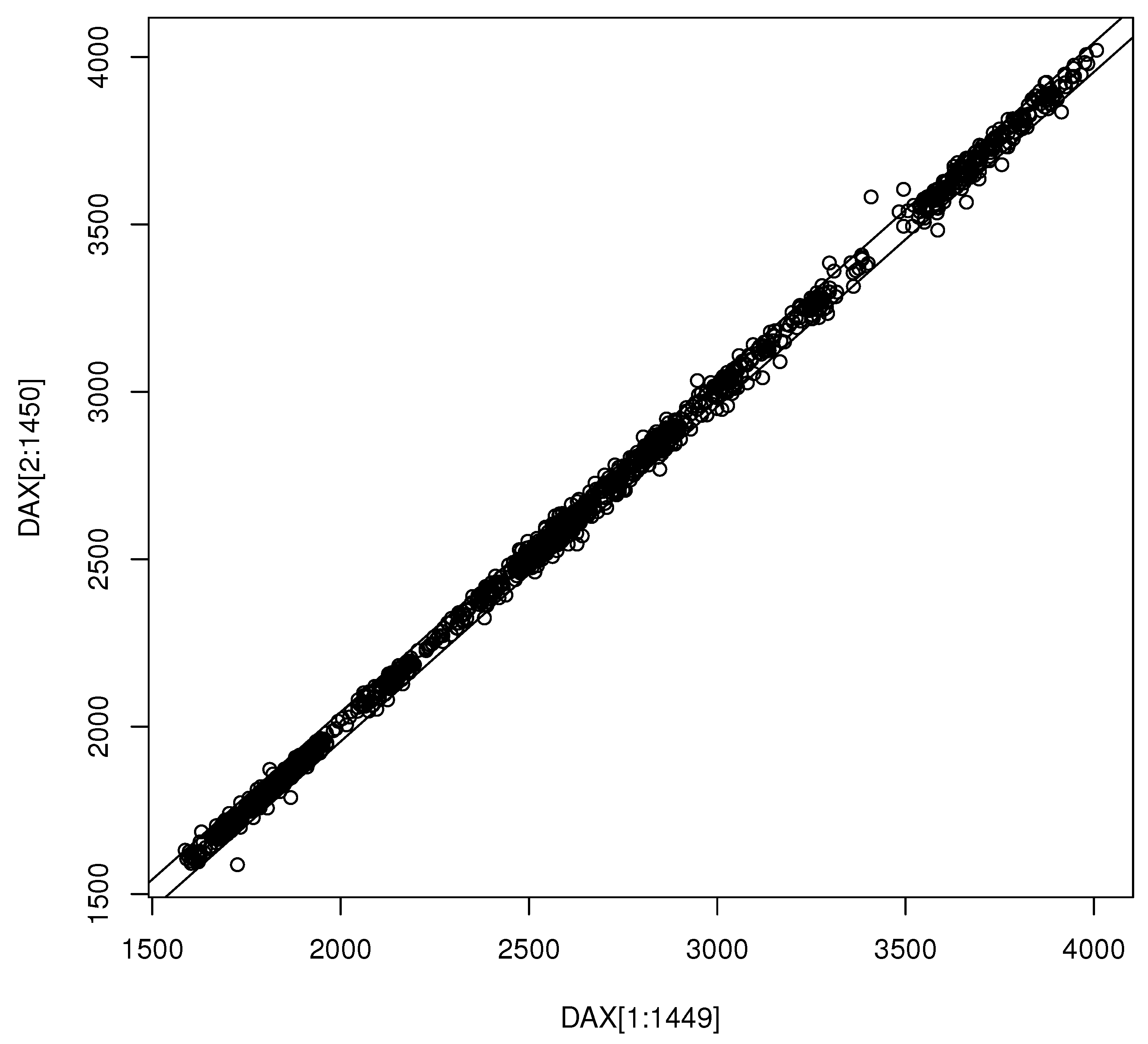
To our knowledge, asymptotically optimal nonparametric prediction intervals for the random walk have not previously been proposed. The nonparametric prediction regions described in this section may be the first ones proposed for vector-valued random walks, and are asymptotically optimal if the ${\mathit{ϵ}}_i={\mathit{ϵ}}_{i,h}$ are iid from a large class of elliptically contoured distributions. The random walk with drift is an AR(1) model with unit root and an ARIMA(0,1,0) model since $Y_t-Y_{t-1}=e_t$. Parametric prediction intervals are given by Niwitpong and Panichkitkosolkul [20] and Panichkitkosolkul and Niwitpong [21]. Wolf and Wunderli [22] considers time series prediction regions for ${(Y_{n+1},\dots ,Y_{n+L})}^T$. Parametric prediction regions have been given for vector autoregression (VAR) models. See Kim [23,24] for details and references.

The new prediction intervals and regions for random walks are simple. First, consider the random walk $Y_t=Y_{t-1}+e_t$, where $e_t$ are iid. Find the ${ϵ}_i$ for $i=1,\dots ,m=\lfloor n/h\rfloor$. Assume $n\ge 50h$ and let $[L,U]$ be the shorth(c) PI (1) for a future value of ${ϵ}_f$ based on ${ϵ}_1,\dots ,{ϵ}_m$ with $m\ge 50$. Then, the large sample $100(1-\delta )\%$ PI for $Y_{n+h}$ is $[Y_n+L,Y_n+U].$ This PI tends to be asymptotically optimal as along as $e_t$ are iid. This PI is equivalent to applying the shorth(c) PI (1) on $Y_n+{ϵ}_1,\dots ,Y_n+{ϵ}_m$.

For the vector-valued random walk ${\mathit{Y}}_t={\mathit{Y}}_{t-1}+{\mathit{e}}_t$, find ${\mathit{ϵ}}_{1,h},\dots ,{\mathit{ϵ}}_{m,h}$. The nonparametric $100(1-\delta )\%$ prediction region for a future value ${\mathit{ϵ}}_{f,h}$ is

$$\{\mathit{z}:{(\mathit{z}-\overline{\mathit{ϵ}})}^T{\mathit{S}}_h^{-1}(\mathit{z}-\overline{\mathit{ϵ}})\le D_{\left(U_m\right)}^2\}=\{\mathit{z}:D_{\mathit{z}}^2(\overline{\mathit{ϵ}},{\mathit{S}}_h)\le D_{\left(U_m\right)}^2\}$$

(8)

where ${\mathit{S}}_h$ is the sample covariance matrix of the ${\mathit{ϵ}}_{i,h}$ and $D_i^2={({\mathit{ϵ}}_{i,h}-\overline{\mathit{ϵ}})}^T{\mathit{S}}_h^{-1}({\mathit{ϵ}}_{i,h}-\overline{\mathit{ϵ}}).$ This prediction region is a hyperellipsoid centered at the sample mean $\overline{\mathit{ϵ}}$. The following large sample $100(1-\delta )\%$ prediction region for ${\mathit{Y}}_{n+h}$ shifts the hyperellipsoid (8) to be centered at ${\mathit{Y}}_n+\overline{\mathit{ϵ}}$:

$$\{\mathit{z}:{[\mathit{z}-({\mathit{Y}}_n+\overline{\mathit{ϵ}})]}^T{\mathit{S}}_h^{-1}[\mathit{z}-({\mathit{Y}}_n+\overline{\mathit{ϵ}})]\le D_{\left(U_m\right)}^2\}.$$

(9)

Since ${\mathit{Y}}_{n+h}$ has the same distribution as ${\mathit{Y}}_n+{\mathit{ϵ}}_{f,h}$, $P({\mathit{Y}}_{n+h}\in \left(9\right))=P({\mathit{ϵ}}_{f,h}\in \left(8\right))=1-{\delta }_n$, which is bounded below by $1-\delta$, asymptotically. The prediction region (9) is equivalent to applying the nonparametric prediction region (5) to ${\mathit{Y}}_n+{\mathit{ϵ}}_{1,h},\dots ,{\mathit{Y}}_n+{\mathit{ϵ}}_{m,h}$. The prediction region (9) is similar to the Olive [7] prediction region for the multivariate regression model.

Given that the ${\mathit{ϵ}}_i={\mathit{ϵ}}_{i,h}$ are iid, alternative prediction intervals and regions, such as those in Section 2.1 or Hyndman [25] for small p, could be used.

3. Results

Example 1.

Common examples of random walks are stock prices. The EuStockMarkets dataset, available from the R software, is a multivariate time series with 1860 observations on 4 variables. The observations are the daily closing prices of major European stock indices: Germany DAX, Switzerland SMI, France CAC, and UK FTSE. The data are sampled in business time, i.e., weekends and holidays are omitted. If we consider $Y_t=$ DAX, the plot of the random walk $e_t=Y_t-Y_{t-1}$ is rectangular around the $e=0$ line for cases 1–1460. Cases 1461–1800 scatter about the $e=0$ line, but have much more variability (not shown, but see Figure 9.1 in Haile [26]). Let cases 1–1450 be the training data, and let cases 1451–1460 be the test data. Figure 1 shows a plot of $Y_{t-1}$ versus $Y_t$ on the vertical axis for $t=2$ to 1450. The two parallel lines correspond to the one-step-ahead 95% prediction intervals, which cover slightly more than 95% of the training data.

Example 2.

The Wisseman, Hopke, and Schindler-Kaudelka [27] pottery data consist of a chemical analysis of pottery shards. The dataset has 36 cases and 5 groups corresponding to types of pottery shards. The variables $x_1,\dots ,x_{20}$ correspond to the $p=20$ chemicals analyzed. Consider the $n=18$ group 1 cases where the pottery shards are Arretine, which is a type of Roman pottery. We randomly select case 4 from group 1 to be ${\mathit{x}}_f$ and compute the 88.89% data-splitting prediction region with the remaining 17 cases, $n_V=8$, and $(T,\mathit{C})=(MED\left(\mathit{W}\right),{\mathit{I}}_p)$, where $MED\left(\mathit{W}\right)$ is the coordinate-wise median computed from the 9 cases in H. The cutoff is $D_{\left(U_V\right)}^2=612.2$, and $D^2\left({\mathit{x}}_f\right)=353.8$. Hence, ${\mathit{x}}_f$ is in the 88.89% prediction region. Next, we make ${\mathit{x}}_f$ equal to each of the 36 cases. Then, 8 cases ${\mathit{x}}_f$ are not in the above prediction region, including 7 of the 18 cases that are not from group 1.

The remainder of this section presents simulations for the prediction intervals and regions. More simulations and tables are presented in Haile [26]. With 5000 runs, coverages between 0.94 and 0.96 suggest that there is no reason to believe that the nominal coverage is not 0.95.

A small random walk simulation is conducted for the large-sample 95% PIs using 5000 runs with $Y_0=1$. The errors $e_t$ are iid from four distributions: (i) N(1,1), (ii) Cauchy (1,1), (iii) EXP (1), and (iv) uniform ($0,2$). Only distribution (iii) is not symmetric. We compute the h-step-ahead 95% PIs for $h=1,2,3,4=L$. We want $n\ge 50L$, but simulations may use smaller n, such as $n=25L$. The asymptotic optimal lengths are (i) 3.92, 5.54, 6.79, 7.84, (ii) 25.41, 50.82, 76.24, 101.65, (iii) 3.00, 4.72, 6.11, 7.22, (iv) 1.90, 3.11, 3.87, 4.48.

Let the population forecast error be $e\left(h\right)$. For type 1, the asymptotic optimal lengths of the large-sample 95% PIs are $3.92\sqrt{h}$, where $e\left(h\right)$∼$N(h,{\sigma }^2=h)$. For type 2, $e\left(h\right)$∼$C(h,\sigma =h)$ denotes a Cauchy distribution. For type 3, $e\left(h\right)$∼$G(h,1)$ denotes a Gamma distribution. For type 4, $e\left(2\right)$∼triangular (0,4). The distribution of the sum of n iid U (0,1) random variables is known as the Irwin–Hall distribution. See Gray and Odell [28], Marengo, Farnsworth, and Stefanic [29], and Roach [30].

The results are shown in

Table 1. Random walk 95% PI, parentheses:sd (length).

n	dist	h = 1	h = 2	h = 3	h = 4
100	N	0.9528	0.9578	0.9456	0.9220
100		4.1683 (0.3923)	6.3504 (0.9390)	7.2516 (1.2066)	7.8247 (1.4372)
100	C	0.9606	0.9656	0.9472	0.9262
100		47.33 (39.38)	1075.43 (41,234.9)	1079.36 (41,233.0)	1065.19 (41,233.7)
100	EXP	0.9552	0.9562	0.9408	0.9242
100		3.6615 (0.6325)	6.3141 (1.4891)	7.1391 (1.6336)	7.6647 (1.8121)
100	U	0.9486	0.9584	0.9408	0.9212
100		1.9023 (0.0408)	3.2878 (0.2577)	3.9791 (0.5093)	4.4074 (0.6977)
400	N	0.9526	0.9506	0.9556	0.9508
400		4.0646 (0.1868)	5.7753 (0.3813)	7.2431 (0.6028)	8.3282 (0.7921)
400	C	0.9600	0.9622	0.9654	0.9632
400		32.7277 (8.3139)	71.7138 (28.29)	133.9884 (79.20)	188.3578 (146.52)
400	EXP	0.9582	0.9598	0.9602	0.9578
400		3.3131 (0.2598)	5.1497 (0.4369)	6.7619 (0.6877)	7.9367 (0.8970)
400	U	0.9542	0.9534	0.9568	0.9558
400		1.9028 (0.0193)	3.1602 (0.1268)	4.0569 (0.2564)	4.7092 (0.3808)
800	N	0.9514	0.9520	0.9536	0.9514
800		4.0205 (0.1334)	5.7498 (0.2720)	7.0086(0.4012)	8.1579 (0.5338)
800	C	0.9520	0.9550	0.9516	0.9522
800		29.7122 (4.9301)	65.2292 (16.21)	98.9266 (31.08)	144.3277 (57.72)
800	EXP	0.9564	0.9550	0.9518	0.9596
800		3.2000 (0.1727)	5.0514 (0.3100)	6.4202 (0.4333)	7.6747 (0.5787)
800	U	0.9506	0.9522	0.9522	0.9518
800		1.9014 (0.0132)	3.1666 (0.0908)	3.9651 (0.1835)	4.6357 (0.2693)

. We roughly need $n\ge 50$ h for good coverage. Thus, $n=100$ is too small for the h-step-ahead PIs with $h=3$ and $h=4$. The Cauchy distribution requires large n before the average PI lengths get close to the asymptotically optimal lengths. Two lines are given for each distribution–sample size combination. The first line provides the coverages while the second line provides the average PI lengths with the standard deviation of the lengths in parentheses. The coverage denotes the proportion of the 5000 PIs that contain the test data case $Y_f=Y_{fi}$ for $i=1,\dots ,5000$. The last two lines of Table 1 correspond to the uniform (0,2) distribution with $n=800$. The $h=i$ label corresponds to the i-step-ahead 95% prediction interval with $i=1,2,3$ and 4. The coverages are near 0.95 and the simulated average lengths (1.9014, 3.1666, 3.9651, 4.6357) are near the asymptotically optimal lengths (1.90, 3.11, 3.87, 4.48).

A small vector-valued random walk simulation is also done for the large-sample 95% prediction regions using 5000 runs. We use distributions with nonsingular population covariance matrices. Let ${\mathit{u}}_t={(u_{t1},\dots ,u_{tp})}^T$ where $u_{ti}$ are iid from type (1) $N(1,1)$, (2) $1+t_5$, (3) EXP(1), or (4) U(0,2) distribution. Then ${\mathit{e}}_t=\mathit{A}{\mathit{u}}_t$, where $p\times p$ matrix $\mathit{A}=\left(a_{ij}\right)$ with the diagonal elements $a_{ii}=1$, and $a_{ij}=\psi$ for $i\ne j$.

Table 2. Random walk 95% prediction regions, p = 8.

n	$\mathit{\psi }$	Type	h = 1	h = 2	h = 3	h = 4
400	0	1	0.9426	0.9438	0.9370	0.9214
400	0	2	0.9490	0.9502	0.9444	0.9270
400	0	3	0.9466	0.9530	0.9476	0.9392
400	0	4	0.9416	0.9446	0.9388	0.9216
400	0.354	1	0.9514	0.9446	0.9456	0.9186
400	0.354	2	0.9450	0.9572	0.9460	0.9290
400	0.354	3	0.9556	0.9546	0.9496	0.9314
400	0.354	4	0.9416	0.9412	0.9340	0.9182
400	0.9	1	0.9484	0.9462	0.9424	0.9198
400	0.9	2	0.9524	0.9502	0.9480	0.9310
400	0.9	3	0.9482	0.9576	0.9546	0.9392
400	0.9	4	0.9458	0.9376	0.9346	0.9228
800	0	1	0.9458	0.9450	0.9460	0.9484
800	0	2	0.9516	0.9554	0.9514	0.9506
800	0	3	0.9494	0.9508	0.9480	0.9544
800	0	4	0.9432	0.9408	0.9438	0.9418
800	0.354	1	0.9456	0.9464	0.9478	0.9450
800	0.354	2	0.9474	0.9550	0.9540	0.9488
800	0.354	3	0.9534	0.9516	0.9532	0.9536
800	0.354	4	0.9494	0.9466	0.9480	0.9518
800	0.9	1	0.9436	0.9482	0.9478	0.9450
800	0.9	2	0.9500	0.9494	0.9512	0.9514
800	0.9	3	0.9552	0.9520	0.9514	0.9484
800	0.9	4	0.9474	0.9450	0.9494	0.9464
1600	0	1	0.9506	0.9516	0.9476	0.9464
1600	0	2	0.9522	0.9534	0.9532	0.9514
1600	0	3	0.9496	0.9530	0.9524	0.9522
1600	0	4	0.9418	0.9428	0.9414	0.9430
1600	0.354	1	0.9506	0.9472	0.9504	0.9502
1600	0.354	2	0.9440	0.9520	0.9488	0.9502
1600	0.354	3	0.9506	0.9572	0.9574	0.9570
1600	0.354	4	0.9488	0.9418	0.9444	0.9462
1600	0.9	1	0.9510	0.9496	0.9476	0.9458
1600	0.9	2	0.9492	0.9500	0.9532	0.9474
1600	0.9	3	0.9524	0.9558	0.9548	0.9540
1600	0.9	4	0.9450	0.9508	0.9452	0.9500

shows some results from when $p=8$, giving the coverages. We roughly need $n\ge 20ph$ to obtain good coverage near 0.95. Thus, $n=400$ is too small for $p=8$ with $h=3$ or $h=4$, although undercoverage is small for $h=3$. Note that ${\mathit{ϵ}}_t={({ϵ}_{1t},\dots ,{ϵ}_{8t})}^T$. Value $\psi =0$ makes the ${ϵ}_{it}$ uncorrelated. Increasing $\psi$ increases the correlation $\rho =cor({ϵ}_{it},{ϵ}_{jt})$, where $i\ne j$. The prediction regions are hyperellipsoids, which have volumes (not given), instead of lengths.

Simulations for the data-splitting prediction region.

The theory for the new prediction regions is simple; thus,

Table 3. Data-splitting nominal 95% prediction region.

n	p	nv	xtype	dtype	cov
50	100	20	1	1	0.9560
50	100	20	2	1	0.9466
50	100	20	3	1	0.9504
50	100	20	1	2	0.9558
50	100	20	2	2	0.9508
50	100	20	3	2	0.9522
100	100	50	1	1	0.9620
100	100	50	2	1	0.9622
100	100	50	3	1	0.9596
100	100	50	1	2	0.9638
100	100	50	2	2	0.9578
100	100	50	3	2	0.9638
100	100	25	1	1	0.9588
100	100	25	2	1	0.9658
100	100	25	3	1	0.9568
100	100	25	1	2	0.9622
100	100	25	2	2	0.9672
100	100	25	3	2	0.9662

serves more as a verification that the programs work than a test of the theory itself. See Zhang [31] for more simulations. The output variables include cov = observed coverage, up = ≈ actual coverage, and mnhsq = mean cutoff $D_{\left(U_V\right)}^2$. With 5000 runs, expect observed coverage $\in [0.94,0.96]$ if the actual coverage is close to 0.95. The random vector is $\mathit{x}=\mathit{A}\mathit{w}$, where $\mathit{x}=\mathit{w}\sim N_p(\mathbf{0},{\mathit{I}}_p)$ for xtype = 3, and $\mathit{x}\sim N_p(\mathbf{0},diag(1,\dots ,p))$ for xtype = 1. For xtype = 2, $\mathit{w}$ has the $w_i$ iid lognormal(0,1) with $\mathit{A}=diag(1,\sqrt{2},\dots ,\sqrt{p})$. The dispersion matrix types are dtype = 1 if $(T,\mathit{C})=(\overline{\mathit{x}},{\mathit{I}}_p)$ and dtype = 2 if $(T,\mathit{C})=(\mathrm{MED}\left(\mathit{W}\right),{\mathit{I}}_p)$, where $\mathrm{MED}\left(\mathit{W}\right)$ is the coordinate-wise median of the ${\mathit{x}}_i$.

When xtype = 3 and dtype = 1, $(T,\mathit{C})=(\overline{\mathit{x}},{\mathit{I}}_p)$, where ${\mathit{x}}_i\sim N_p(0,{\mathit{I}}_p)$. Then $D_{\left(U_V\right)}^2$ should estimate the population percentile ${\chi }_{p,0.95}^2$ if $n\ge max(20p,200)$ and $n_V=100$. This result did occur in the simulations.

Table 3 gives n, p, $n_V$, a number ‘xtype’ corresponding to the distribution of $\mathit{x}$, and a number ‘dtype’ corresponding to $(T,\mathit{C})$ used in the prediction region (7). High-dimensional data were used since $p\ge n$. With $n_V=20$, the actual coverage is $20/21=0.9524$; $n_V=25$ has actual coverage of $25/26=0.9615$, and $n_V=50$ has actual coverage of $49/51=0.9608$. The observed coverages are close to the actual coverages in Table 3.

4. Discussion

The new nonparametric, asymptotically optimal h-step-ahead prediction intervals for the random walk appear to perform well if $n\ge 50h$. The new nonparametric h-step-ahead 95% prediction regions for the vector-valued random walk appear to have coverages near 0.95 for $n\ge 20ph$. The new nonparametric prediction regions are fast, with simple theory, and have coverage $\ge min(n_V,\lceil (n_V+1)(1-\delta )\rceil )/(n_V+1)$.

Datasets where future data do not behave like past data are common, and then the prediction intervals and regions tend to perform poorly. In Example 1, cases 1–1460 appear to follow one random walk, while cases 1461–1800 follow another random walk with more variability.

Some prediction intervals for stochastic processes include Pan and Politis [32], Vidoni [33], and Vit [34]. Makridakis et al. [35] noted that a PI for the random walk, derived assuming normal errors, often failed to give good coverage. Pankratz [36] noted that the random walk model has been found to be a good model for many stock price time series.

Conformal prediction gives precise levels of coverage for one future observation, and prediction region (7) is a conformal prediction region that can have large volume. As an example, consider using $(T,\mathit{C})=(\mathrm{MED}\left(\mathit{W}\right),{\mathit{I}}_p)$. Then the prediction region is a hypersphere centered at the coordinate-wise median. The prediction region is good if the iid ${\mathit{w}}_i\sim N_p(\mathit{\mu },{\sigma }^2{\mathit{I}}_p)$, but if ${\mathit{w}}_i\sim N_p(\mathit{\mu },\mathbf{\Sigma })$, such that the highest density region is a hyperellipsoid tightly clustered around a vector in the direction of $\mathbf{1}={(1,1,\dots ,1)}^T$, then the prediction region (7) has large volume compared to the highest density region.

There are many methods where prediction is useful. For example, Garg, Aggarwal, et al. [37] used support vector machines while Garg, Belarbi, et al. [38] used Gaussian process regression. Olive [7] shows how to obtain prediction intervals when the model is $Y_i=m\left({\mathit{x}}_i\right)+e_i$ if the errors are iid. If heterogeneity is present, and there are enough cases ${\mathit{x}}_i$ with $\widehat{m}\left({\mathit{x}}_i\right)$ near $\widehat{m}\left({\mathit{x}}_f\right)$, we make a prediction interval using $Y_i$ corresponding to the ${\mathit{x}}_i$. Graphically, in a plot of $\widehat{m}\left({\mathit{x}}_i\right)$ versus $Y_i$ (on the vertical axis), we make a narrow vertical slice centered at $\widehat{m}\left({\mathit{x}}_f\right)$, and then make the PI from the $Y_i$ in the slice.

Plots and simulations were conducted in R. See R Core Team [39]. Programs are in the collection of functions tspack.txt. See (http://parker.ad.siu.edu/Olive/tspack.txt), accessed on 15 December 2023. Table 1 and Table 2 used functions rwpisim and rwprsim for random walk simulations. Function predsim2 simulates the data-splitting prediction region for Table 3. Function predrgn2 computes the prediction region (7) using $(T,\mathit{C})=(\mathrm{MED}\left(\mathit{W}\right),{\mathit{I}}_p).$ The pottery data are available from (http://parker.ad.siu.edu/Olive/sldata.txt), accessed on 15 December 2023.

References

1. Ross, S.M. Introduction to Probability Models, 11th ed.; Academic Press: San Diego, CA, USA, 2014. [Google Scholar]
2. Frey, J. Data-driven nonparametric prediction intervals. J. Stat. Plan. Inference 2013, 143, 1039–1048. [Google Scholar] [CrossRef]
3. Grübel, R. The length of the shorth. Ann. Stat. 1988, 16, 619–628. [Google Scholar] [CrossRef]
4. Einmahl, J.H.J.; Mason, D.M. Generalized quantile processes. Ann. Stat. 1992, 20, 1062–1078. [Google Scholar] [CrossRef]
5. Chen, M.H.; Shao, Q.M. Monte carlo estimation of Bayesian credible and HPD intervals. J. Comput. Graph. Stat. 1993, 8, 69–92. [Google Scholar]
6. Olive, D.J. Asymptotically optimal regression prediction intervals and prediction regions for multivariate data. Intern. J. Stat. Probab. 2013, 2, 90–100. [Google Scholar] [CrossRef]
7. Olive, D.J. Applications of hyperellipsoidal prediction regions. Stat. Pap. 2018, 59, 913–931. [Google Scholar] [CrossRef]
8. Beran, R. Calibrating prediction regions. J. Am. Stat. Assoc. 1990, 85, 715–723. [Google Scholar] [CrossRef]
9. Beran, R. Probability-centered prediction regions. Ann. Stat. 1993, 21, 1967–1981. [Google Scholar] [CrossRef]
10. Fontana, M.; Zeni, G.; Vantini, S. Conformal prediction: A unified review of theory and new challenges. Bernoulli 2023, 29, 1–23. [Google Scholar] [CrossRef]
11. Guan, L. Localized conformal prediction: A generalized inference framework for conformal prediction. Biometrika 2023, 110, 33–50. [Google Scholar] [CrossRef]
12. Steinberger, L.; Leeb, H. Conditional predictive inference for stable algorithms. Ann. Stat. 2023, 51, 290–311. [Google Scholar] [CrossRef]
13. Tian, Q.; Nordman, D.J.; Meeker, W.Q. Methods to compute prediction intervals: A review and new results. Stat. Sci. 2022, 37, 580–597. [Google Scholar] [CrossRef]
14. Pelawa Watagoda, L.C.R.; Olive, D.J. Comparing six shrinkage estimators with large sample theory and asymptotically optimal prediction intervals. Stat. Pap. 2021, 62, 2407–2431. [Google Scholar] [CrossRef]
15. Lei, J.; G’Sell, M.; Rinaldo, A.; Tibshirani, R.J.; Wasserman, L. Distribution-free predictive inference for regression. J. Am. Stat. Assoc. 2018, 113, 1094–1111. [Google Scholar] [CrossRef]
16. Pelawa Watagoda, L.C.R.; Olive, D.J. Bootstrapping multiple linear regression after variable selection. Stat. Pap. 2021, 62, 681–700. [Google Scholar] [CrossRef]
17. Rajapaksha, K.W.G.D.H.; Olive, D.J. Wald type tests with the wrong dispersion matrix. Commun. Stat. Theory Methods 2022. [Google Scholar] [CrossRef]
18. Rathnayake, R.C.; Olive, D.J. Bootstrapping some GLMs and survival regression models after variable selection. Commun. Stat. Theory Methods 2023, 52, 2625–2645. [Google Scholar] [CrossRef]
19. Mykland, P.A. Financial options and statistical prediction intervals. Ann. Stat. 2003, 31, 1413–1438. [Google Scholar] [CrossRef]
20. Niwitpong, S.; Panichkitkosolkul, W. Prediction interval for an unknown mean Gaussian AR(1) process following unit root test. Manag. Sci. Stat Decis. 2009, 6, 43–51. [Google Scholar]
21. Panichkitkosolkul, W.; Niwitpong, S. On multistep-ahead prediction intervals following unit root tests for a Gaussian AR(1) process with additive outliers. Appl. Math. Sci. 2011, 5, 2297–2316. [Google Scholar]
22. Wolf, M.; Wunderli, D. Bootstrap joint prediction regions. J. Time Ser. Anal. 2015, 36, 352–376. [Google Scholar] [CrossRef]
23. Kim, J.H. Asymptotic and bootstrap prediction regions for vector autoregression. Intern. J. Forecast. 1999, 15, 393–403. [Google Scholar] [CrossRef]
24. Kim, J.H. Bias-corrected bootstrap prediction regions for vector autoregression. J. Forecast. 2004, 23, 141–154. [Google Scholar] [CrossRef]
25. Hyndman, R.J. Highest density forecast regions for non-linear and non-normal time series models. J. Forecast. 1995, 14, 431–441. [Google Scholar] [CrossRef]
26. Haile, M.G. Inference for Time Series after Variable Selection. Ph.D. Thesis, Southern Illinois University, Carbondale, IL, USA, 2022. Available online: http://parker.ad.siu.edu/Olive/shaile.pdf (accessed on 15 December 2023).
27. Wisseman, S.U.; Hopke, P.K.; Schindler-Kaudelka, E. Multielemental and multivariate analysis of Italian terra sigillata in the world heritage museum, university of Illinois at Urbana-Champaign. Archeomaterials 1987, 1, 101–107. [Google Scholar]
28. Gray, H.L.; Odell, P.L. On sums and products of rectangular variates. Biometrika 1966, 53, 615–617. [Google Scholar] [CrossRef]
29. Marengo, J.E.; Farnsworth, D.L.; Stefanic, L. A geometric derivation of the Irwin-Hall distribution. Intern. J. Math. Math. Sci. 2017, 2017, 3571419. [Google Scholar] [CrossRef]
30. Roach, S.A. The frequency distribution of the sample mean where each member of the sample is drawn from a different rectangular distribution. Biometrika 1963, 50, 508–513. [Google Scholar] [CrossRef]
31. Zhang, L. Data Splitting Inference. Ph.D. Thesis, Southern Illinois University, Carbondale, IL, USA, 2022. Available online: http://parker.ad.siu.edu/Olive/slinglingphd.pdf (accessed on 15 December 2023).
32. Pan, L.; Politis, D.N. Bootstrap prediction intervals for Markov processes. Comput. Stat. Data Anal. 2016, 100, 467–494. [Google Scholar] [CrossRef]
33. Vidoni, P. Improved prediction intervals for stochastic process models. J. Time Ser. Anal. 2004, 25, 137–154. [Google Scholar] [CrossRef]
34. Vit, P. Interval prediction for a Poisson process. Biometrika 1973, 60, 667–668. [Google Scholar] [CrossRef]
35. Makridakis, S.; Hibon, M.; Lusk, E.; Belhadjali, M. Confidence intervals: An empirical investigation of the series in the M-competition. Intern. J. Forecast. 1987, 3, 489–508. [Google Scholar] [CrossRef]
36. Pankratz, A. Forecasting with Univariate Box-Jenkins Models; Wiley: New York, NY, USA, 1983. [Google Scholar]
37. Garg, A.; Aggarwal, P.; Aggarwal, Y.; Belarbi, M.O.; Chalak, H.D.; Tounsi, A.; Gulia, R. Machine learning models for predicting the compressive strength of concrete containing nano silica. Comput. Concr. 2022, 30, 33–42. [Google Scholar]
38. Garg, A.; Belarbi, M.-O.; Chalak, H.D.; Tounsi, A.; Li, L.; Singh, A.; Mukhopadhyay, T. Predicting elemental stiffness matrix of fg nanoplates using Gaussian process regression based surrogate model in framework of layerwise model. Eng. Anal. Bound. Elem. 2022, 143, 779–795. [Google Scholar] [CrossRef]
39. R Core Team. R: A Language and Environment for Statistical Computing; R Foundation for Statistical Computing: Vienna, Austria, 2020. [Google Scholar]
Figure 1. PI plot of the DAX dataset.
Stats 07 00002 g001