Abstract
In this paper, we develop a novel soft-clipping discrete beta GARCH (ScDBGARCH) model that provides an available method to model bounded time series with under-dispersion, equi-dispersion or over-dispersion. The new model not only allows positive dependence, but also negative dependence. The stochastic properties of the models are established, and these results are, in turn, used in the analysis of the asymptotic properties of the conditional maximum likelihood (CML) estimator of the new model. In addition, we apply the new model to measles infection to show its improved performance.
1. Introduction
More and more authors have underlined the importance and the common occurrence of the bounded integer-valued time series over more than two decades. McKenzie [1] proposed the binomial AR (BAR) model based on the binomial thinning operator to analyze the bounded integer-valued time series. To monitor bounded data (which increase at a certain point and then slowly decrease to the initial level), Weiß and Testik [2] further discussed the BAR model by constructing positive additive outliers; see Möller et al. [3] for its some extensions of zero inflation and Chen et al. [4] for its two types of innovative outliers. Kang et al. [5] proposed an extended binomial AR(1) model based on the generalized binomial thinning operator, which relaxes the independence assumption of the binomial thinning operator. To analyze bounded data with under-dispersion, equi-dispersion and over-dispersion, Chen et al. [6] first constructed the Conway–Maxwell–Poisson–binomial thinning operator based on the Conway–Maxwell–Poisson–binomial distribution [7], and then proposed the Conway–Maxwell–Poisson–binomial AR model. To accurately and flexibly capture the correlation structure between two random coefficients in the BAR process, Zhang et al. [8] proposed a new version of the BAR model by using the Farlie–Gumbel–Morgenstern copula, which allows both positive and negative correlations.
In fact, the volatility (especially the heteroscedasticity) is a reality for many important processes and cannot be described by the above models. Here, we take the number of districts with new cases of measles infection per week in the year 2016–2017 reported in Germany’s districts as an example and present its path in Figure 1, which shows that there seems to be more variation at the median of the time series, where the level also appears to be higher.

Figure 1.
Path of the measles infection counts.
For this purpose, Weiß and Pollett [9] considered a linear binomial ARCH(1) model, which is generalized to the pth-order case by Ristić et al. [10]. Lee and Lee [11] further discussed a version of the linear binomial ARCH(1) model with a feedback mechanism. Chen et al. [12] proposed two classes of dynamic binomial ARCH models to model time series with a finite range. Chen et al. [13] generalized the binomial ARCH model to the beta-binomial GARCH model, which allows both the conditional and marginal binomial indices of dispersion to be greater than one, i.e., data with extra-binomial variation can be more adequately captured than binomial GARCH-type models. See Liu et al. [14] for the bounded Poisson AR process and Liu et al. [15] for the novel category AR process.
However, the negative ACF cannot be achieved by the above models. To resolve this dilemma, Weiß and Jahn [16], inspired by the softplus INGARCH model [17], proposed the soft-clipping BGARCH model based on the soft-clipping function [18], i.e.,
To further investigate the soft-clipping function, we give some example of the plot of in Figure 2, when c takes the value in , From Figure 2, tends to a linear function when .
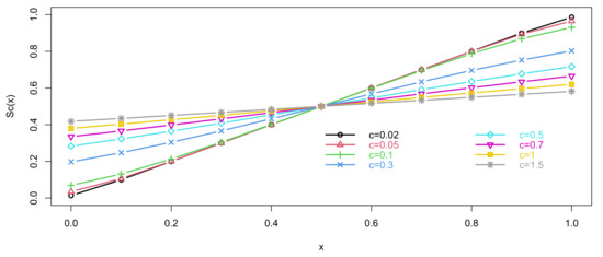
Figure 2.
Plots of the soft-clipping function.
“Although the beta-binomial distribution is very flexible with respect to its shape, it is, to a large extent focused on dealing with data sets which appear, in some way, to arise from binomial distributions but which are in fact overdispersed”, which was discussed by Turner [19]. Hence, another concern arises because beta-binomial distribution focuses on over-dispersion such that under-dispersed pseudo-binomial data sets (which are rare but do exist) cannot be analyzed by the beta-binomial GARCH-type models. To fill this gap, we proposed a new soft-clipping discrete beta GARCH (ScDBGARCH) model based on a re-scaled discrete beta binomial distribution. What is remarkable about the ScDBGARCH model is that it not only can be fitted to under-dispersed data (besides over-dispersed bounded data), but also allows negative dependence (besides positive dependence).
It is worth mentioning that the realization of negative dependence for the ScDBGARCH model is mainly due to the incorporated soft-clipping function. Another main contribution of this paper is that we establish the stochastic order of the discrete beta binomial distribution, and then discuss the stability property of the new model. In addition, we discuss the CML estimators and establish their asymptotic normality. Last but not least, we illustrate the availability and superiority in analyzing the count of districts with new cases of measles infection per week in the period of the year 2016–2017 reported in of Germany’s districts.
The paper is organized as follows. Section 2 first gives a brief review of the discrete beta distribution, then gives the definition of the soft-clipping discrete beta GARCH model and its stability properties. Conditional maximum likelihood estimation and their asymptotic properties are established in Section 3. Section 4 provides real data to show the effectiveness of the new model. Conclusions are made in Section 5. Appendix A presents some auxiliary results.
2. Model Formulation and Stability Properties
2.1. Discrete Beta Distribution
For the readers’ convenience, we first give a brief review of the discrete beta distribution, which is introduced by Turner [19].
A random variable X taking values in is said to follow a discrete beta distribution with parameters if its probability mass function of X takes the form
where
where is the predetermined upper limit of the range and or 1 is the predetermined lower limit of the range. For simplicity, we denote .
Furthermore, the probability mass function (given in (2)) of X can be rewritten as the exponential family form, i.e.,
where , , .
In fact, involving in (2) is the probability density function of the beta distribution with parameters and . By Lemma A2 in Appendix A, one can obtain the mean, variance and BID of the , if and . Similarly, the moments of can be obtained if . It is worth mentioning that and (given in Lemma A2) are precisely the mean and variance of the beta distribution with parameters and . Hence, we consider a reparameterization of the discrete beta distribution given in (2) by setting and . For simplicity, we rewrite as .
Unfortunately, the specific range of BID for the DB distribution cannot be obtained, except the case for . To solve this dilemma, we give an example of the BID in Figure 3 with and , when p and are varying from 0.1 to 0.9 with increment 0.1 and 0.1 to 8.1 with increment 0.1, respectively. See Figure 4 for .
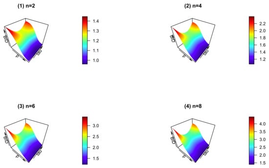
Figure 3.
Plots of the BID when .
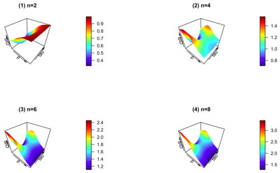
Figure 4.
Plots of the BID when .
From Figure 3, we have the following observations. First, for given , when , the BID is decreasing but greater than 1, except for that of (the BID is less than 1, if 1). Second, when p takes a small value, the BID takes the maximum if takes the boundary value. Third, for the given p and , the BID tends to a greater value when is increasing.
From Figure 4, we have the following observations. First, for , the BID seems to be increasing but lower than 1 when , . Second, for , if takes the non-boundary value, the BID seems to be increasing and then decreasing when ; otherwise, the BID seems to be decreasing. Third, for the given p and , the BID tends to a greater value when is increasing.
To sum up, the discrete beta distribution allows to model bounded data with under-dispersion, equi-dispersion and over-dispersion.
Similar to the statistical-order property of the one-parameter exponential family in [20], Proposition 1 illustrates that it does hold for the distribution.
Proposition 1.
Suppose . If and , then the following conclusions hold and are equivalent:
- (1)
- (2)
- ,
where ,
Proof.
(1) It is easy to see that exhibits the following probability density function
where . Hence,
and
with equality only if and . Hence, Furthermore, by Theorem 4.2 in Wang [21].
(2) Note that if and ,
Hence, , if and , and vice versa. Therefore, The proof is end. □
2.2. Discrete Beta GARCH(1,1) Model with a Nearly Linear Structure
Inspired by Weiß and Jahn [16] and distribution, we give the definition of the ScDBGARCH(1,1) model by
where is the -field generated by , , , and , , or 1 and is the predetermined upper limit of the range.
Note that Proposition 1 presents that the new discrete beta distribution exhibits a statistical-order property, which is similar to the one-parameter exponential family in Davis and Liu [20]. Hence, a natural idea of the stability of the ScDBGARCH model is using the theory of the iterated random function approach [22] to construct the stability properties of the ScDBGARCH model. For this purpose, we first illustrate the stochastic order of the coupling process given in (4), and then account for the moment property of (), which is essential to derive the stability of the proposed model.
Proposition 2.
If satisfies (4), then , if , where “lr” denotes the likelihood ratio.
The result of Proposition 2 can be obtained by Proposition 1, We omit it.
Proposition 3.
For all , if and is the cumulative distribution function of with and , then , where u is a uniform random variable in and .
Proof.
Denote with . Similar to the first item of Proposition 1, if , . Therefore, by Proposition 2, i.e., and . Hence . Similarly, , if . Thus, . The proof is complete. □
In the following, we demonstrate that satisfies the contraction condition by using Lemma A1 in Appendix A, i.e., , , there exist and such that
where and .
Assumption 1.
The parametric space is compact with , , , and .
Theorem 1.
Let satisfy (4). If Assumption 1 and the contraction condition (6) hold, then the following results hold:
- (1)
- If π is a stationary distribution and is independent of , then is geometric-moment contracting with unique stationary distribution π and .
- (2)
- There exists a measurable function such that , i.e., is -measurable, where .
- (3)
- If starts from π, i.e., , then is a stationary time series. Furthermore, is strictly stationary and ergodic.
By Propositions 3 and (6), Theorem 1 can be proved in a similar way in Davis and Liu [20] and Chen et al. [13], and we omit it here.
It is worth mentioning that the incorporated soft-clipping function results in negative auto-regression, besides the positive auto-regression and over-dispersion. Unfortunately, because of the complexity of the discrete beta distribution, we have the closed forms of the auto-regressive coefficient. To get an idea about the abilities of the ScDBGARCH(1,1) model with for explaining different autocorrelation structures, we present some ACF(2)-ACF(1) plots for the ScDBGARCH(1,1) model in Figure 5 and Figure 6. To be precise, for given and or 1, sample size and , we let and with , varying from to with an increment of 0.1, and we compute the values of ACF(1), ACF(2) and plot them against each other.
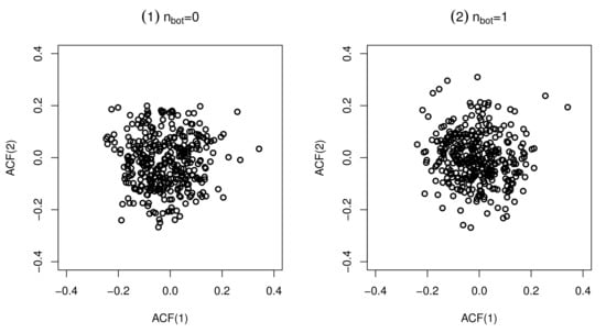
Figure 5.
Plots of attainable pairs of ACF(2) against ACF(1) for with c = 0.01.
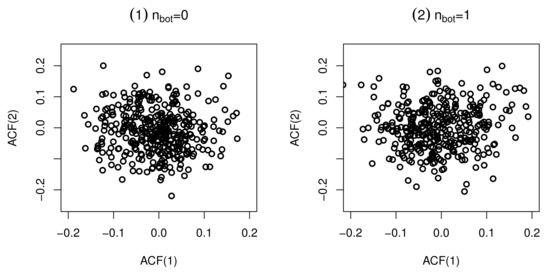
Figure 6.
Plots of attainable pairs of ACF(2) against ACF(1) for with c = 0.01.
From Figure 5 and Figure 6, both negative ACF and non-negative ACF are allowed by the novel ScDBGARCH model, while negative ACF is rejected by the binomial GARCH-type models [10,12], i.e., the novel ScDBGARCH model is much more flexible than the classical binomial GARCH models with respect to the auto-regressive structure.
To be honest, the merit of the model ScDBGARCH goes beyond allowing negative auto-regression, and also allowing under-dispersion. To account for the dispersion, we present the plots of the BID (in Figure 7 and Figure 8) for the ScDBGARCH(1,1) model, for given or 2 and or 1, sample size and when is varying from to with an increment 0.1, and .
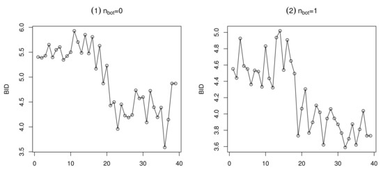
Figure 7.
Plots of BID for with .
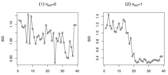
Figure 8.
Plots of BID for with .
From Figure 7 and Figure 8, under-dispersion (besides over-dispersion) is allowed, especially for the ScDBGARCH model with a smaller . Hence, the ScDBGARCH model provides an available way to analyze bounded integer-valued time series counts.
Remark 1.
Similar to the BGARCH(1,1) model [11] and the BBGARCH(1,1) model [13], we can define the following two models:
- Soft-clipping beta-binomial GARCH(1,1) model withwhere , , , and .Obviously, this model, given in (7), is an example of the BBGARCH(1,1) model in [13]. For convenience, we recall it as the ScBBGARCH(1,1) model.
- Soft-clipping binomial GARCH(1,1) model [16] withwhere , , , and .Obviously, this model, given in (8), can be regarded as a further generation of the BARCH-type model; see [10,11,12]. For convenience, we recall it as the ScBGARCH(1,1) model.
3. Parameter Estimation
In this section, we use the conditional maximum likelihood method to estimate the parameters involved in the ScDBGARCH(1,1) model and study their asymptotic behavior. Let . Denote and as the upper and lower ranges, and represents the size of the sample. is a realization of , which can be obtained by the following steps: First, we let and set a pre-run = 500, then generate , where is obtained by (4) and is generated by using function in the ddb package; see Turner [19] for more details. Second, we use as a new initial value of and rewrite it as , then generate .
By (5), the conditional log-likelihood function of (4) can be written as
where , , , , and . Then the CML estimator is obtained by maximizing (9).
Note that in (9) is a constant for a given sample. Hence, the conditional log-likelihood function given in (9) can be simplified and denoted as
and can be obtained by maximizing (10), i.e., is a solution of the score equation
where , , ,
with and .
Furthermore, the Hessian matrix (denoted as ) for model (4) is obtained by further differentiation of the score equation, i.e., with equaling to
where , , , and
with and .
Lemma 1.
Denote . For all , if and only if and , where , , , , or 1 and is considered a known quantity.
Proof.
Note that is continuously differentiable; hence,
Because is strictly increasing in terms of or , so does for
Hence, if and only if and .
To sum up, if and only if and , . □
Assumption 2.
If there exists a such that , a.s., then where is the probability measure under the true parameter and
Assumption 2 establishes the identification of the ScDBGARCH(1,1) model based on Lemma 1.
Theorem 2.
Let be a stationary and ergodic sequence with a finite range and its conditional mean process satisfy (4), the contraction condition (6). If Assumptions 1 and 2 hold, then, as , we obtain the following results:
- (1)
- There exists an estimator such that ;
- (2)
- ,
where and
The proof of Theorem 2 is similar to Theorem 4 in Chen et al. [12]. We omit it.
4. Real Data Example
In this section, we reconsider the number of districts with new cases of measles infection per week in the year 2016–2017 reported in of Germany’s districts. The dataset is taken from the “SurvStat” data (https://survstat.rki.de/Content/Query/Main.aspx) (accessed on 10 December 2022), which have been reported to the Robert Koch Institute by local and state health departments. See Figure 1 for its sample path.
By communication, the sample mean and variances are 4.3173 and 8.3546, respectively. The ACF and PACF plots are given in Figure 9, respectively.
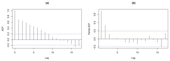
Figure 9.
Measles infection’s counts: (a) ACF, (b) PACF.
Besides the ScDBGARCH(1,1) model, the ScBBGARCH(1,1) model given in (7) and the ScBGARCH(1,1) model given in (8) with , we also choose the following compared models:
- BARCH(p) model [10] with
- logit-BARCH(p) model [12] with
- score-BARCH(1) model [12] with
- BGARCH(1,1) model [11] with
- logit-BBGARCH(1,1) model [13] with and its mean process satisfying .
In the following, we use the above models to fit the measles infection’s data by the CML method and compare their estimated standard error (SE), −log-likelihood (−log-lik), AIC and BIC, where SE is computed by Theorem 2 and . The CML estimates and approximated standard errors of parameters (including the fitted values of −log-lik, AIC and BIC) are summarized in Table 1.

Table 1.
Estimates and SEs in parentheses for the measles infection counts.
From Table 1, we have the following observations. For the BARCH-type models, the BARCH(2) model with a linear transformation takes the smallest −log-lik, AIC and BIC. For the GARCH-type models, the ScDBGARCH(1,1) model takes the smallest −log-lik, AIC and BIC, followed by the ScBGARCH(1,1) model, which may be attributed to the merits of the soft-clipping function.For all compared models, the ScDBGARCH(1,1) model takes the smallest −log-lik, AIC and BIC. Hence, the ScDBGARCH(1,1) model is more suitable for the measles data.
To further check the adequacy of the ScDBGARCH(1,1) model, we analyze its Pearson residuals, which are defined by with and As discussed in Weiß [23], “for an adequate model, its fitted standardized Pearson residuals are expected to be uncorrelated with a mean about 0 and a variance about 1”.
First, we calculate that the mean and variance of the Pearson residuals of the ScDBGARCH(1,1) model are and , which implies that the ScDBGARCH(1,1) model demonstrates adequacy. Second, we give its residual analysis in Figure 10, which also shows that this model does rather well.
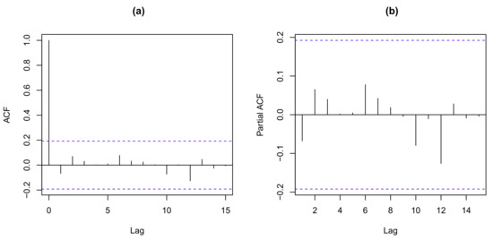
Figure 10.
Pearson residual analysis: (a) ACF, (b) PACF.
Third, we consider the fitted values of the Ljung–Box test based on lags k = 3, 5, 7, 9, 11, 13, and 15, including their p-values and their critical values () with 0.05 confidence, and summarize them in Table 2.

Table 2.
Values of the Ljung–Box test for the measles data.
Table 2 shows that all of the Ljung–Box statistics are less than the corresponding critical values, and the p-values are much greater than the significant level 0.05. Hence, both of them further illustrate the availability of the ScDBGARCH(1,1) model in analyzing the measles data. To sum up, the ScDBGARCH(1,1) model shows better performance in analyzing the measles data.
5. Concluding and Discussion
This paper considers a new and flexible soft-clipping discrete beta GARCH(1,1) model, which not only allows positive correlation, but also negative correlation, as well as under-dispersion, equi-dispersion and over-dispersion. We discuss some properties of the new model, the CML estimate of the parameters involved in the novel model, and the large-sample property of the CML estimate. The applicability and superior of the ScDBGARCH model are illustrated by a real data example.
Like linear binomial ARCH/GARCH-type models [10,11], logit binomial ARCH-type models [12] or beta-binomial GARCH-type models [13], the ScDBGARCH model is applicable to analyze stationary non-negative data with a finite range and will be invalid for data with some time trends. Two natural methods arise, and both of them deserve a detailed analysis in a future project.
One popular method is incorporated into the covariate processes when constructing a new model. Similar to the logit-BBGARCHX model [24] and the PARX model [25], one can establish a model with covariates, taking the ScDBGARCH(1,1) model as an example:
where is a predetermined upper limit of the range, or 1 is a predetermined lower limit of the range, is a d-dimensional exogenous covariate vector, is the -field generated by , , is the additional parameter vector involved in , and is the parameter vector with , and . When discussing the statistical property, an essential and unavoidable point is the specific form of . See Chen and Khamthong [26] for Markov-switching cases.
Specially, if the considered data have a periodic trend, one can consider a s-periodically distributed sequence and its mean process satisfying (4), i.e., the s-periodicity of is understood in the sense that for all , where denotes equality in distribution. To highlight the periodicity, one can consider the model by letting , , and
where , and . See Aknouche et al. [27] for a general periodic mixed Poisson autoregression.
The other popular method is to remove the time trend by using the difference method, but having a negative value emerge (besides non-negative bounded data), i.e., -valued bounded data emerge. As far as we know, existing GARCH-type models are constructed by random rounding operators (see Liu and Yuan [28]), some -valued discrete distributions (see Alomani et al. [29], Carallo et al. [30], Cui et al. [31]), difference of two independent non-negative INGARCH models (see Gonçalves and Mendes-Lopes [32]) and non-negative INGARCH models multiplying by some special -valued discrete random variables (see Xu and Zhu [33]). However, they focus on -valued data with infinite range and cannot apply to bounded data. Hence, a future project in term of the -valued bounded data deserves to be considered.
In addition, as discussed in Chen et al. [6], the Conway–Maxwell–Poisson–binomial AR model shows better performance in analyzing bounded time series counts with under-dispersion, equi-dispersion and over-dispersion. A class of the Conway–Maxwell–Poisson–binomial GARCH model deserves to be considered to analyze volatility for integer-valued time series with a finite range. Similar to Bulla et al. [34] and Chen et al. [35], a signed Conway–Maxwell–Poisson–binomial (SCMPB) thinning operator and a bivariate INAR model based on the SCMPB thinning operator also deserve to be considered to analyze bivariate dependent time series with finite ranges.
Funding
Chen’s work is funded by Natural Science Foundation of Henan Province (No. 222300420127) and Postdoctoral research in Henan Province (No. 202103051).
Data Availability Statement
The number of districts with new cases of measles infection per week in the year 2016–2017 reported in Germany’s districts is taken from the “SurvStat” (https://survstat.rki.de/Content/Query/Main.aspx) on 12 December 2019.
Acknowledgments
The author thanks the Editor-in-Chief and the anonymous referees for the valuable comments and suggestions that resulted in a substantial improvement of this paper. We acknowledge the constructive suggestions from Fukang Zhu of Jilin University on the work.
Conflicts of Interest
The author declares no conflict of interest.
Abbreviations
The following abbreviations are used in this manuscript:
| absolute of x, ; | |
| lr | likelihood ratio; |
| stochastic small; | |
| equality in distribution. | |
| almost surely convergence; | |
| convergence in distribution. |
Appendix A. Auxiliary Results
Lemma A1.
Let Then,
- (1)
- and
- (2)
- and ,
- (3)
- and ;
- (4)
- and .
Proof.
(1) Because is a continuously differentiable function in , exists and
and
by Lemma 4 in [12].
(2) By using the mean value theorem, there exists at least one point such that
where . Hence, and
(3) According to item (1), is a continuously differentiable function in , thus exists and . Furthermore,
by .
(4) By (3), is a continuously differentiable function in , and thus, exists and
Furthermore, by using Lemma 4 in [12], we obtain
The proof is complete. □
Lemma A2.
Let with and . If , then
- (1).
- (2).
- (3).
- where and with .
Proof.
By (2), we compute that
where and . Hence,
Hence, the binomial index of dispersion (BID) of X satisfies
The proof is complete. □
References
- McKenzie, E. Some simple models for discrete variate time series. J. Am. Water Resour. Bull. 1985, 21, 645–650. [Google Scholar] [CrossRef]
- Weiß, C.H.; Testik, M.C. On the Phase I analysis for monitoring time-dependent count processes. IIE Trans. 2015, 47, 294–306. [Google Scholar] [CrossRef]
- Möller, T.A.; Weiß, C.H.; Kim, H.Y.; Sirchenko, A. Modeling zero inflation in count data time series with bounded support. Methodol. Comput. Appl. Probab. 2018, 20, 589–609. [Google Scholar] [CrossRef]
- Chen, H.; Li, Q.; Zhu, F. Binomial AR(1) processes with innovational outliers. Commun. Stat. Theory Methods 2021, 50, 446–472. [Google Scholar] [CrossRef]
- Kang, Y.; Wang, D.; Yang, K. Extended binomial AR(1) processes with generalized binomial thinning operator. Commun. Stat. Theory Methods 2020, 49, 3498–3520. [Google Scholar] [CrossRef]
- Chen, H.; Zhang, J.; Liu, X. A Conway-Maxwell-Poisson-Binomial AR(1) model for bounded time series data. Entropy 2023, 25, 126. [Google Scholar] [CrossRef]
- Shmueli, G.; Minka, T.P.; Kadane, J.B.; Borle, S.; Boatwright, P. A useful distribution for fitting discrete data: Revival of the Conway-Maxwell-Poisson distribution. Appl. Stat. 2005, 54, 127–142. [Google Scholar] [CrossRef]
- Zhang, R.; Wang, D.; Li, C. Flexible binomial AR(1) processes using copulas. J. Stat. Plan. Inference 2022, 219, 306–332. [Google Scholar] [CrossRef]
- Weiß, C.H.; Pollett, P.K. Binomial autoregressive processes with density-dependent thinning. J. Time Ser. Anal. 2014, 35, 115–132. [Google Scholar] [CrossRef]
- Ristić, M.M.; Weiß, C.H.; Janjić, A.D. A binomial integer-valued ARCH model. Int. J. Biostat. 2016, 12, 20150051. [Google Scholar] [CrossRef]
- Lee, Y.; Lee, S. CUSUM test for general nonlinear integer–valued GARCH models: Comparison study. Ann. Inst. Stat. Math. 2019, 71, 1033–1057. [Google Scholar] [CrossRef]
- Chen, H.; Li, Q.; Zhu, F. Two classes of dynamic binomial integer-valued ARCH models. Braz. J. Probab. Stat. 2020, 34, 685–711. [Google Scholar] [CrossRef]
- Chen, H.; Li, Q.; Zhu, F. A new class of integer-valued GARCH models for time series of bounded counts with extra-binomial variation. AStA Adv. Stat. Anal. 2022, 106, 243–270. [Google Scholar] [CrossRef]
- Liu, M.; Zhu, F.; Zhu, K. Modeling normalcy-dominant ordinal time series: An application to air quality level. J. Time Ser. Anal. 2022, 43, 460–478. [Google Scholar] [CrossRef]
- Liu, M.; Li, Q.; Zhu, F. Modeling air quality level with a flexible categorical autoregression. Stoch. Environ. Res. Risk Assess. 36, 2835–2845. [CrossRef]
- Weiß, C.H.; Jahn, M. Soft-clipping INGARCH models for time series of bounded Counts. Stat. Model. 2022. forthcoming. [Google Scholar] [CrossRef]
- Weiß, C.H.; Zhu, F.; Hoshiyar, A. Softplus INGARCH models. Stat. Sin. 2022, 32, 1099–1120. [Google Scholar] [CrossRef]
- Klimek, M.D.; Perelstein, M. Neural network-based approach to phase space integration. SciPost Phys. 2020, 9, 053. [Google Scholar] [CrossRef]
- Turner, R. A new versatile discrete distribution. R J. 2021, 13, 485–506. [Google Scholar] [CrossRef]
- Davis, R.A.; Liu, H. Theory and inference for a class of observation-driven models with application to time series of counts. Stat. Sin. 2016, 26, 1673–1707. [Google Scholar]
- Wang, Z. One mixed negative binomial distribution with application. J. Stat. Plan. Inference 2011, 141, 1153–1160. [Google Scholar] [CrossRef]
- Wu, W.; Shao, X. Limit theorems for iterated random functions. J. Appl. Probab. 2004, 41, 425–436. [Google Scholar] [CrossRef]
- Weiß, C.H. An Introduction to Discrete-Valued Time Series; John Wiley & Sons: Chichester, UK, 2018. [Google Scholar]
- Chen, H.; Li, Q.; Zhu, F. A covariate-driven beta-binomial integer-valued GARCH model for bounded counts with an application. Metrika 2023. forthcoming. [Google Scholar] [CrossRef]
- Agosto, A.; Cavaliere, G.; Kristensen, D.; Rahbek, A. Modeling corporate defaults: Poisson autoregressions with exogenous covariates (PARX). J. Empir. Financ. 2016, 38, 640–663. [Google Scholar] [CrossRef]
- Chen, C.W.S.; Khamthong, K. Bayesian modelling of nonlinear negative binomial integer-valued GARCHX models. Stat. Model. 2020, 20, 537–561. [Google Scholar] [CrossRef]
- Aknouche, A.; Bentarzi, W.; Demouche, N. On periodic ergodicity of a general periodic mixed Poisson autoregression. Stat. Probab. Lett. 2018, 134, 15–21. [Google Scholar] [CrossRef]
- Liu, T.; Yuan, X. Random rounded integer-valued autoregressive conditional heteroskedastic process. Stat. Pap. 2013, 54, 645–683. [Google Scholar] [CrossRef]
- Alomani, G.A.; Alzaid, A.A.; Omair, M.A. A Skellam INGARCH model. Braz. J. Probab. Stat. 2018, 32, 200–214. [Google Scholar] [CrossRef]
- Carallo, G.; Casarin, R.; Robert, C.P. Generalized Poisson difference autoregressive processes. arXiv 2020, arXiv:2002.04470. [Google Scholar]
- Cui, Y.; Li, Q.; Zhu, F. Flexible bivariate Poisson integer-valued GARCH model. Ann. Inst. Stat. Math. 2020, 72, 1449–1477. [Google Scholar] [CrossRef]
- Gonçalves, E.; Mendes-Lopes, N. Signed compound Poisson integer-valued GARCH processes. Commun. Stat. Theory Methods 2020, 49, 5468–5492. [Google Scholar] [CrossRef]
- Xu, Y.; Zhu, F. A new GJR-GARCH model for Z-valued time series. J. Time Ser. Anal. 2022, 43, 490–500. [Google Scholar] [CrossRef]
- Bulla, J.; Chesneau, C.; Kachour, M. A bivariate first-order signed integer-valued autoregressive process. Commun. Stat. Theory Methods 2017, 46, 6590–6604. [Google Scholar] [CrossRef]
- Chen, H.; Zhu, F.; Liu, X. Two-step conditional least squares estimation for the bivariate Z-valued INAR(1) model with bivariate Skellam innovations. Commun. Stat. Theory Methods 2023. forthcoming. [Google Scholar] [CrossRef]
Disclaimer/Publisher’s Note: The statements, opinions and data contained in all publications are solely those of the individual author(s) and contributor(s) and not of MDPI and/or the editor(s). MDPI and/or the editor(s) disclaim responsibility for any injury to people or property resulting from any ideas, methods, instructions or products referred to in the content. |
© 2023 by the author. Licensee MDPI, Basel, Switzerland. This article is an open access article distributed under the terms and conditions of the Creative Commons Attribution (CC BY) license (https://creativecommons.org/licenses/by/4.0/).