The Lookup Table Regression Model for Histogram-Valued Symbolic Data
Abstract
1. Introduction
2. Representation of Objects by Quantile Vectors and Bin Rectangles
2.1. Histogram-Valued Feature
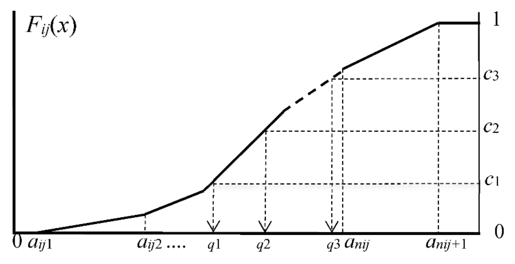
2.2. Representation of Histograms by Common Number of Quantiles
- (1)
- We choose common number m of quantiles.
- (2)
- Let c1, c2, ..., cm−1 be preselected cut points dividing the range of the distribution function Fij(x) into continuous intervals, i.e., bins, with preselected probabilities associated with m cut points.
- (3)
- For the given cut points c1, c2, ..., cm−1, we have the corresponding quantiles by solving the following equations:
2.3. Quantile Vectors and Bin-Rectangles
3. Monotone Blocks Segmentation (MBS) and Lookup Table Regression Model (LTRM)
- Our Fats and Oils data is composed of six plant oils and only two animal fats. By increasing the number of sample objects, we may obtain more accurate Lookup Table.
- On the other hand, increasing the number of sample objects may complicate the covariate relations between the response variable and explanatory variables. For example, if we separate the plant oils and animal fats, we may have better Lookup Tables for respective categories.
4. Multi-Lookup Table Regression Model (M-LTRM)
4.1. Illustration by Oval Data
4.2. Hierarchical Conceptual Clustering
- (1)
- 0 ≤ C(ωi, ωl) ≤ 1
- (2)
- C(ωi, ωi), C(ωl, ωl) ≤ C(ωi, ωl)
- (3)
- C(ωi, ωl) = C(ωl, ωi)
- (4)
- C(ωi, ωr) ≤ C(ωi, ωl) + C(ωl, ωr) may not hold in general.
| Algorithm 1 (Hierarchical Conceptual Clustering (HCC) [16]) |
| Step 1: For each pair of objects ωi and ωl in U, evaluate the compactness C(ωi, ωl) and find the pair ωq and ωr that minimizes the compactness. Step 2: Add the merged concept ωqr = {ωq, ωr} to U and delete ωq and ωr from U. The merged concept ωqr is again described using p histograms as Eqr = Eqr1 × Eqr2 × ··· × Eqrp by the Cartesian join operation defined in [16] under the assumption of m quantiles and the equal bin probabilities. Step 3: Repeat Step 1 and Step 2 until U includes only one concept, i.e., the whole concept. |
- The MBS is able to detect a covariate relation between the response variable and explanation variable(s), if the covariate relation has a monotone structure. In other words, the MBS has a feature selection capability when the target covariate relation has a monotone structure.
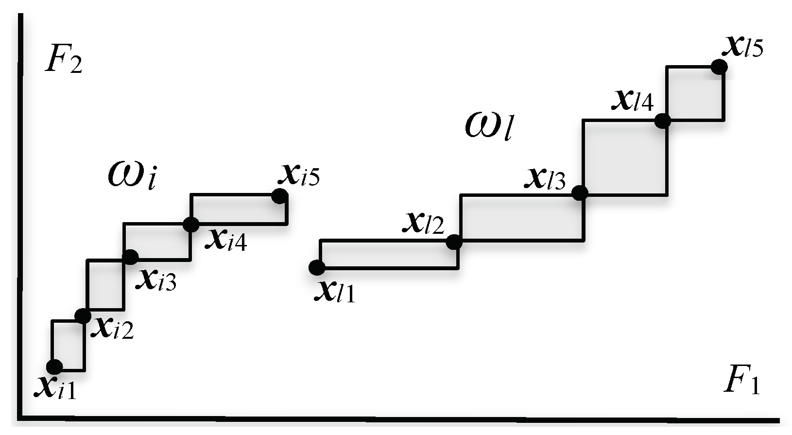
- On the other hand, the unsupervised feature selection method using hierarchical conceptual clustering in [16] can detect “geometrically thin structures” embedded in the given histogram-valued data. The covariation of F1 and F2 is found by evaluating the compactness for each of five features in each step of clustering [16]. Therefore, the compactness plays also the role of feature effectiveness criterion.
4.3. M-LTRM for the Hardwood Data
- F1: Annual Temperature (ANNT) (°C);
- F2: January Temperature (JANT) (°C);
- F3: July Temperature (JULT) (°C);
- F4: Annual Precipitation (ANNP) (mm);
- F5: January Precipitation (JANP) (mm);
- F6: July Precipitation (JULP) (mm);
- F7: Growing Degree Days on 5 °C base ×1000 (GDC5);
- F8: Moisture Index (MITM).
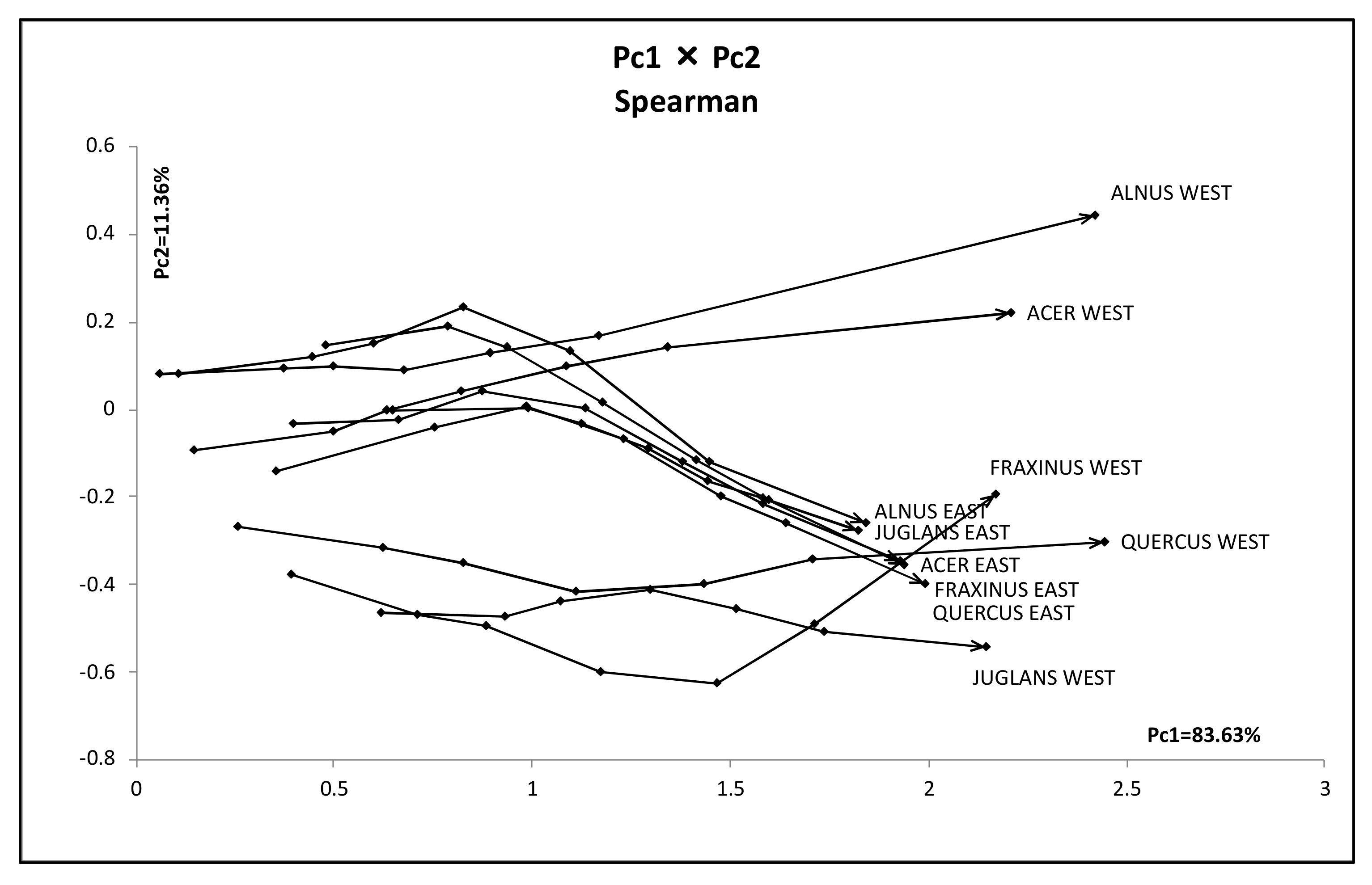
- The first principal component is the size factor and the second is the shape factor, and the sum of their contribution ratios is very high.
- East hardwoods show similar line graphs, and the maximum quantile vectors take mutually near positions.
- West hardwoods are separated into two groups: {ACER WEST and ALNUS WEST} and {FRAXINUS WEST, JUGLANS WEST, and QUERCUS WEST}. The last line segments are very long especially for ACER WEST and ALNUS WEST.
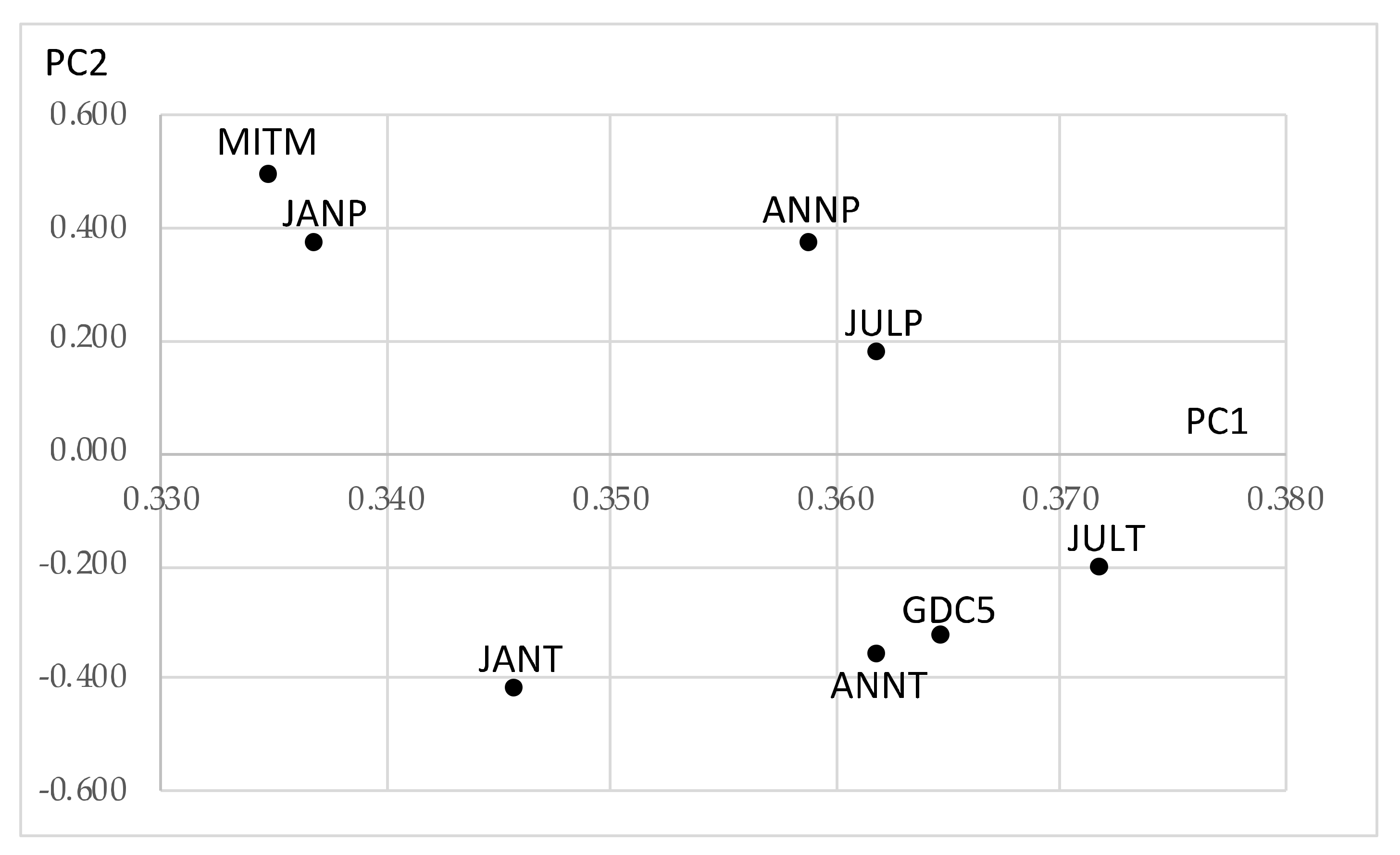
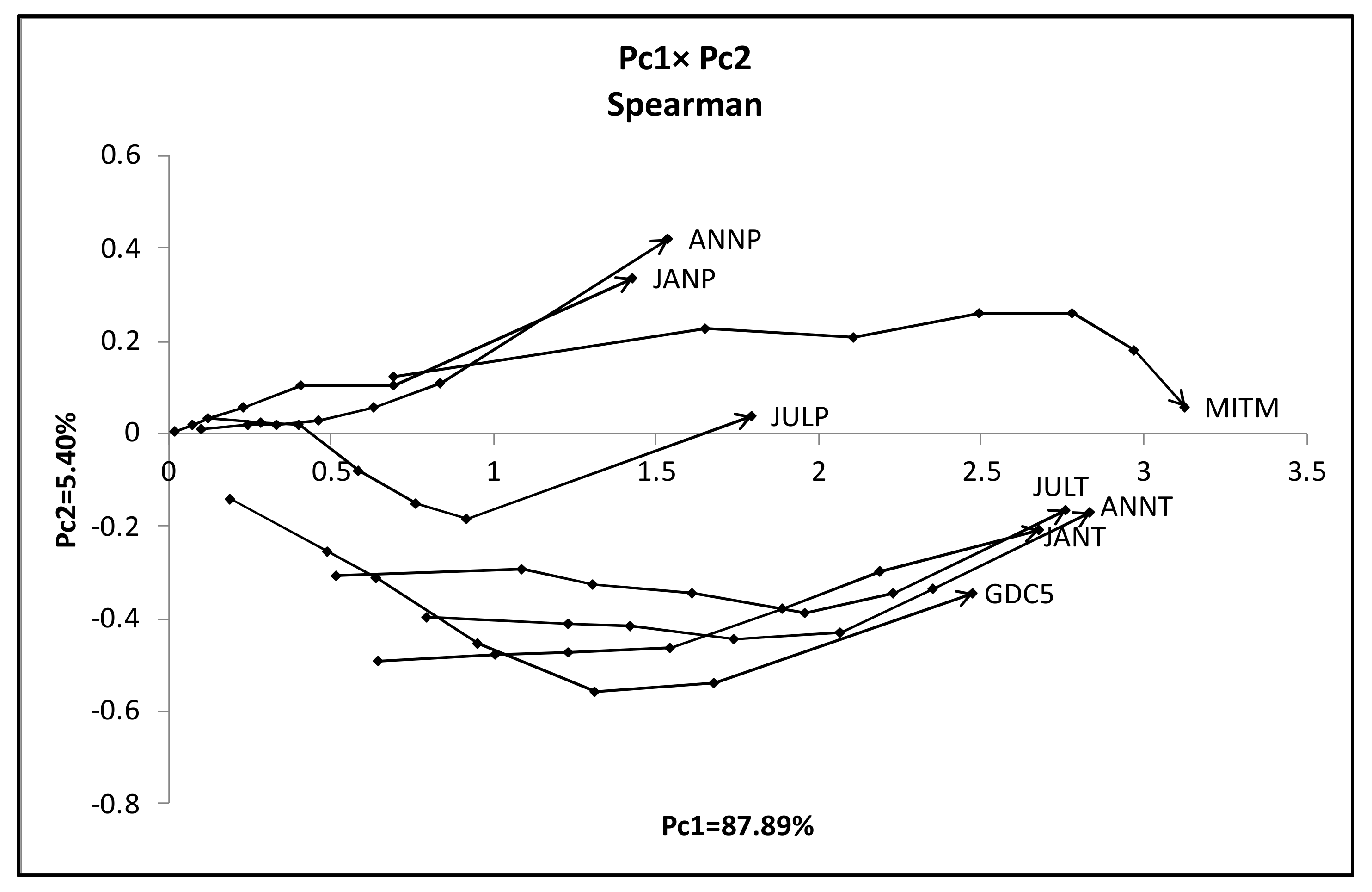
- The first principal component is the size factor and the second is the shape factor, and the sum of their contribution ratios is very high.
- We have two groups {ANNP, JANP, JULP, and MITM} and {ANNT, JANT, JULT, and GDC5}. MITM and GDC5 are very long line graphs compared to other members in each group.
5. Discussion
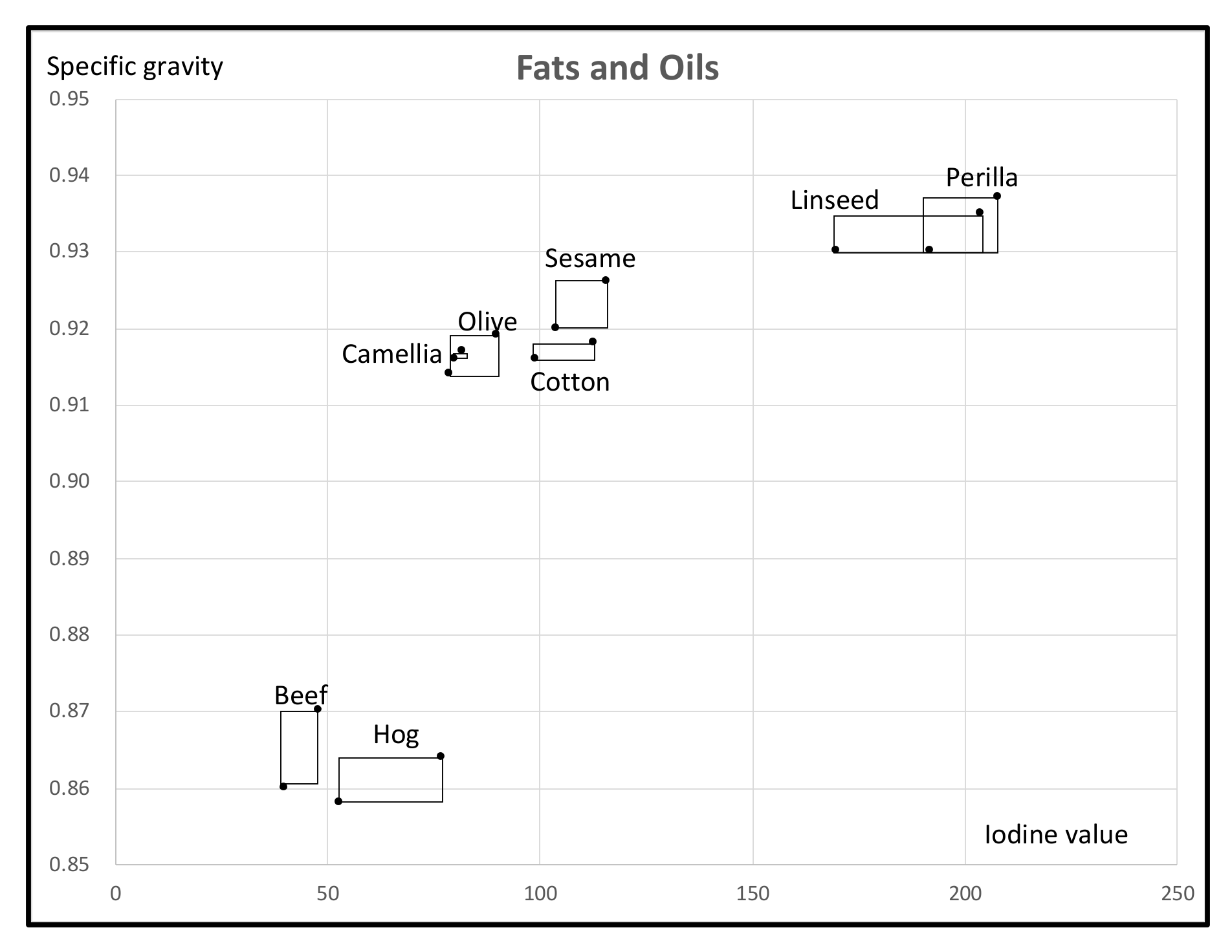
- As a mixed feature-type symbolic data, we used the Fats and Oils data. This data is organized from eight objects, two fats and six plant oils, described by four interval valued features and one multinominal feature. By the quantile method, we transformed to a numerical data table of the size (8 × 2 quantiles) × (5 features). Then, we applied our MBS to this data under the assumption that the response variable is Iodine value. The MBS selected Specific gravity as the most covariate feature to Iodine value, then Freezing point. By using the obtained Lookup Table, we checked the estimation of Iodine value of each given object using Specific gravity and Freezing point. The estimated result is reasonable for the given fats and oils. We also checked our Lookup Table by a set of independent fats and oils. The result by test samples suggests the use of clustering and Multi-Lookup Table Regression Model (M-LTRM) to improve the estimation accuracy.
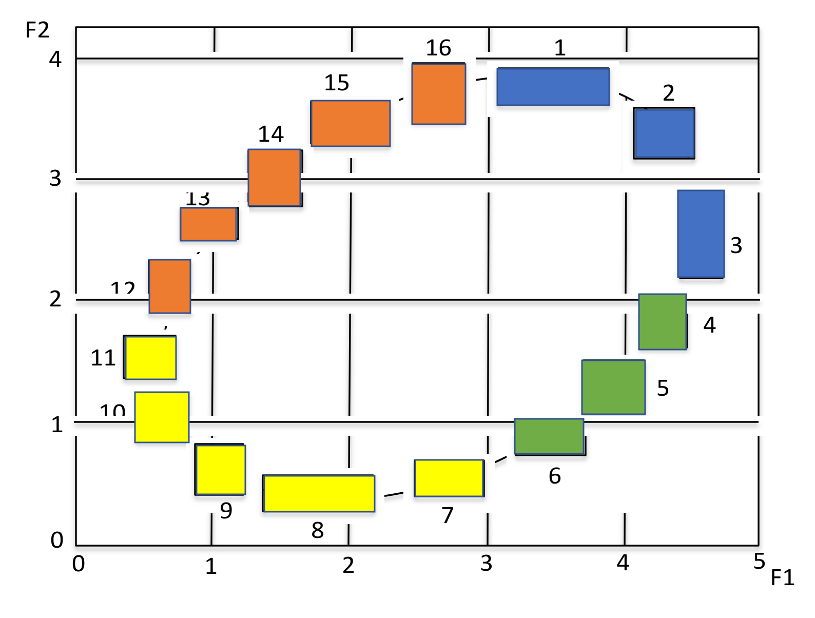
- The MBS works well to generate a meaningful Lookup Table, when the response variable and explanatory variable(s) follow to a monotone structure. Therefore, if the response variable and explanatory variable(s) follow to non-monotonic data structure, we have to divide the given data structure into several monotone substructures. We used the hierarchical conceptual clustering in [16] to the Oval artificial data, and we could obtain four monotone substructures and corresponding Lookup Tables.
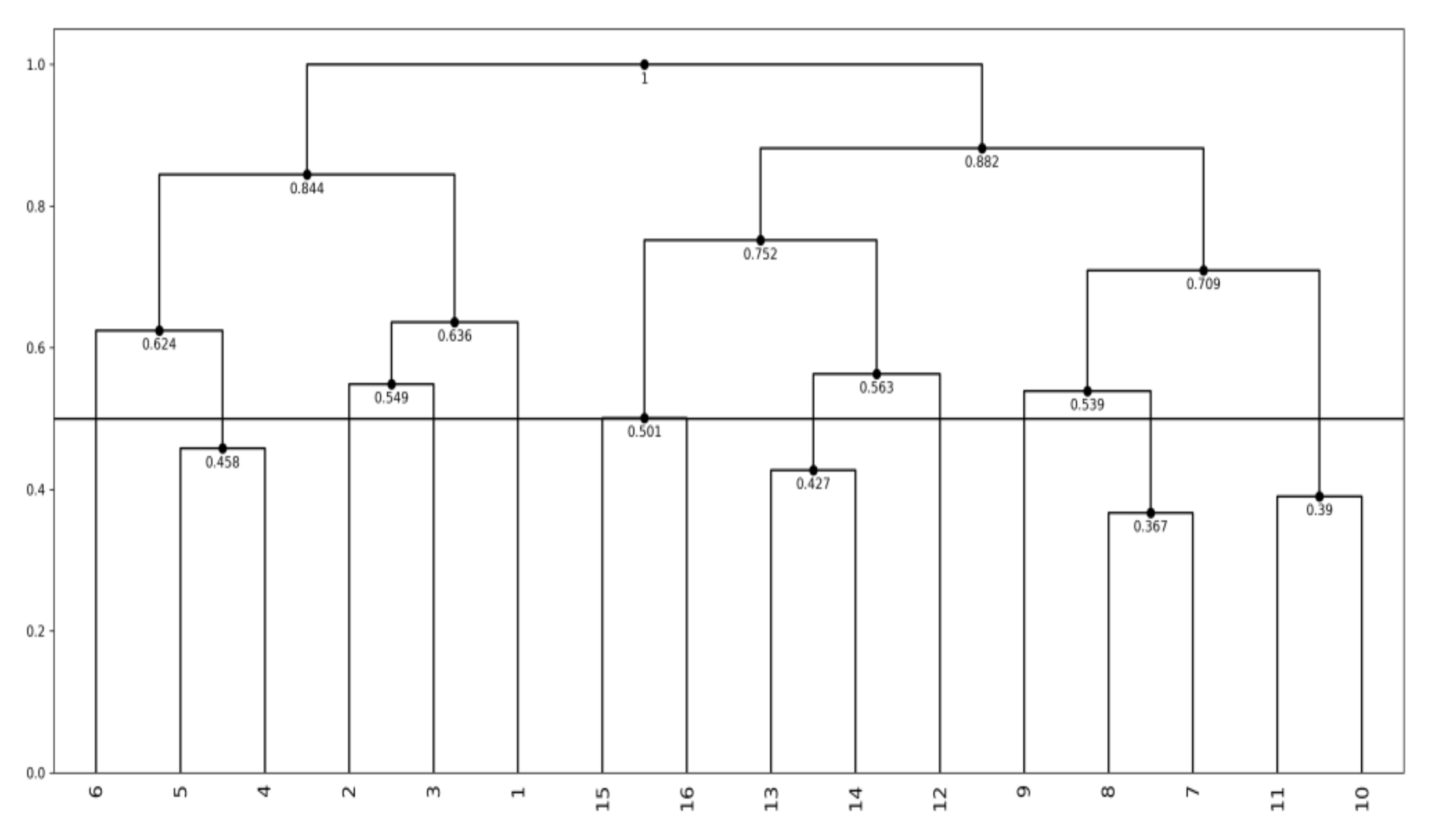
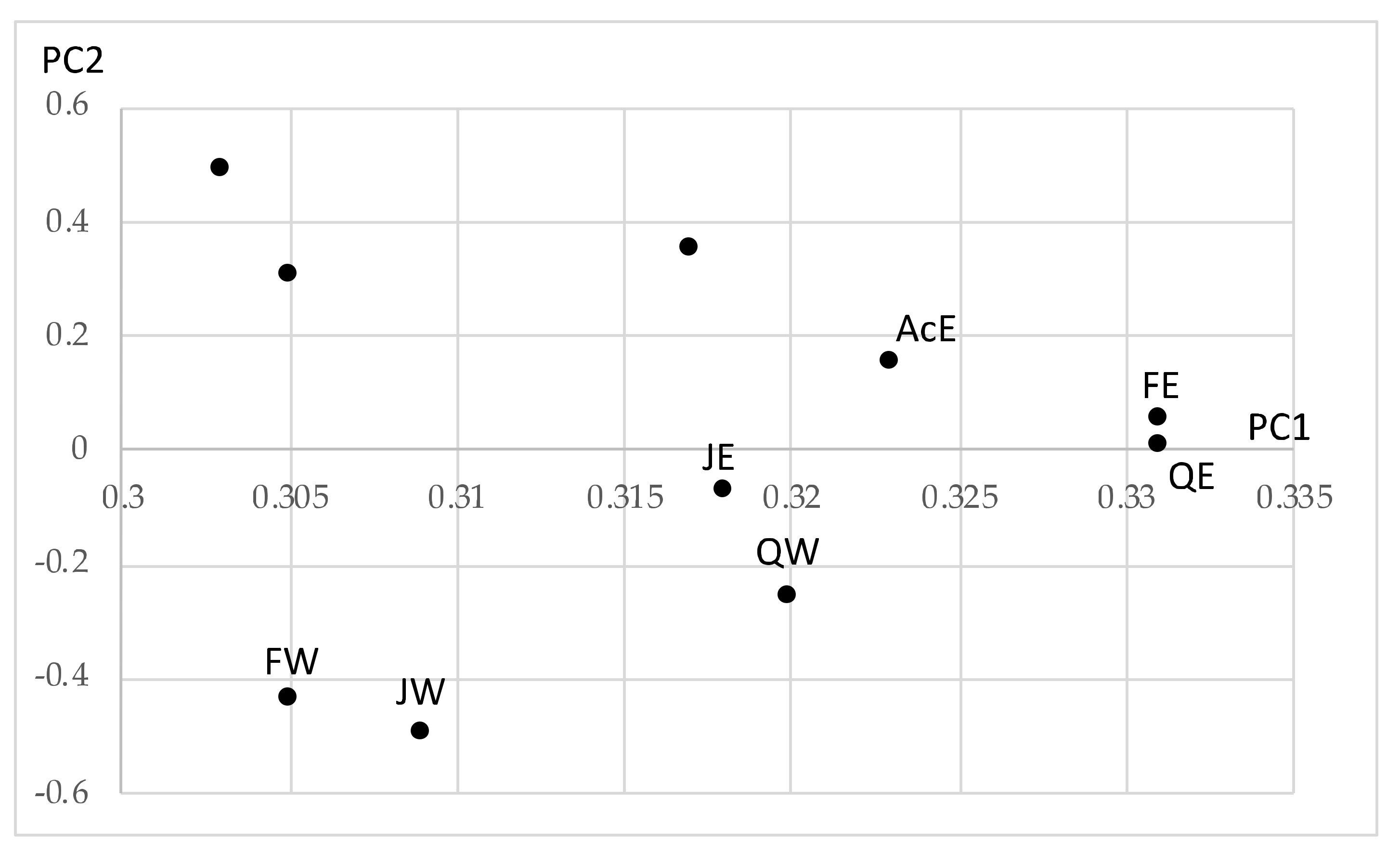
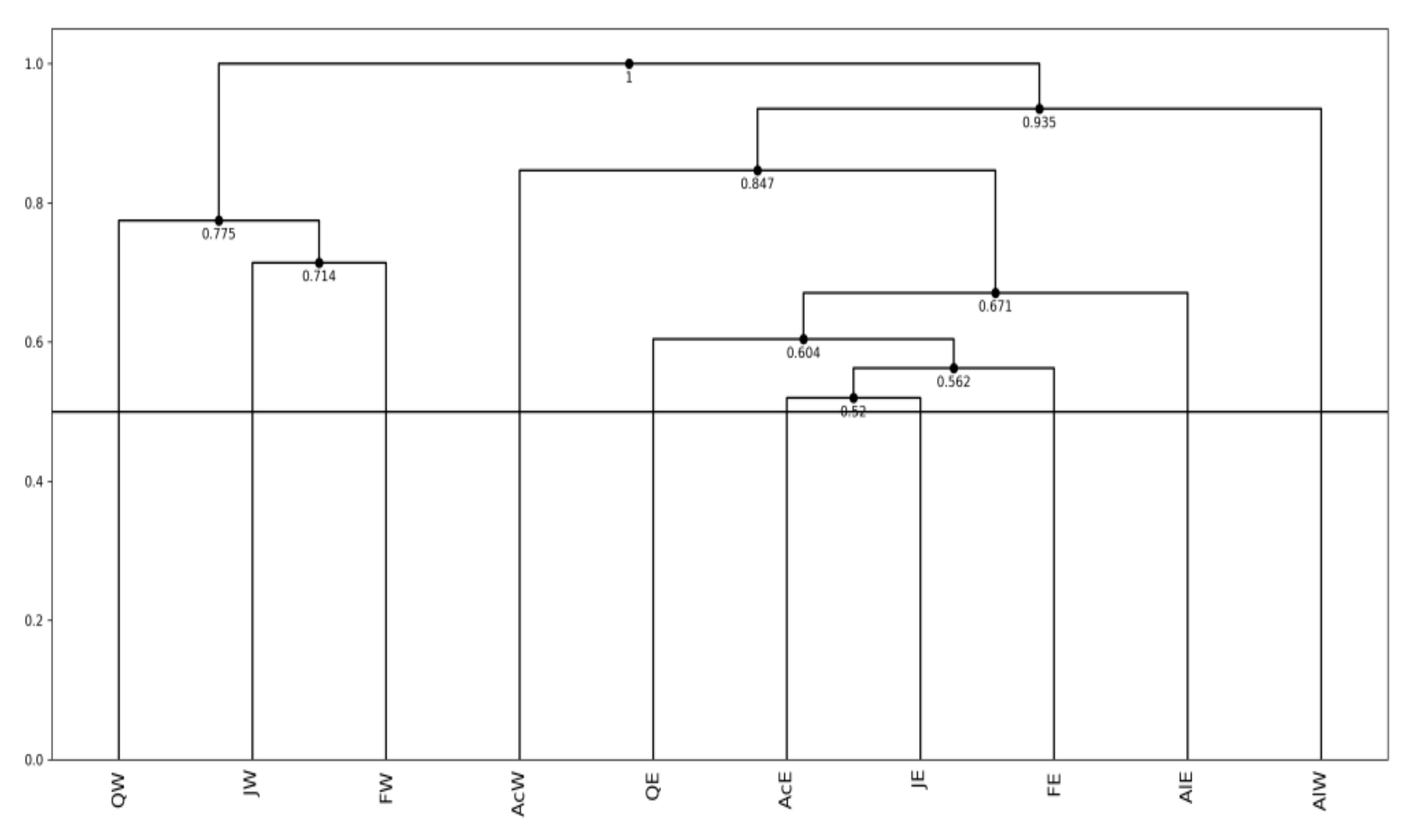
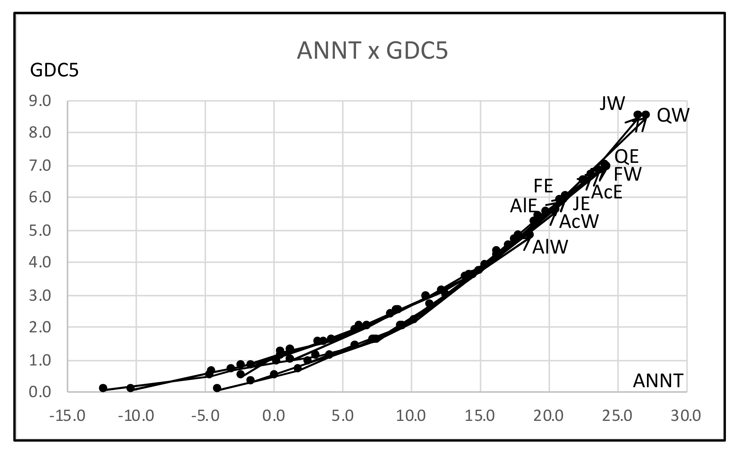
- As a general histogram-valued data, we used the Hardwood data of the size {(10 objects) × (7 quantiles)} × (8 features). We applied the quantile method of Spearman PCA to this data. As a monotone structure, the first factor plane draws three streams C1 = (AcW, AlW), C2 = (AcE, AlE, FE, JE, QE), and C3 = (FW, JW, QW) with a very high contribution ratio. We applied also the Spearman PCA to the dual data of the size {(8 features) × (7 quantiles)} × (10 objects), and we obtained a monotone structure composed of two groups, (ANNP, JANP, JULP, MITM) and (ANNT, JANT, JULT, GDC5) in the first factor plane with a very high contribution ratio. We applied the MBS to the Hardwood data under the assumption that GDC5 is the response variable, and obtained the Lookup Table with explanatory variables: ANNT, JANT, and JULT. Therefore, our MBS has the ability of supervised feature selection.
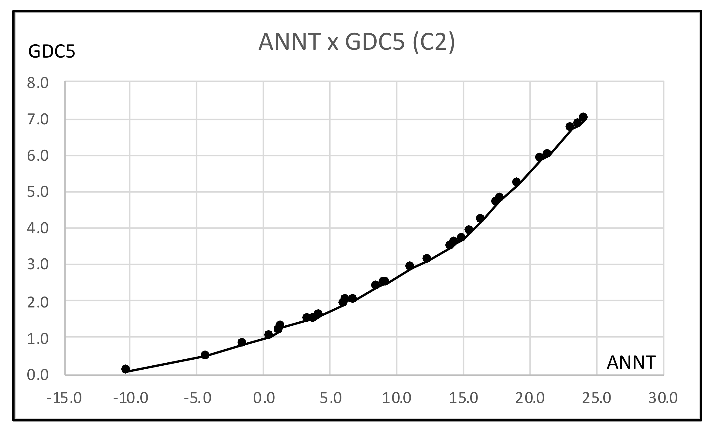
- For a further improvement of the Lookup Table, we applied the hierarchical conceptual clustering to the Hardwood data, and obtained again three clusters: C1, C2, and C3. From the view point of unsupervised feature selection by the hierarchical conceptual clustering, features ANNP then JULP are informative during 1~7 steps of clustering, and JANT is important to separate between clusters (C1, C2) and C3. In fact, the scatter plot of ten hardwoods in the plane ANNP and JANT is very similar to the result of PCA for the Hardwood data. We applied again the MBS to each of clusters C1, C2, and C3, and we obtained three different Lookup Tables. As the result, the Lookup Table for C2 has the highest resolution to estimate GDC5 using ANNT, and it achieves the better estimation result for our test data.
6. Conclusions
Funding
Institutional Review Board Statement
Informed Consent Statement
Data Availability Statement
Acknowledgments
Conflicts of Interest
References
- Bock, H.-H.; Diday, E. Analysis of Symbolic Data; Springer: Berlin/Heidelberg, Germany, 2000. [Google Scholar]
- Billard, L.; Diday, E. Symbolic Data Analysis: Conceptual Statistics and Data Mining; Wiley: Chichester, UK, 2007. [Google Scholar]
- Billard, L.; Diday, E. Regression analysis for interval-valued data. In Data Analysis, Classification and Related Metods. Proceedings of the Conference of the International Federation of Classification Societies (IFCS’00); Springer: Berlin/Heidelberg, Germany, 2000; pp. 347–369. [Google Scholar]
- Diday, E. Thinking by classes in data science: The symbolic data analysis paradigm. WIREs Comput. Stat. 2016, 8, 172–205. [Google Scholar] [CrossRef]
- Verde, R.; Irpino, A. Ordinary least squares for histogram data based on Wasserstein distance. In Proceedings of the COM-STAT’, Paris, France, 22–27 August 2010; Lechevallier, Y., Saporta, G., Eds.; Physica-Verlag: Heidelberg, Germany, 2010; pp. 581–589. [Google Scholar]
- Irpino, A.; Verde, R. Linear regression for numeric symbolic variables: Ordinary least squares approach based on Wasserstein Distance. Adv. Data Anal. Classif. 2015, 9, 81–106. [Google Scholar] [CrossRef]
- Neto, L.; Carvalho, D. Center and range method for fitting a linear regression model for symbolic interval data. Comput. Stat. Data Anal. 2008, 52, 1500–1515. [Google Scholar] [CrossRef]
- Neto, L.; Carvalho, D. Constrained linear regression models for symbolic interval-valued variables. Comput. Stat. Data. Anal. 2010, 54, 333–347. [Google Scholar] [CrossRef]
- Neto, L.; Cordeiro, M.; Carvalho, D. Bivariate symbolic regression models for interval-valued variables. J. Stat. Comput. Simul. 2011, 81, 1727–1744. [Google Scholar] [CrossRef]
- Dias, S.; Brito, P. Linear regression model with Histogram-valued variables. Stat. Anal. Data Min. 2015, 8, 75–113. [Google Scholar] [CrossRef]
- Dias, L.; Brito, P. (Eds.) Analysis of Distributional Data; CRC Press: Boca Raton, FL, USA, 2022. [Google Scholar]
- Ichino, M.; Yaguchi, H. Generalized Minkowski metrics for mixed feature-type data analysis. IEEE Trans. Syst. Man Cybern. 1994, 24, 698–708. [Google Scholar] [CrossRef]
- Ono, Y.; Ichino, M. A new feature selection method based on geometrical thickness. In Proceedings of the KESDA’98, Luxembourg, 27–28 April 1998; Volume 1, pp. 19–38. [Google Scholar]
- Ichino, M. The lookup table regression model for symbolic data. In Proceedings of the Data Sciences Workshop, Paris-Dauphin University, Paris, France, 12–13 November 2015. [Google Scholar]
- Ichino, M. The quantile method of symbolic principal component analysis. Stat. Anal. Data Min. 2011, 4, 184–198. [Google Scholar] [CrossRef]
- Ichino, M.; Umbleja, K.; Yaguchi, H. Unsupervised feature selection for histogram-valued symbolic data using hierarchical conceptual clustering. Stats 2021, 4, 359–384. [Google Scholar] [CrossRef]
- Histogram Data by the U.S. Geological Survey, Climate-Vegetation Atlas of North America. Available online: http://pubs.usgs.gov/pp/p1650-b/ (accessed on 11 November 2010).

| Specific Gravity (g/cm3): F1 | Freezing Point (°C): F2 | Iodine Value: F3 | Saponification Value:F4 | Major Acids: F5 | |
|---|---|---|---|---|---|
| Linseed | [0.930, 0.935] | [−27, −18] | [170, 204] | [118, 196] | L, Ln, O, P, M |
| Perilla | [0.930, 0.937] | [−5, −4] | [192, 208] | [188, 197] | L, Ln, O, P, S |
| Cotton | [0.916, 0.918] | [−6, −1] | [99, 113] | [189, 198] | L, O, P, M, S |
| Sesame | [0.920, 0.926] | [−6, −4] | [104, 116] | [187, 196] | L, O, P, S, A |
| Camellia | [0.916, 0.917] | [−21, −15] | [80, 82] | [189, 193] | L, O |
| Olive | [0.914, 0.919] | [0, 6] | [79, 90] | [190, 199] | L, O, P, S |
| Beef | [0.860, 0.870] | [30, 38] | [40, 48] | [190, 199] | O, P, M, S, C |
| Hog | [0.858,0.864] | [22, 32] | [53, 77] | [190, 202] | L, O, P, M, S, Lu |
| Specific Gravity | Freezing Point | Iodine Value | Saponification Value | Major Acids | |
|---|---|---|---|---|---|
| Linseed 1 | 0.930 | −27 | 170 | 118 | 4 |
| Linseed 2 | 0.935 | −18 | 204 | 196 | 9 |
| Perilla 1 | 0.930 | −5 | 192 | 188 | 4 |
| Perilla 2 | 0.937 | −4 | 208 | 197 | 9 |
| Cotton 1 | 0.916 | −6 | 99 | 189 | 5 |
| Cotton 2 | 0.918 | −1 | 113 | 198 | 9 |
| Sesame 1 | 0.920 | −6 | 104 | 187 | 2 |
| Sesame 2 | 0.926 | −4 | 116 | 193 | 9 |
| Camellia 1 | 0.916 | −21 | 80 | 189 | 8 |
| Camellia 2 | 0.917 | −15 | 82 | 193 | 9 |
| Olive 1 | 0.914 | 0 | 79 | 187 | 6 |
| Olive 2 | 0.919 | 6 | 90 | 196 | 9 |
| Beef 1 | 0.860 | 30 | 40 | 190 | 2 |
| Beef 2 | 0.870 | 38 | 48 | 199 | 9 |
| Hog 1 | 0.858 | 22 | 53 | 190 | 1 |
| Hog 2 | 0.864 | 32 | 77 | 202 | 9 |
| Iodine Value | Specific Gravity | Freezing Point | Saponification Value | Major Acids | |
|---|---|---|---|---|---|
| Beef 1 | 40 | 0.860 | 30 | 190 | 3 |
| Beef 2 | 48 | 0.870 | 38 | 199 | 9 |
| Hog 1 | 53 | 0.858 | 22 | 190 | 1 |
| Hog 2 | 77 | 0.864 | 32 | 202 | 9 |
| Olive 1 | 79 | 0.914 | 0 | 187 | 6 |
| Camellia 1 | 80 | 0.916 | −21 | 189 | 8 |
| Camellia 2 | 82 | 0.917 | −15 | 193 | 9 |
| Olive 2 | 90 | 0.919 | 6 | 196 | 9 |
| Cotton 1 | 99 | 0.916 | −6 | 189 | 5 |
| Sesame 1 | 104 | 0.920 | −6 | 187 | 2 |
| Cotton 2 | 113 | 0.918 | −1 | 198 | 9 |
| Sesame 2 | 116 | 0.926 | −4 | 193 | 9 |
| Linseed 1 | 170 | 0.930 | −27 | 118 | 4 |
| Perilla 1 | 192 | 0.930 | −5 | 188 | 4 |
| Linseed 2 | 204 | 0.935 | −18 | 196 | 9 |
| Perilla 2 | 208 | 0.937 | −4 | 197 | 9 |
| Iodine Value | Specific Gravity | Freezing Point |
|---|---|---|
| [40, 77] | [0.858, 0.870] | [22, 38] |
| [79, 79] | [0.914, 0.914] | |
| [79, 208] | [−27, 6] | |
| [80, 113] | [0.916, 0.920] | |
| [116, 116] | [0.926, 0.926] | |
| [170, 192] | [0.930, 0.930] | |
| [204, 204] | [0.935, 0.935] | |
| [208, 208] | [0.937, 0.937] |
| Fats and Oils | Estimated by | Estimated by | Actual Value |
|---|---|---|---|
| Specific Gravity | Freezing Point | ||
| Linseed | [170, 204] | [79, 208] | [170, 204] |
| Perilla | [170, 208] | [79, 208] | [188, 197] |
| Cotton | [80, 113] | [79, 208] | [99, 113] |
| Sesame | [113, 116] | [79, 208] | [104, 116] |
| Camellia | [80, 113] | [79, 208] | [80, 82] |
| Olive | [79, 113] | [79, 208] | [79, 90] |
| Beef | [40, 77] | [40, 77] | [40, 48] |
| Hog | [40, 77] | [40, 77] | [55, 77] |
| Fats and Oils | Specific Gravity | Freezing Point | Iodine Value |
|---|---|---|---|
| Corn | [0.920, 0.928] | [−18, −10] | [88, 147] |
| Soybeen | [0.922, 0.934] | [−7, −8] | [114, 138] |
| Rice bran | [0.916, 0.922] | [−10, −5] | [92, 115] |
| Horse fat | [0.90, 0.95] | [30, 35] | [65, 95] |
| Sheep tallow | [0.89, 0.90] | [30, 35] | [35, 46] |
| Chiken fat | [0.91, 0.92] | [30, 32] | [76, 80] |
| Fats and Oils | Estimated by | Estimated by | Actual Value |
|---|---|---|---|
| Specific Gravity | Freezing Point | ||
| Corn | [113, 170] | [79, 208] | [88, 147] |
| Soybeen | [113, 204] | [79, 208] | [114, 138] |
| Rice bran | [80, 113] | [79, 208] | [92, 115] |
| Horse fat | [79, 208] | [40, 77] | [65, 95] |
| Sheep tallow | [77, 79] | [40, 77] | [35, 46] |
| Chiken fat | [79, 113] | [40, 77] | [76, 80] |
| F1 | F2 | F3 | F4 | F5 | |
|---|---|---|---|---|---|
| 1 | [0.629, 0.798] | [0.905, 0.986] | [0.000, 0.982] | [0.002, 0.883] | [0.360, 0.380] |
| 2 | [0.854, 0.955] | [0.797, 0.905] | [0.002, 0.421] | [0.573, 1.000] | [0.754, 0.761] |
| 3 | [0.921, 1.000] | [0.527, 0.716] | [0.193, 0.934] | [0.035, 0.477] | [0.406, 0.587] |
| 4 | [0.865, 0.933] | [0.378, 0.500] | [0.452, 0.854] | [0.213, 0.604] | [0.000, 0.074] |
| 5 | [0.775, 0.876] | [0.257, 0.338] | [0.300, 0.614] | [0.425, 0.979] | [0.217, 0.568] |
| 6 | [0.663, 0.764] | [0.135, 0.216] | [0.712, 1.000] | [0.904, 0.968] | [0.103, 0.950] |
| 7 | [0.494, 0.596] | [0.041, 0.122] | [0.293, 0.470] | [0.023, 0.086] | [0.765, 0.902] |
| 8 | [0.225, 0.427] | [0.000, 0.081] | [0.633, 0.872] | [0.000, 0.582] | [0.719, 0.852] |
| 9 | [0.112, 0.213] | [0.041, 0.149] | [0.167, 0.802] | [0.056, 0.129] | [0.124, 0.642] |
| 10 | [0.022, 0.112] | [0.162, 0.270] | [0.026, 0.718] | [0.418, 0.851] | [0.549, 0.853] |
| 11 | [0.000, 0.090] | [0.297, 0.392] | [0.096, 0.759] | [0.438, 0.938] | [0.495, 0.760] |
| 12 | [0.045, 0.112] | [0.446, 0.554] | [0.826, 0.962] | [0.230, 0.755] | [0.104, 0.189] |
| 13 | [0.101, 0.202] | [0.608, 0.676] | [0.367, 0.570] | [0.236, 0.684] | [0.683, 0.930] |
| 14 | [0.213, 0.292] | [0.676, 0.811] | [0.371, 0.381] | [0.086, 0.305] | [0.009, 1.000] |
| 15 | [0.315, 0.438] | [0.811, 0.919] | [0.049, 0.585] | [0.056, 0.891] | [0.528, 0.881] |
| 16 | [0.483, 0.562] | [0.878, 1.000] | [0.402, 0.609] | [0.150, 0.769] | [0.207, 0.732] |
| F1 | F2 | F3 | F4 | F5 | |
|---|---|---|---|---|---|
| 111 | 0 | 0.297 | 0.096 | 0.438 | 0.495 |
| 101 | 0.022 | 0.162 | 0.026 | 0.418 | 0.549 |
| 121 | 0.045 | 0.446 | 0.826 | 0.23 | 0.104 |
| 112 | 0.09 | 0.392 | 0.759 | 0.938 | 0.76 |
| 131 | 0.101 | 0.608 | 0.367 | 0.236 | 0.683 |
| 91 | 0.112 | 0.041 | 0.167 | 0.056 | 0.124 |
| 102 | 0.112 | 0.27 | 0.718 | 0.851 | 0.853 |
| 122 | 0.112 | 0.554 | 0.962 | 0.755 | 0.189 |
| 132 | 0.202 | 0.676 | 0.57 | 0.684 | 0.93 |
| 92 | 0.213 | 0.149 | 0.802 | 0.129 | 0.642 |
| 141 | 0.213 | 0.676 | 0.371 | 0.086 | 0.009 |
| 81 | 0.225 | 0 | 0.633 | 0 | 0.719 |
| 142 | 0.292 | 0.811 | 0.381 | 0.305 | 1 |
| 151 | 0.315 | 0.811 | 0.049 | 0.056 | 0.528 |
| 82 | 0.427 | 0.081 | 0.872 | 0.582 | 0.852 |
| 152 | 0.438 | 0.919 | 0.585 | 0.891 | 0.881 |
| 161 | 0.483 | 0.878 | 0.402 | 0.15 | 0.207 |
| 71 | 0.494 | 0.041 | 0.293 | 0.023 | 0.765 |
| 162 | 0.562 | 1 | 0.609 | 0.769 | 0.732 |
| 72 | 0.596 | 0.122 | 0.47 | 0.086 | 0.902 |
| 11 | 0.629 | 0.905 | 0 | 0.002 | 0.36 |
| 61 | 0.663 | 0.135 | 0.712 | 0.904 | 0.103 |
| 62 | 0.764 | 0.216 | 1 | 0.968 | 0.95 |
| 51 | 0.775 | 0.257 | 0.3 | 0.425 | 0.217 |
| 12 | 0.798 | 0.986 | 0.982 | 0.883 | 0.38 |
| 21 | 0.854 | 0.797 | 0.002 | 0.673 | 0.754 |
| 41 | 0.865 | 0.378 | 0.452 | 0.213 | 0 |
| 52 | 0.876 | 0.338 | 0.614 | 0.979 | 0.568 |
| 31 | 0.921 | 0.527 | 0.193 | 0.035 | 0.406 |
| 42 | 0.933 | 0.5 | 0.854 | 0.604 | 0.074 |
| 22 | 0.955 | 0.905 | 0.421 | 1 | 0.761 |
| 32 | 1 | 0.716 | 0.934 | 0.477 | 0.587 |
| (a) | (b) | ||||
| F1 | F2 | F1 | F2 | ||
| 11 | 0.629 | 0.905 | 61 | 0.663 | 0.135 |
| 12 | 0.798 | 0.986 | 62 | 0.764 | 0.216 |
| 21 | 0.854 | 0.797 | 51 | 0.775 | 0.257 |
| 31 | 0.921 | 0.527 | 41 | 0.865 | 0.378 |
| 22 | 0.955 | 0.905 | 52 | 0.876 | 0.338 |
| 32 | 1.000 | 0.716 | 42 | 0.933 | 0.500 |
| (c) | (d) | ||||
| F1 | F2 | F1 | F2 | ||
| 111 | 0.000 | 0.297 | 121 | 0.045 | 0.446 |
| 101 | 0.022 | 0.162 | 131 | 0.101 | 0.608 |
| 112 | 0.090 | 0.392 | 122 | 0.112 | 0.554 |
| 102 | 0.112 | 0.270 | 132 | 0.202 | 0.676 |
| 91 | 0.112 | 0.041 | 141 | 0.213 | 0.676 |
| 92 | 0.213 | 0.149 | 142 | 0.292 | 0.811 |
| 81 | 0.225 | 0.000 | 151 | 0.315 | 0.811 |
| 82 | 0.427 | 0.081 | 152 | 0.438 | 0.919 |
| 71 | 0.494 | 0.041 | 161 | 0.483 | 0.878 |
| 72 | 0.596 | 0.122 | 162 | 0.562 | 1.000 |
| (a) | (c) | ||
| F1 | F2 | F1 | F2 |
| [0.629, 0.798] | [0.905, 0.986] | [0.000, 0.112] | [0.162, 0.392] |
| [0.854, 1.000] | [0.527, 0.905] | [0.112, 0.596] | [0.000, 0.149] |
| (b) | (d) | ||
| F1 | F2 | F1 | F2 |
| [0,663, 0.663] | [0.135, 0.135] | [0.045, 0.112] | [0.446, 0.608] |
| [0.764, 0.764] | [0.216, 0.216] | [0.202, 0.213] | [0.676, 0.676] |
| [0.775, 0.775] | [0.257, 0.257] | [0.292, 0.315] | [0.811, 0.811] |
| [0.865, 0.876] | [0.338, 0.378] | [0.438, 0.483] | [0.878, 0.919] |
| [0.933, 0.933] | [0.500, 0.500] | [0.562, 0.562] | [1.000, 1.000] |
| Taxon Name | Mean Annual Temperature (°C) | ||||||
|---|---|---|---|---|---|---|---|
| 0% | 10% | 25% | 50% | 75% | 90% | 100% | |
| ACER EAST | −2.3 | 0.6 | 3.8 | 9.2 | 14.4 | 17.9 | 24 |
| ACER WEST | −3.9 | 0.2 | 1.9 | 4.2 | 7.5 | 10.3 | 21 |
| ALNUS EAST | −10 | −4.4 | −2.3 | 0.6 | 6.1 | 15.0 | 21 |
| ALNUS WEST | −12 | −4.6 | −3.0 | 0.3 | 3.2 | 7.6 | 19 |
| FRAXINUS EAST | −2.3 | 1.4 | 4.3 | 8.6 | 14.1 | 17.9 | 23 |
| FRAXINUS WEST | 2.6 | 9.4 | 11.5 | 17.2 | 21.2 | 22.7 | 24 |
| JAGLANS EAST | 1.3 | 6.9 | 9.1 | 12.4 | 15.5 | 17.6 | 21 |
| JAGLANS WEST | 7.3 | 12.6 | 14.1 | 16.3 | 19.4 | 22.7 | 27 |
| QUERCUS EAST | −1.5 | 3.4 | 6.3 | 11.2 | 16.4 | 19.1 | 24 |
| QUERCUS WEST | −1.5 | 6.0 | 9.5 | 14.6 | 17.9 | 19.9 | 27 |
| Spearman | Pc1 | Pc2 |
|---|---|---|
| Eigen values | 6.691 | 0.909 |
| Contribution (%) | 83.635 | 11.357 |
| Eigen vector | Pc1 | Pc2 |
| ANNT | 0.362 | −0.363 |
| JANT | 0.346 | −0.427 |
| JULT | 0.372 | −0.208 |
| ANNP | 0.359 | 0.369 |
| JANP | 0.337 | 0.365 |
| JULP | 0.352 | 0.170 |
| GDC5 | 0.365 | −0.331 |
| MITM | 0.335 | 0.484 |
| Spearman | Pc1 | Pc2 |
|---|---|---|
| Eigen values | 8.79 | 0.54 |
| Contribution (%) | 87.89 | 5.40 |
| Eigen vectors | Pc1 | Pc2 |
| AcE | 0.323 | 0.156 |
| AcW | 0.305 | 0.308 |
| AlE | 0.317 | 0.354 |
| AlW | 0.303 | 0.496 |
| FE | 0.331 | 0.008 |
| FW | 0.305 | −0.436 |
| JE | 0.318 | −0.071 |
| JW | 0.309 | −0.497 |
| QE | 0.331 | −0.056 |
| QW | 0.320 | -0.253 |
| Q.V. | GDC5 | ANNT | JANT | JULT | ANNP | JANP | JULP | MITM |
|---|---|---|---|---|---|---|---|---|
| AcW1 | 0.1 | −3.9 | −23.8 | 7.1 | 105 | 5 | 0 | 0.14 |
| AlE1 | 0.1 | −10.2 | −30.9 | 7.1 | 220 | 9 | 28 | 0.22 |
| AlW1 | 0.1 | −12.2 | −30.5 | 7.1 | 170 | 4 | 0 | 0.22 |
| QuW1 | 0.3 | −1.5 | −12 | 9.7 | 85 | 1 | 0 | 0.08 |
| AcE1 | 0.5 | −2.3 | −24.6 | 11.5 | 415 | 10 | 56 | 0.62 |
| AcW2 | 0.5 | 0.2 | −11.8 | 11.3 | 380 | 28 | 8 | 0.49 |
| AlW2 | 0.5 | −4.6 | −25.7 | 11.5 | 335 | 18 | 21 | 0.49 |
| AlE2 | 0.6 | −4.4 | −26.5 | 13.2 | 380 | 19 | 58 | 0.53 |
| AcW3 | 0.7 | 1.9 | −10.1 | 12.8 | 505 | 54 | 23 | 0.61 |
| AlW3 | 0.7 | −3 | −21.6 | 12.8 | 410 | 23 | 41 | 0.59 |
| AlE3 | 0.8 | −2.3 | −22.7 | 14.8 | 475 | 23 | 74 | 0.69 |
| FrE1 | 0.8 | −2.3 | −23.8 | 13.5 | 270 | 6 | 18 | 0.39 |
| QuE1 | 0.8 | −1.5 | −22.7 | 13.5 | 240 | 7 | 32 | 0.21 |
| AlW4 | 0.9 | 0.3 | −15.1 | 14.4 | 510 | 37 | 57 | 0.72 |
| FrW1 | 0.9 | 2.6 | −7.4 | 12.5 | 85 | 5 | 0 | 0.09 |
| JuE1 | 1 | 1.3 | −14.6 | 15.2 | 525 | 9 | 41 | 0.63 |
| AcW4 | 1.1 | 4.2 | −6.9 | 14.9 | 750 | 92 | 38 | 0.75 |
| AlE4 | 1.1 | 0.6 | −18.1 | 16.5 | 770 | 46 | 91 | 0.93 |
| AlW5 | 1.1 | 3.2 | −7.6 | 15.6 | 790 | 93 | 74 | 0.87 |
| AcE2 | 1.2 | 0.6 | −18.3 | 16.6 | 720 | 23 | 77 | 0.89 |
| FrE2 | 1.3 | 1.4 | −18 | 17.4 | 410 | 12 | 54 | 0.6 |
| QuW2 | 1.4 | 6 | −5.4 | 16.2 | 295 | 10 | 2 | 0.35 |
| AcE3 | 1.5 | 3.8 | −12.3 | 18.2 | 835 | 40 | 89 | 0.94 |
| QuE2 | 1.5 | 3.4 | −14.5 | 18.4 | 505 | 14 | 56 | 0.66 |
| AcW5 | 1.6 | 7.5 | −1.3 | 17.6 | 1175 | 176 | 52 | 0.91 |
| AlW6 | 1.6 | 7.6 | −0.8 | 17.5 | 1385 | 199 | 87 | 0.97 |
| FrE3 | 1.6 | 4.3 | −13.1 | 19 | 655 | 21 | 74 | 0.83 |
| JuW1 | 1.6 | 7.3 | −1.3 | 17.1 | 235 | 1 | 0 | 0.2 |
| AlE5 | 1.9 | 6.1 | -8 | 19.8 | 1060 | 80 | 108 | 0.99 |
| FrW2 | 2 | 9.4 | −0.2 | 18 | 255 | 12 | 2 | 0.27 |
| JuE2 | 2 | 6.9 | −9.1 | 20.3 | 785 | 22 | 77 | 0.88 |
| QuE3 | 2 | 6.3 | −9.7 | 20.5 | 745 | 25 | 77 | 0.88 |
| QuW3 | 2 | 9.5 | 0.2 | 18.9 | 385 | 13 | 19 | 0.48 |
| AcW6 | 2.2 | 10.3 | 3.3 | 19.9 | 1860 | 267 | 71 | 0.98 |
| FrE4 | 2.4 | 8.6 | −6 | 22.2 | 910 | 55 | 94 | 0.95 |
| AcE4 | 2.5 | 9.2 | −5.1 | 22.2 | 1010 | 69 | 100 | 0.97 |
| JuE3 | 2.5 | 9.1 | −5.4 | 22.1 | 890 | 40 | 91 | 0.93 |
| FrW3 | 2.7 | 11.5 | 3.5 | 21.2 | 360 | 19 | 12 | 0.38 |
| QuE4 | 2.9 | 11.2 | −2.8 | 23.9 | 960 | 61 | 97 | 0.95 |
| JuW2 | 3 | 12.6 | 3.3 | 20 | 355 | 9 | 51 | 0.42 |
| JuE4 | 3.1 | 12.4 | −1 | 24.7 | 1030 | 71 | 101 | 0.96 |
| FrE5 | 3.5 | 14.1 | 1.7 | 25.7 | 1130 | 85 | 108 | 0.98 |
| JuW3 | 3.5 | 14.1 | 5.6 | 20.9 | 445 | 11 | 76 | 0.57 |
| AcE5 | 3.6 | 14.4 | 2.3 | 25.8 | 1200 | 96 | 113 | 0.99 |
| QuW4 | 3.6 | 14.6 | 6.8 | 21.1 | 540 | 25 | 54 | 0.63 |
| AlE6 | 3.7 | 15 | 3.7 | 25.7 | 1235 | 106 | 126 | 0.99 |
| JuE5 | 3.9 | 15.5 | 3.8 | 26.4 | 1190 | 96 | 112 | 0.97 |
| QuE5 | 4.2 | 16.4 | 5 | 26.9 | 1175 | 90 | 110 | 0.98 |
| JuW4 | 4.3 | 16.3 | 8.8 | 22.7 | 625 | 17 | 160 | 0.69 |
| FrW4 | 4.5 | 17.2 | 9.1 | 24.3 | 485 | 28 | 43 | 0.49 |
| JuE6 | 4.7 | 17.6 | 7 | 27.7 | 1350 | 127 | 124 | 0.99 |
| AcE6 | 4.8 | 17.9 | 7.9 | 27.3 | 1355 | 127 | 135 | 0.99 |
| AlW7 | 4.8 | 18.7 | 10.8 | 28.3 | 4685 | 667 | 452 | 1 |
| FrE6 | 4.8 | 17.9 | 7.5 | 27.4 | 1320 | 118 | 127 | 0.99 |
| QuW5 | 4.8 | 17.9 | 11.3 | 24.2 | 815 | 63 | 150 | 0.77 |
| QuE6 | 5.2 | 19.1 | 9.5 | 28 | 1345 | 122 | 133 | 0.99 |
| JuW5 | 5.4 | 19.4 | 12.5 | 25.3 | 790 | 24 | 200 | 0.78 |
| QuW6 | 5.5 | 19.9 | 15.3 | 27.4 | 1160 | 163 | 201 | 0.88 |
| AcW7 | 5.6 | 20.6 | 11 | 29.2 | 4370 | 616 | 160 | 1 |
| AlE7 | 5.9 | 20.9 | 14.1 | 29.1 | 1650 | 166 | 212 | 1 |
| FrW5 | 5.9 | 21.2 | 13 | 28.9 | 705 | 77 | 60 | 0.64 |
| JuE7 | 6 | 21.4 | 12.4 | 29.4 | 1560 | 150 | 204 | 1 |
| FrW6 | 6.5 | 22.7 | 14.7 | 30.4 | 1155 | 217 | 85 | 0.78 |
| JuW6 | 6.5 | 22.7 | 18.4 | 27.7 | 905 | 35 | 224 | 0.89 |
| FrE7 | 6.7 | 23.2 | 18.1 | 29.5 | 1630 | 166 | 218 | 1 |
| AcE7 | 6.8 | 23.8 | 18.9 | 28.8 | 1630 | 166 | 222 | 1 |
| FrW7 | 6.9 | 24.4 | 16.9 | 33.1 | 2555 | 414 | 206 | 0.97 |
| QuE7 | 7 | 24.2 | 19.6 | 31.8 | 1630 | 161 | 222 | 1 |
| JuW7 | 8.5 | 26.6 | 26.2 | 31.3 | 1245 | 166 | 328 | 0.94 |
| QuW7 | 8.5 | 27.2 | 26.2 | 33.8 | 2555 | 400 | 350 | 0.99 |
| GDC5 | ANNT | JANT | JULT |
|---|---|---|---|
| [0.1, 0.1] | [7.1, 7.1] | ||
| [0.1, 2.5] | [−12.2, 10.3] | ||
| [0.1, 4.2] | [−30.9, 6.8] | ||
| [0.3, 0.5] | [9.7, 11.5] | ||
| [0.6, 0.9] | [12.5, 14.8] | ||
| {1.0, 1.1] | [14.9, 15.2] | ||
| [1.0, 6.8] | [15.6, 30.4] | ||
| [2.7, 3.1] | [11.2, 12.6] | ||
| [3.5, 3.6] | [14.1, 14.6] | ||
| [3.7, 4.8] | [15,0, 18.7] | ||
| [4.3, 6.5] | [7.0, 15.3] | ||
| [4.5, 4.8] | [17.2, 18.7] | ||
| [5.2, 5.5] | [19.1, 19.9] | ||
| [5.6, 5.9] | [20.6, 21.2] | ||
| [6.0, 6.5] | [21.4, 22.7] | ||
| [6.5, 6.9] | [16.9, 18.9] | ||
| [6.7, 7.0] | [23.2, 24.4] | ||
| [6.9, 8.5] | [31.3, 33.8] | ||
| [7.0, 7.0] | [19.6, 19.6] | ||
| [8.5, 8.5] | [26.6, 27.2] | [26.2, 26.2] |
| TAXON NAME | Quantiles (%) | |||||||
|---|---|---|---|---|---|---|---|---|
| 0 | 10 | 25 | 50 | 75 | 90 | 100 | ||
| BETURA | GDC5 | 0.0 | 0.3 | 0.6 | 0.9 | 1.5 | 3.2 | 5.7 |
| ANNT | −13.4 | −8.4 | −5.1 | −1.0 | 3.9 | 12.6 | 20.3 | |
| CARYA | GDC5 | 1.4 | 2.1 | 2.6 | 3.4 | 4.5 | 5.2 | 6.7 |
| ANNT | 3.6 | 7.5 | 10.0 | 13.6 | 17.2 | 19.4 | 23.5 | |
| CASTANEA | GDC5 | 1.4 | 2.2 | 2.8 | 3.7 | 4.6 | 5.2 | 6 |
| ANNT | 4.4 | 8.6 | 11.3 | 14.9 | 17.5 | 19.2 | 21.5 | |
| CAPRINUS | GDC5 | 1 | 1.6 | 2 | 2.9 | 4.1 | 5.2 | 8.6 |
| ANNT | 1.2 | 4.4 | 7 | 11.4 | 16 | 19.2 | 28 | |
| TILIA | GDC5 | 1.0 | 1.6 | 1.9 | 2.4 | 3.0 | 3.6 | 5.4 |
| ANNT | 1.1 | 3.8 | 5.8 | 8.8 | 12.0 | 14.4 | 19.9 | |
| ULMUS | GDC5 | 0.8 | 1.3 | 1.7 | 2.6 | 3.9 | 5 | 6.8 |
| ANNT | −2.3 | 1.7 | 4.9 | 9.7 | 15.3 | 18.6 | 23.8 | |
| TAXON NAME | Quantiles (%) | |||||||
|---|---|---|---|---|---|---|---|---|
| 0 | 10 | 25 | 50 | 75 | 90 | 100 | ||
| BETURA | GDC5 | 0.0 | 0.3 | 0.6 | 0.9 | 1.5 | 3.2 | 5.7 |
| Estimated | < 0.1 | [0.1, 2.5] | 3.1 | 5.6 | ||||
| CARYA | GDC5 | 1.4 | 2.1 | 2.6 | 3.4 | 4.5 | 5.2 | 6.7 |
| Estimated | [0.1, 2.5] | [3.1, 3.6] | 4.5 | [5.2, 5.5] | [6.7,7.0] | |||
| CASTANEA | GDC5 | 1.4 | 2.2 | 2.8 | 3.7 | 4.6 | 5.2 | 6 |
| Estimated | [0.1, 2.5] | [2.7, 3.1] | 3.7 | [4.5, 4.8] | [5.2, 5.5] | [6.0, 6.5] | ||
| CAPRINUS | GDC5 | 1 | 1.6 | 2 | 2.9 | 4.1 | 5.2 | 8.6 |
| Estimated | [0.1, 2.5] | [2.7, 3.1] | [3.7, 4.3] | [5.2, 5.5] | 8.5 < | |||
| TILIA | GDC5 | 1.0 | 1.6 | 1.9 | 2.4 | 3.0 | 3.6 | 5.4 |
| Estimated | [0.1, 2.5] | [2.7, 3.1] | [3.5, 3.6] | [5.2, 5.5] | ||||
| ULMUS | GDC5 | 0.8 | 1.3 | 1.7 | 2.6 | 3.9 | 5 | 6.8 |
| Estimated | [0.1, 2.5] | [3.7, 4.3] | [4.5, 4.8] | [6.7, 7.0] | ||||
| GDC5 | ANNT | JANT | JULT |
|---|---|---|---|
| [0.1, 0.1] | [7.1, 7.1] | ||
| [0.1, 0.9] | [−12.2, 1.9] | [−30.5, −10.1] | |
| [0.5, 0.5] | [11.3, 11.5] | ||
| [0.7, 0.7] | [11.8, 12.8] | ||
| [0.9, 1.1] | [14.4, 15.6] | ||
| [1.1, 1.1] | [3.2, 4.2] | [−7.6, −6.9] | |
| [1.6, 1.6] | [7.5, 7.6] | [−1.3, −0.8] | [17.5, 17.6] |
| [2.2, 2.2] | [10.3, 10.3] | [3.3, 3.3] | [19.9, 19.9] |
| [4.8, 4.8] | [18.7, 18.7] | [10.8, 10.8] | [28.3, 28.3] |
| [5.6, 5.6] | [20.5, 20.6] | [11.0, 11.0] | [29.2, 29.2] |
| GDC5 | ANNT | JANT | JULT |
|---|---|---|---|
| [0.1, 0.1] | [−10.2, −10.2] | [7.1, 7.1] | |
| [0.1, 0.6] | [−30.9, −24.6] | ||
| [0.5, 0.5] | [11.5, 11.5] | ||
| [0.5, 0.8] | [−4.4, −1.5] | ||
| [0.6, 0.6] | [13.2, 13.2] | ||
| [0.8, 0.8] | [−23.8, −22.7] | [13.5, 14.8] | |
| [1.0, 1.0] | [15.2, 15.2] | ||
| [1.0, 1.2] | [0.6, 1.3] | ||
| [1.0, 1.3] | [−18.3, −14.6] | ||
| [1.1, 1.1] | [16.5, 16.5] | ||
| [1.2, 1.2] | [16.6, 16.6] | ||
| [1.3, 1.3] | [1.4, 1.4] | [17.4, 17.4] | |
| [1.5, 1.5] | [3.4, 3.8] | [18.2, 18.4] | |
| [1.5, 1.6] | [−14.5, −12.3] | ||
| [1.6, 1.6] | [4.3, 4.3] | [19.0, 19.0] | |
| [1.9, 1.9] | [6.1, 6.1] | [19.8, 19.8] | |
| [1.9, 2.0] | [−9.7, −8.0] | ||
| [2.0, 2.0] | [6.3, 6.9] | [20.3, 20.5] | |
| [2.4, 2.4] | [8.6, 8.6] | [−6.0, −6.0] | |
| [2.4, 2.5] | [22.1, 22.2] | ||
| [2.5, 2.5] | [9.1, 9.2] | [−5.4, −5.1] | |
| [2.9, 2.9] | [11.2, 11.2] | [−2.8, −2.8] | [23.9, 23.9] |
| [3.1, 3.1] | [12.4, 12.4] | [−1.0, −1.0] | [24.7, 24.7] |
| [3.5, 3.5] | [14.1, 14.1] | [1.7, 1.7] | |
| [3.5, 3.7] | [25.7, 25.8] | ||
| [3.6, 3.6] | [14.4, 14.4] | [2.3, 2.3] | |
| [3.7, 3.7] | [15.0, 15.0] | [3.7, 3.7] | |
| [3.9, 3.9] | [15.5, 15.5] | [3.8, 3.8] | [26.4, 26.4] |
| [4.2, 4.2] | [16.4. 16.4] | [5.0, 5.0] | [26.9, 26.9] |
| [4.7, 4.7] | [17.6, 17.6] | [7.0, 7.0] | |
| [4.7, 4.8] | [27.3, 27.7] | ||
| [4.8, 4.8] | [17.9, 17.9] | [7.5, 7.9] | |
| [5.2, 5.2] | [19.1, 19.1] | [9.5, 9.5] | |
| [5.2, 6.8] | [28.0, 29.5] | ||
| [5.9, 5.9] | [20.9, 20.9] | ||
| [5.9, 6.0] | [12.4, 14.1] | ||
| [6.0, 6.0] | [21.4, 21.4] | ||
| [6.7, 6.7] | [23.2, 23.2] | [18.1, 18.1] | |
| [6.8, 6.8] | [23.8, 23.8] | [18.9, 18.9] | |
| [7.0, 7.0] | [24.2, 24.2] | [19.6, 19.6] | [31.8, 31.8] |
| GDC5 | ANNT | JANT | JULT |
|---|---|---|---|
| [0.3, 0.3] | [−1.5, −1.5] | [−12.0, −12.0] | [9.7, 9.7] |
| [0.9, 0.9] | [2.6,2.6] | [−7.4, −7.4] | [12.5, 12.5] |
| [1.4, 1.4] | [6.0, 6.0] | [−5.4, −5.4] | [16.2, 16.2] |
| [1.6, 1.6] | [7.3, 7.3] | [−1.3, −1.3] | [17.1, 17.1] |
| [2.0, 2.0] | [9.4, 9.5] | [−0.2, 0.2] | [18.0, 18.9] |
| [2.7, 2.7] | [11.5, 11.5] | ||
| [2.7, 3.0] | [3.3, 3.5] | ||
| [2.7, 3.6] | [20.0, 21.2] | ||
| [3.0, 3.0] | [12.6, 12.6] | ||
| [3.5, 3.5] | [14.1, 14.1] | [5.6, 5.6] | |
| [3.6, 3.6] | [14.6, 14.6] | [6.8, 6.8] | |
| [4.3, 4.3] | [16.3, 16.3] | [8.8, 8.8] | [22.7, 22.7] |
| [4.5, 4.5] | [17.2, 17.2] | [9.1, 9.1] | |
| [4.5, 4.8] | [24.2, 24.3] | ||
| [4.8, 4.8] | [17.9, 17.9] | [11.3, 11.3] | |
| [5.4, 5.4] | [19.4, 19.4] | [12.5, 12.5] | [25.3, 25.3] |
| [5.5, 5.5] | [19.9, 19.9] | ||
| [5.5, 6.5] | [14.7, 15.3] | [27.4, 30.4] | |
| [6.5, 6.5] | [22.7, 22.7] | [18.4, 18.4] | |
| [8.5, 8.5] | [26.6, 27.2] | [26.2, 26.2] | [31.3, 33.8] |
| TAXON NAME | Quantiles (%) | |||||||
|---|---|---|---|---|---|---|---|---|
| 0 | 10 | 25 | 50 | 75 | 90 | 100 | ||
| BETURA | GDC5 | 0.0 | 0.3 | 0.6 | 0.9 | 1.5 | 3.2 | 5.7 |
| Estimated | <0.1 | [0.1, 0.5] | 0.5 | [0.8, 1.0] | [1.5, 1.6] | [3.1, 3.5] | [5.2, 5.9] | |
| CARYA | GDC5 | 1.4 | 2.1 | 2.6 | 3.4 | 4.5 | 5.2 | 6.7 |
| Estimated | 1.5 | [2.0, 2.4] | [2.5, 2.9] | [3.1, 3.5] | [4.2, 4.7] | [5.2, 5.9] | [6.7,6.8] | |
| CASTANEA | GDC5 | 1.4 | 2.2 | 2.8 | 3.7 | 4.6 | 5.2 | 6.0 |
| Estimated | 1.6 | 2.4 | 2.9 | 3.7 | 4.7 | 5.2 | 6.0 | |
| CAPRINUS | GDC5 | 1.0 | 1.6 | 2.0 | 2.9 | 4.1 | 5.2 | 8.6 |
| Estimated | [1.0, 1.2] | 1.6 | 2.0 | 2.9 | [3.9, 4.2] | 5.2 | 7.0 < | |
| TILIA | GDC5 | 1.0 | 1.6 | 1.9 | 2.4 | 3.0 | 3.6 | 5.4 |
| Estimated | [1.0, 1.2] | 1.5 | 1.9 | 2.4 | 3.1 | 3.6 | [5.2, 5.9] | |
| ULMUS | GDC5 | 0.8 | 1.3 | 1.7 | 2.6 | 3.9 | 5 | 6.8 |
| Estimated | [0.5,0.8] | [1.3, 1.5] | [1.6, 1.9] | [2.5, 2.9] | [3.7, 3.9] | [4.8, 5.2] | 6.8 | |
Publisher’s Note: MDPI stays neutral with regard to jurisdictional claims in published maps and institutional affiliations. |
© 2022 by the author. Licensee MDPI, Basel, Switzerland. This article is an open access article distributed under the terms and conditions of the Creative Commons Attribution (CC BY) license (https://creativecommons.org/licenses/by/4.0/).
Share and Cite
Ichino, M. The Lookup Table Regression Model for Histogram-Valued Symbolic Data. Stats 2022, 5, 1271-1293. https://doi.org/10.3390/stats5040077
Ichino M. The Lookup Table Regression Model for Histogram-Valued Symbolic Data. Stats. 2022; 5(4):1271-1293. https://doi.org/10.3390/stats5040077
Chicago/Turabian StyleIchino, Manabu. 2022. "The Lookup Table Regression Model for Histogram-Valued Symbolic Data" Stats 5, no. 4: 1271-1293. https://doi.org/10.3390/stats5040077
APA StyleIchino, M. (2022). The Lookup Table Regression Model for Histogram-Valued Symbolic Data. Stats, 5(4), 1271-1293. https://doi.org/10.3390/stats5040077


