On the Bivariate Composite Gumbel–Pareto Distribution

Abstract

In this paper, we propose a bivariate extension of univariate composite (two-spliced) distributions defined by a bivariate Pareto distribution for values larger than some thresholds and by a bivariate Gumbel distribution on the complementary domain. The purpose of this distribution is to capture the behavior of bivariate data consisting of mainly small and medium values but also of some extreme values. Some properties of the proposed distribution are presented. Further, two estimation procedures are discussed and illustrated on simulated data and on a real data set consisting of a bivariate sample of claims from an auto insurance portfolio. In addition, the risk of loss in this insurance portfolio is estimated by Monte Carlo simulation.

1. Introduction

Dependent multivariate data frequently occur in practice in areas such as insurance, finance, economics, reliability, etc. Therefore, the development of bivariate and multivariate distributions is a very active field of research, especially since—in contrast to univariate distributions—it gained interest later on. Nowadays, there are various methods of constructing multivariate distributions, see e.g., the review [1]. Some of these methods follow lines from the univariate distributions. In this sense, in this paper, we propose a bivariate composite distribution built on the same idea as the univariate composite (or two-spliced) distribution (see [2] for the splicing method in the univariate case).

Two-component spliced distributions are usually encountered in univariate extreme value theory, where a classical heavy-tailed distribution (such as the generalized Pareto) is used to model the tail, in combination with a less heavy-tailed distribution used for the so-called bulk model; see, e.g., the review [3]. More precisely, such a distribution is defined from two different distributions on distinct intervals, with the aim to better capture tails of distributions such as the loss ones. A two-component spliced distribution was called composite in [4], where a particular form of such distribution, namely the lognormal–Pareto composite distribution, was studied in connection with skewed and heavy-tailed loss data.

Therefore, the bivariate distribution we propose equals a certain bivariate distribution on one domain and another bivariate distribution on another domain. More precisely, we aim at using a more heavy-tailed bivariate distribution beyond some thresholds, such as the Pareto one. As in the univariate case, the motivation of such a model is to better capture the behavior of dependent random data that present many small and medium pairs of values but also some very large ones; we note that this could be the case with, e.g., insurance or financial data arising from two dependent lines of business. In this sense, we recall the discussions in [5,6], where it was noticed that for the particular bivariate insurance data set under study (consisting of auto claims, property damage costs, and medical expenses), the best globally fitted distribution does not provide the best model for tail risk measures because heavier-tailed distribution is needed.

Thus, in this paper, we consider the bivariate Pareto distribution of the first kind for the tail (i.e., from some thresholds on) and the bivariate Gumbel exponential distribution for the remaining domain. In Section 2, we define some notation and recall the just-mentioned bivariate distributions. In Section 3, we define the general bivariate composite distribution, while in Section 4, we introduce the particular composite Gumbel–Pareto distribution and study some continuity conditions, marginal distributions, and moments. Further, we discuss simulation from this particular bivariate distribution, and in order to reduce the computing time, we propose two procedures for parameter estimation: the first one is based on marginal estimation and completed by a limited full Maximum Likelihood Estimation (MLE), and the second one is based on conditional MLE. The estimation procedures are illustrated on simulated data in Section 5.1 and on a real auto insurance data set in Section 5.2, followed by a conclusions section. The paper ends with Appendix A containing the proofs.

2. Preliminaries

2.1. Notation

We shall use the incomplete gamma function (or generalized plica function) defined by

$$\mathrm{\Gamma }\left(\alpha ,z_0,z_1\right)={\int }_{z_0}^{z_1}{x}^{\alpha -1}{e}^{-x}dx,z_1>z_0\ge 0.$$

We also introduce the notation

$$\mathrm{\Gamma }\left(\alpha ,z_0,z_1;k\right)={\int }_{z_0}^{z_1}{x}^{\alpha -1}{e}^{-kx}dx,z_1>z_0\ge 0,k>0,$$

and note that

$$\mathrm{\Gamma }\left(\alpha ,z_0,z_1;k\right)=\frac{1}{k^{\alpha }}\mathrm{\Gamma }\left(\alpha ,k{z}_0,k{z}_1\right).$$

We recall the exponential integral notation

$$E_1\left(z\right)={\int }_z^{\infty }\frac{e^{-t}}{t}dt.$$

The following result holds (its proof is given in Appendix A).

Lemma 1. 

With the above notation, with $0\le z_0<z_1,$

$$\begin{array}{ccc}\hfill \left(i\right)\mathrm{\Gamma }\left(-1,z_0,z_1\right)& =& \frac{e^{-z_0}}{z_0}-\frac{e^{-z_1}}{z_1}-\mathrm{\Gamma }\left(0,z_0,z_1\right),z_0>0.\hfill \\ \hfill \left(ii\right)\mathrm{\Gamma }\left(1,z_0,z_1;k\right)& =& \frac{1}{k}\left(e^{-k{z}_0}-e^{-k{z}_1}\right).\hfill \\ \hfill \left(iii\right)\mathrm{\Gamma }\left(2,z_0,z_1;k\right)& =& \frac{1}{k^2}\left[e^{-k{z}_0}(k{z}_0+1)-e^{-k{z}_1}(k{z}_1+1)\right].\hfill \end{array}$$

In particular,

$$\begin{array}{ccc}\hfill (iii.1)\mathrm{\Gamma }\left(2,0,\theta ;k\right)& =& \frac{1}{k^2}\left[1-\left(1+k\theta \right)e^{-k\theta }\right],\hfill \\ \hfill (iii.2)\mathrm{\Gamma }\left(2,\theta ,\infty ;k\right)& =& \frac{e^{-k\theta }}{k^2}(1+k\theta ).\hfill \end{array}$$

$$\left(iv\right)\mathrm{\Gamma }\left(3,z_0,z_1;k\right)=\frac{1}{k^3}\left[e^{-k{z}_0}\left(k^2{z}_0^2+2k{z}_0+2\right)-e^{-k{z}_1}\left(k^2{z}_1^2+2k{z}_1+2\right)\right].$$

In particular,

$$\begin{array}{ccc}\hfill (iv.1)\mathrm{\Gamma }\left(3,0,\theta ;k\right)& =& \frac{1}{k^3}\left[2-\left(2+2k\theta +k^2{\theta }^2\right)e^{-k\theta }\right],\hfill \\ \hfill (iv.2)\mathrm{\Gamma }\left(3,\theta ,\infty ;k\right)& =& \frac{1}{k^3}{e}^{-k\theta }\left(k^2{\theta }^2+2k\theta +2\right)=\frac{e^{-k\theta }}{k^3}\left[{\left(k\theta +1\right)}^2+1\right].\hfill \end{array}$$

$$\begin{array}{ccc}\hfill \left(v\right){\int }_c^{\infty }\frac{e^{-ky}}{y}dy& =& E_1\left(ck\right),k>0,\hfill \\ \hfill \left(vi\right){\int }_c^{\infty }\frac{e^{-ky}}{y^2}dy& =& \frac{e^{-ck}}{c}-k{E}_1\left(ck\right).\hfill \end{array}$$

For ${\theta }_1>0,{\theta }_2>0$, we also define the following domains

$$\begin{array}{ccc}\hfill D_{11}& =& \left\{\left(x_1,x_2\right)\left|0<x_1\le {\theta }_1,0<x_2\le {\theta }_2\right.\right\},\hfill \\ \hfill D_{12}& =& \left\{\left(x_1,x_2\right)\left|0<x_1\le {\theta }_1,x_2>{\theta }_2\right.\right\},\hfill \\ \hfill D_{21}& =& \left\{\left(x_1,x_2\right)\left|x_1>{\theta }_1,0<x_2\le {\theta }_2\right.\right\},\hfill \\ \hfill D_{22}& =& \left\{\left(x_1,x_2\right)\left|x_1>{\theta }_1,x_2>{\theta }_2\right.\right\}\hfill \\ \hfill D& =& D_{11}\cup D_{12}\cup D_{21}.\hfill \end{array}$$

2.2. Bivariate Classical Distributions

The following two bivariate continuous distributions are used in the bivariate composite model.

2.2.1. Gumbel’s Bivariate Exponential Distribution, $G{u}_2$

Gumbel’s [7] bivariate exponential distribution has pdf (see also [8])

$$e^{-\left(x_1+x_2+\beta x_1{x}_2\right)}\left[\left(1+\beta x_1\right)\left(1+\beta x_2\right)-\beta \right],x_1>0,x_2>0,$$

with standard exponential marginal distributions. We shall, however, consider a more general bivariate pdf, having general exponential distributions (see e.g., [9]). Therefore, let $\mathbf{Y}=\left(Y_1,Y_2\right)$ follow Gumbel’s bivariate exponential distribution, $\mathbf{Y}\sim G{u}_2\left({\lambda }_1,{\lambda }_2,\beta \right),{\lambda }_1,{\lambda }_2>0,0\le \beta \le 1,$ defined by the joint pdf

$$g_{\mathbf{Y}}\left(x_1,x_2\right)={\lambda }_1{\lambda }_2{e}^{-\left({\lambda }_1{x}_1+{\lambda }_2{x}_2+\beta {\lambda }_1{\lambda }_2{x}_1{x}_2\right)}\left[\left(1+\beta {\lambda }_1{x}_1\right)\left(1+\beta {\lambda }_2{x}_2\right)-\beta \right],x_1>0,x_2>0.$$

(1)

Its cdf is given by

$$F_{\mathbf{Y}}\left(x_1,x_2\right)=Pr\left(Y_1\le x_1,Y_2\le x_2\right)=1-e^{-{\lambda }_1{x}_1}-e^{-{\lambda }_2{x}_2}+e^{-\left({\lambda }_1{x}_1+{\lambda }_2{x}_2+\beta {\lambda }_1{\lambda }_2{x}_1{x}_2\right)};$$

(2)

its joint survival function is

$${\overline{F}}_{\mathbf{Y}}\left(x_1,x_2\right)=Pr\left(Y_1>x_1,Y_2>x_2\right)=e^{-\left({\lambda }_1{x}_1+{\lambda }_2{x}_2+\beta {\lambda }_1{\lambda }_2{x}_1{x}_2\right)};$$

while the marginal distributions are exponentials with pdf $g_{Y_i}\left(x_i\right)={\lambda }_i{e}^{-{\lambda }_i{x}_i},x_i>0$, cdf $G_{Y_i}\left(x_i\right)=1-e^{-{\lambda }_i{x}_i}$, and expected value ${\lambda }_i^{-1},i=1,2.$

In view of the bivariate composite model defined in the next section, an easy calculation yields the following lemma.

Lemma 2. 

Let $\mathbf{Y}\sim G{u}_2\left({\lambda }_1,{\lambda }_2,\beta \right)$ and ${\theta }_1>0,{\theta }_2>0.$ Then, with the above notation, it holds that

$$P_D=Pr\left(\mathbf{Y}\in D\right)=1-e^{-\left({\lambda }_1{\theta }_1+{\lambda }_2{\theta }_2+\beta {\lambda }_1{\lambda }_2{\theta }_1{\theta }_2\right)}.$$

(3)

The next lemmas are also needed.

Lemma 3. 

If $\mathbf{Y}\sim G{u}_2\left({\lambda }_1,{\lambda }_2,\beta \right)$ and ${\theta }_1>0,{\theta }_2>0,$ then

$$\begin{array}{ccc}\hfill L_1\left(x_1;{\theta }_2\right)& =& {\int }_0^{{\theta }_2}{g}_{\mathbf{Y}}\left(x_1,x_2\right)d{x}_2={\lambda }_1{e}^{-{\lambda }_1{x}_1}\left[1-\left(1+\beta {\lambda }_2{\theta }_2\right)e^{-{\lambda }_2{\theta }_2\left(1+\beta {\lambda }_1{x}_1\right)}\right],x_1>0,\hfill \\ \hfill L_2\left(x_2;{\theta }_1\right)& =& {\int }_0^{{\theta }_1}{g}_{\mathbf{Y}}\left(x_1,x_2\right)d{x}_1={\lambda }_2{e}^{-{\lambda }_2{x}_2}\left[1-\left(1+\beta {\lambda }_1{\theta }_1\right)e^{-{\lambda }_1{\theta }_1\left(1+\beta {\lambda }_2{x}_2\right)}\right],x_2>0.\hfill \end{array}$$

Lemma 4. 

If $\mathbf{Y}\sim G{u}_2\left({\lambda }_1,{\lambda }_2,\beta \right)$ and ${\theta }_1>0,{\theta }_2>0,$ then

$$\begin{array}{ccc}\hfill I\left({\theta }_1,{\theta }_2\right)& =& {\int }_{{\theta }_1}^{\infty }{\int }_{{\theta }_2}^{\infty }{x}_1{x}_2{g}_{\mathbf{Y}}\left(x_1,x_2\right)d{x}_{1}d{x}_2\hfill \\ & =& \frac{1}{\beta {\lambda }_1{\lambda }_2}\left[\left(2-\frac{1}{1+\beta {\lambda }_1{\theta }_1}-\frac{1}{1+\beta {\lambda }_2{\theta }_2}+\beta {\lambda }_1{\lambda }_2{\theta }_1{\theta }_2\right)e^{-\left({\lambda }_1{\theta }_1+{\lambda }_2{\theta }_2+\beta {\lambda }_1{\lambda }_2{\theta }_1{\theta }_2\right)}\right.\hfill \\ & & \left.+E_1\left(\frac{\left(1+\beta {\lambda }_1{\theta }_1\right)\left(1+\beta {\lambda }_2{\theta }_2\right)}{\beta }\right)e^{\frac{1}{\beta }}\right].\hfill \end{array}$$

Lemma 5. 

Given that $Y_1=y_1$, the conditional cdf of the marginal $Y_2$ of $\mathbf{Y}\sim G{u}_2\left({\lambda }_1,{\lambda }_2,\beta \right)$ is

$$F_{Y_2\left|Y_1=y_1\right.}\left(y_2\right)=1-\left(1+\beta {\lambda }_2{y}_2\right)e^{-{\lambda }_2{y}_2\left(1+\beta {\lambda }_1{y}_1\right)}.$$

2.2.2. Bivariate Pareto Distribution of the First Kind, $Pa{I}_2$

Let $\mathbf{Z}=\left(Z_1,Z_2\right)$ follow the bivariate Pareto of the first kind distribution, $\mathbf{Z}\sim Pa{I}_2\left(a,{\theta }_1,{\theta }_2\right),a>0,{\theta }_1>0,{\theta }_2>0.$ Its pdf is (see [10])

$$f_{\mathbf{Z}}\left(x_1,x_2\right)=a\left(a+1\right)\frac{{\left({\theta }_1{\theta }_2\right)}^{a+1}}{{\left({\theta }_2{x}_1+{\theta }_1{x}_2-{\theta }_1{\theta }_2\right)}^{a+2}},x_1>{\theta }_1,x_2>{\theta }_2.$$

(4)

Its marginal distributions are univariate Pareto of the first kind, having pdf and cdf, respectively,

$$f_{Z_i}\left(x_i\right)=a\frac{{\theta }_i^a}{x_i^{a+1}},F_{Z_i}\left(x_i\right)=1-{\left(\frac{{\theta }_i}{x_i}\right)}^a,x_i>{\theta }_i,i=1,2.$$

Moreover, we recall the formulas of the expected values and variances

$$\mathbb{E}{Z}_i=\frac{a{\theta }_i}{a-1},a>1,Var\left(Z_i\right)=\frac{a{\theta }_i^2}{{\left(a-1\right)}^2\left(a-2\right)},a>2,i=1,2,$$

while the formula of the covariance is

$$cov(Z_1,Z_2)=\frac{{\theta }_1{\theta }_2}{{(a-1)}^2(a-2)}.$$

From here, it is easy to see that

$$\mathbb{E}\left[Z_1{Z}_2\right]={\theta }_1{\theta }_2\frac{a^2-a-1}{(a-1)(a-2)}.$$

(5)

3. A Bivariate Composite Model

We shall now define the bivariate composite model. Let $\mathbf{X}=\left(X_1,X_2\right)$ be a bivariate random vector, and let ${\theta }_1,{\theta }_2\in \mathbb{R}$. We say that $\mathbf{X}$ follows a bivariate composite distribution if its pdf is defined as

$$\begin{array}{ccc}\hfill f\left(x_1,x_2\right)& =& \left\{\begin{array}{c}r{f}_1\left(x_1,x_2\right),\left\{x_1\le {\theta }_1,x_2\le {\theta }_2\right\}\cup \left\{x_1\le {\theta }_1,x_2>{\theta }_2\right\}\cup \left\{x_1>{\theta }_1,x_2\le {\theta }_2\right\}\hfill \\ \left(1-r\right)f_2\left(x_1,x_2\right),x_1>{\theta }_1,x_2>{\theta }_2\hfill \end{array}\right.\hfill \\ & =& \left\{\begin{array}{c}r{f}_1\left(x_1,x_2\right),\left(x_1,x_2\right)\in D\hfill \\ \left(1-r\right)f_2\left(x_1,x_2\right),\left(x_1,x_2\right)\in D_{22}\hfill \end{array}\right.,\hfill \end{array}$$

(6)

where $0\le r\le 1$ is a normalizing constant. We note that, in general, $f_1$ and $f_2$ are pdfs of distributions truncated on the domains D and $D_{22}$, respectively. Therefore, we can rewrite this composite distribution as a two-component mixture model with mixing weights r and $1-r$, i.e.,

$$f\left(x_1,x_2\right)=r{f}_1\left(x_1,x_2\right)+\left(1-r\right)f_2\left(x_1,x_2\right).$$

(7)

This form can be used for random number generation.

We would like our pdf to be at least continuous. However, in this case, the bivariate density changes shape on the line segments $\left\{x_1={\theta }_1,x_2>{\theta }_2\right\}$ and $\left\{x_1>{\theta }_1,x_2={\theta }_2\right\}$, which generally restricts the continuity condition; more precisely, imposing continuity on, e.g., the first segment, results in

$$\frac{r}{P_D}{f}_1\left({\theta }_1,x_2\right)=(1-r)f_2\left({\theta }_1,x_2\right),$$

(8)

which, in general, cannot be satisfied for all $x_2>{\theta }_2$. We can impose a continuity condition at $\left({\theta }_1,{\theta }_2\right)$ and obtain the restriction for r

$$r={\left(1+\frac{f_1\left({\theta }_1,{\theta }_2\right)}{f_2\left({\theta }_1,{\theta }_2\right)}\right)}^{-1}.$$

(9)

We can also impose continuity conditions to the marginal pdfs, since each one is two-spliced as we see in next section.

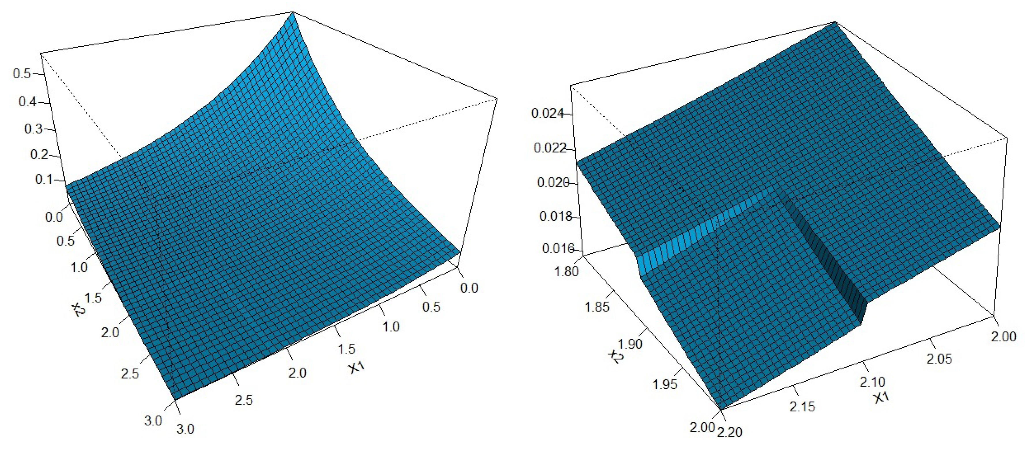
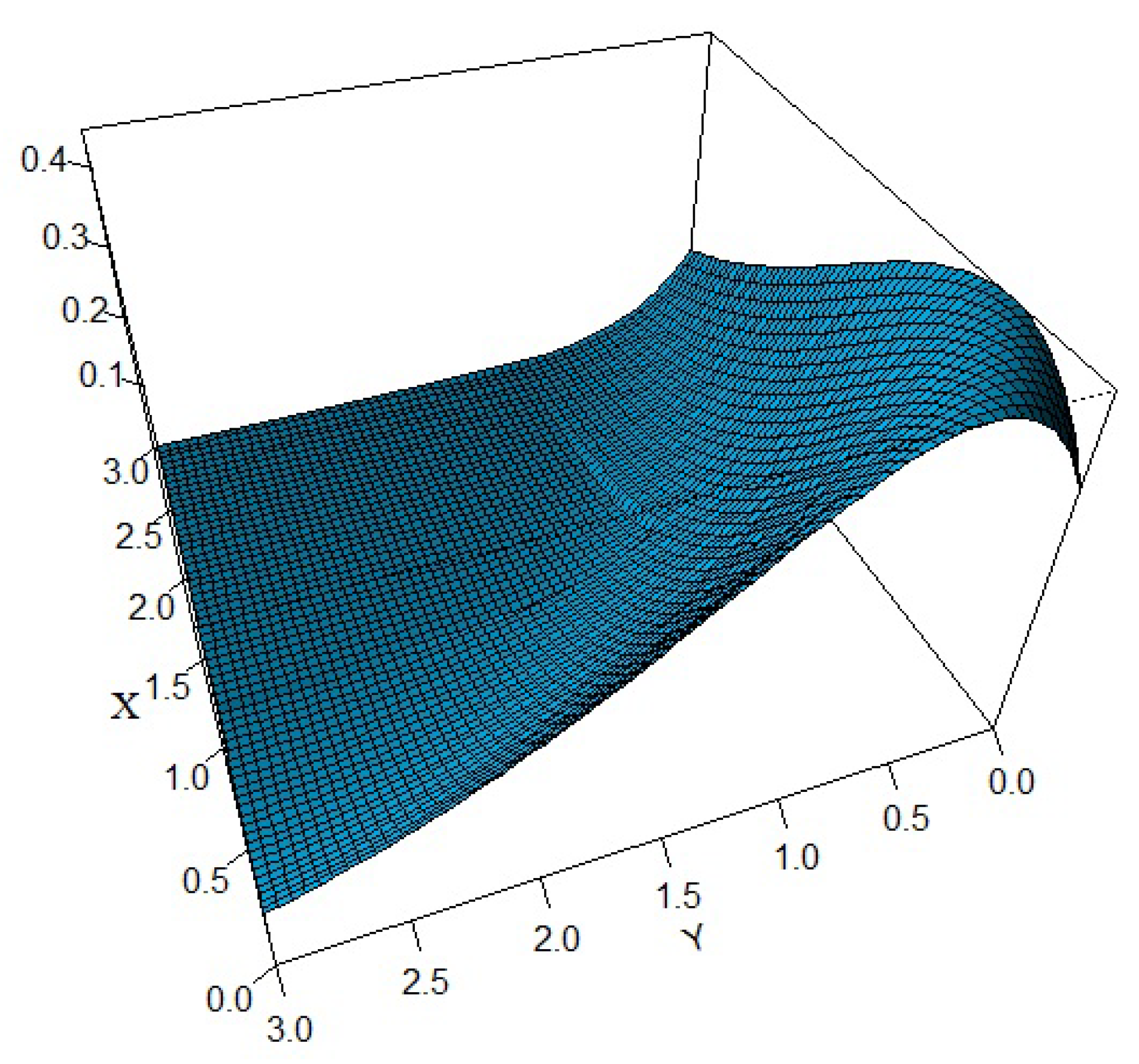
4. Particular Case: Bivariate Composite Gumbel–Pareto Distribution

In particular, we shall assume that $f_1$ is the pdf of a Gumbel bivariate exponential distribution truncated on the domain D, and that $f_2$ is a bivariate Pareto pdf defined on $D_{22}$, which is left truncated by its nature. Therefore, let ${\theta }_1>0,{\theta }_2>0,$ and let $\mathbf{Y}=\left(Y_1,Y_2\right)$ follow Gumbel’s bivariate distribution (1) truncated on the domain $D,$ with parameters ${\lambda }_1,{\lambda }_2>0,\beta \in \left[0,1\right],$ and having pdf

$$f_1\left(x_1,x_2\right)=\frac{g_{\mathbf{Y}}\left(x_1,x_2\right)}{P_D},\left(x_1,x_2\right)\in D.$$

Additionally, let $\mathbf{Z}=\left(Z_1,Z_2\right)\sim Pa{I}_2\left(a,{\theta }_1,{\theta }_2\right),a>0.$ Then, using $P_D$ from (3), the pdf (6) of $\mathbf{X}$ becomes

$$f\left(x_1,x_2\right)=\left\{\begin{array}{c}r\frac{{\lambda }_1{\lambda }_2{e}^{-\left({\lambda }_1{x}_1+{\lambda }_2{x}_2+\beta {\lambda }_1{\lambda }_2{x}_1{x}_2\right)}}{1-e^{-\left({\lambda }_1{\theta }_1+{\lambda }_2{\theta }_2+\beta {\lambda }_1{\lambda }_2{\theta }_1{\theta }_2\right)}}\left[\left(1+\beta {\lambda }_1{x}_1\right)\left(1+\beta {\lambda }_2{x}_2\right)-\beta \right],\left(x_1,x_2\right)\in D\hfill \\ \left(1-r\right)a\left(a+1\right)\frac{{\left({\theta }_1{\theta }_2\right)}^{a+1}}{{\left({\theta }_2{x}_1+{\theta }_1{x}_2-{\theta }_1{\theta }_2\right)}^{a+2}},\left(x_1,x_2\right)\in D_{22}\hfill \end{array}\right..$$

(10)

Note that by taking $r=0$, we obtain the bivariate Pareto pdf; with $r=1$, we obtain the bivariate Gumbel truncated on the domain D; if we take $r=1$ and ${\theta }_1={\theta }_2=0$, (10) reduces to the usual Gumbel pdf. If $\beta =0$, the Gumbel component becomes the bivariate exponential with independent marginals.

If we impose the continuity condition at $\left({\theta }_1,{\theta }_2\right)$, we obtain the following formula of r

$$r={\left(1+\frac{g_{\mathbf{Y}}\left({\theta }_1,{\theta }_2\right)}{f_2\left({\theta }_1,{\theta }_2\right)P_D}\right)}^{-1}={\left(1+\frac{\left(1+\beta {\lambda }_1{\theta }_1\right)\left(1+\beta {\lambda }_2{\theta }_2\right)-\beta }{\left(e^{{\lambda }_1{\theta }_1+{\lambda }_2{\theta }_2+\beta {\lambda }_1{\lambda }_2{\theta }_1{\theta }_2}-1\right)\left(a+1\right)a}{\lambda }_1{\lambda }_2{\theta }_1{\theta }_2\right)}^{-1}.$$

(11)

In the left side of Figure 1, we plotted a composite Gumbel–Pareto pdf satisfying marginal continuity conditions and the continuity condition at $\left({\theta }_1,{\theta }_2\right)$; see (iii) in Proposition 2. However, as discussed above, this pdf is not continuous everywhere; e.g., the continuity condition (8) becomes, in this case, $\frac{r}{P_D}{g}_{\mathbf{Y}}\left({\theta }_1,x_2\right)=(1-r)f_{\mathbf{Z}}\left({\theta }_1,x_2\right),$ which, given the pdfs $g_{\mathbf{Y}}$ and $f_{\mathbf{Z}}$, cannot be satisfied for all $x_2>{\theta }_2$. This can be seen from the right plot of the same figure, where we focused better on the threshold lines $\left\{x_1={\theta }_1,x_2>{\theta }_2\right\}$ and $\left\{x_1>{\theta }_1,x_2={\theta }_2\right\}$.

Figure 1. Left: composite Gumbel–Pareto pdf with continuous marginals and continuity at $\left({\theta }_1,{\theta }_2\right)$; Right: zoom of the same pdf (parameters: ${\lambda }_1=0.81,{\lambda }_2=0.9,\beta =0.2,a=1.0258,{\theta }_1=2.1,{\theta }_2=1.89$).

In Figure 2, we plotted another composite Gumbel–Pareto pdf with different parameters and all continuity conditions, having a more heavy-tailed Pareto component ($a<1$). A certain flexibility of the pdf’s shape can be noticed from the two plots. However, in both pdf plots, note the areas of strong decrease for small values of $x_1$ and $x_2$ due to the exponential characteristic of the Gumbel distribution.

Figure 2. Composite Gumbel–Pareto pdf with continuous marginals and continuity at $\left({\theta }_1,{\theta }_2\right)$ (parameters: ${\lambda }_1=1,{\lambda }_2=1.2,\beta =0.7,a=0.7515,{\theta }_1=1.2,{\theta }_2=1)$.

We also plotted in Figure 3 the marginal pdfs of the two composite Gumbel–Pareto distributions considered in Figure 1 and Figure 2, and we note their continuity and exponential type shapes for small values of x.

Figure 3. Marginal pdfs of composite Gumbel–Pareto distribution: left—with parameters from Figure 1; right—with parameters from Figure 2 ($f_{X_1}$ solid line, $f_{X_2}$ dashed line).

4.1. Some Properties

The marginal distributions of $\mathbf{X}$ are both of univariate composite type, having a standard exponential pdf up to the threshold.

Proposition 1. 

(i) For the composite Gumbel–Pareto distribution, the marginal pdfs of $X_1$ and $X_2$ are given by

$$\begin{array}{ccc}\hfill f_{X_1}\left(x_1\right)& =& \left\{\begin{array}{c}\frac{r}{P_D}{\lambda }_1{e}^{-{\lambda }_1{x}_1},0<x_1\le {\theta }_1\hfill \\ \frac{r}{P_D}{\lambda }_1{e}^{-{\lambda }_1{x}_1}\left[1-\left(1+\beta {\lambda }_2{\theta }_2\right)e^{-{\lambda }_2{\theta }_2\left(1+\beta {\lambda }_1{x}_1\right)}\right]+\left(1-r\right)a\frac{{\theta }_1^a}{x_1^{a+1}},x_1>{\theta }_1\hfill \end{array}\right.,\hfill \\ \hfill f_{X_2}\left(x_2\right)& =& \left\{\begin{array}{c}\frac{r}{P_D}{\lambda }_2{e}^{-{\lambda }_2{x}_2},0<x_2\le {\theta }_2\hfill \\ \frac{r}{P_D}{\lambda }_2{e}^{-{\lambda }_2{x}_2}\left[1-\left(1+\beta {\lambda }_1{\theta }_1\right)e^{-{\lambda }_1{\theta }_1\left(1+\beta {\lambda }_2{x}_2\right)}\right]+\left(1-r\right)a\frac{{\theta }_2^a}{x_2^{a+1}},x_2>{\theta }_2\hfill \end{array}\right..\hfill \end{array}$$

(ii) Further, the cdfs of $X_1$ and $X_2$ are

$$\begin{array}{ccc}\hfill F_{X_1}\left(x_1\right)& =& \left\{\begin{array}{c}\frac{r}{P_D}\left(1-e^{-{\lambda }_1{x}_1}\right),0<x_1\le {\theta }_1\hfill \\ 1+\frac{r}{P_D}{e}^{-{\lambda }_1{x}_1}\left(e^{-{\lambda }_2{\theta }_2(1+\beta {\lambda }_1{x}_1)}-1\right)-\left(1-r\right){\left(\frac{{\theta }_1}{x_1}\right)}^a,x_1>{\theta }_1\hfill \end{array}\right.,\hfill \\ \hfill F_{X_2}\left(x_2\right)& =& \left\{\begin{array}{c}\frac{r}{P_D}\left(1-e^{-{\lambda }_2{x}_2}\right),0<x_2\le {\theta }_2\hfill \\ 1+\frac{r}{P_D}{e}^{-{\lambda }_2{x}_2}\left(e^{-{\lambda }_1{\theta }_1(1+\beta {\lambda }_2{x}_2)}-1\right)-\left(1-r\right){\left(\frac{{\theta }_2}{x_2}\right)}^a,x_2>{\theta }_2\hfill \end{array}\right..\hfill \end{array}$$

We can impose marginal continuity conditions and combine them with the continuity condition at $\left({\theta }_1,{\theta }_2\right)$. The following restrictions result.

Proposition 2. 

Let $\mathbf{X}$ follow the bivariate composite Gumbel–Pareto distribution. Then:

(i) 

By imposing the continuity condition to the marginal $X_1,$ we obtain

$$r_1={\left(1+\frac{{\lambda }_1{\theta }_1}{a}\frac{1+\beta {\lambda }_2{\theta }_2}{e^{{\lambda }_1{\theta }_1+{\lambda }_2{\theta }_2+\beta {\lambda }_1{\lambda }_2{\theta }_1{\theta }_2}-1}\right)}^{-1}.$$

(ii) 

By imposing the continuity condition to the marginal $X_2,$ we obtain

$$r_2={\left(1+\frac{{\lambda }_2{\theta }_2}{a}\frac{1+\beta {\lambda }_1{\theta }_1}{e^{{\lambda }_1{\theta }_1+{\lambda }_2{\theta }_2+\beta {\lambda }_1{\lambda }_2{\theta }_1{\theta }_2}-1}\right)}^{-1}.$$

(iii) 

By simultaneously imposing continuity conditions to the marginals $X_1$ and $X_2,$ we obtain

$${\lambda }_1{\theta }_1={\lambda }_2{\theta }_2.$$

If, moreover, we also impose the continuity condition at $\left({\theta }_1,{\theta }_2\right),$ the following restriction must be fulfilled    

$$\begin{array}{c}\hfill a={\lambda }_1{\theta }_1\left(1+\beta {\lambda }_1{\theta }_1-\frac{\beta }{1+\beta {\lambda }_1{\theta }_1}\right)-1.\end{array}$$

Proposition 3. 

(i) The expected values of the marginals are given for $a>1$ by

$$\begin{array}{ccc}\hfill \mathbb{E}{X}_1& =& \frac{r}{{\lambda }_1{P}_D}\left[1-e^{-\left({\lambda }_1{\theta }_1+{\lambda }_2{\theta }_2+\beta {\lambda }_1{\lambda }_2{\theta }_1{\theta }_2\right)}\left(\frac{1}{1+\beta {\lambda }_2{\theta }_2}+{\lambda }_1{\theta }_1\right)\right]+\left(1-r\right)\frac{a{\theta }_1}{a-1},\hfill \\ \hfill \mathbb{E}{X}_2& =& \frac{r}{{\lambda }_2{P}_D}\left[1-e^{-\left({\lambda }_1{\theta }_1+{\lambda }_2{\theta }_2+\beta {\lambda }_1{\lambda }_2{\theta }_1{\theta }_2\right)}\left(\frac{1}{1+\beta {\lambda }_1{\theta }_1}+{\lambda }_2{\theta }_2\right)\right]+\left(1-r\right)\frac{a{\theta }_2}{a-1}.\hfill \end{array}$$

(ii) The second-order moments of the marginals are given for $a>2$ by

$$\begin{array}{ccc}\hfill \mathbb{E}\left[X_1^2\right]& =& \frac{r}{{\lambda }_1^2{P}_D}\left[2-e^{-\left({\lambda }_1{\theta }_1+{\lambda }_2{\theta }_2+\beta {\lambda }_1{\lambda }_2{\theta }_1{\theta }_2\right)}\frac{1+{\left({\lambda }_1{\theta }_1\left(1+\beta {\lambda }_2{\theta }_2\right)+1\right)}^2}{{\left(1+\beta {\lambda }_2{\theta }_2\right)}^2}\right]+\left(1-r\right)\frac{a{\theta }_1^2}{a-2},\hfill \\ \hfill \mathbb{E}\left[X_2^2\right]& =& \frac{r}{{\lambda }_2^2{P}_D}\left[2-e^{-\left({\lambda }_1{\theta }_1+{\lambda }_2{\theta }_2+\beta {\lambda }_1{\lambda }_2{\theta }_1{\theta }_2\right)}\frac{1+{\left({\lambda }_2{\theta }_2\left(1+\beta {\lambda }_1{\theta }_1\right)+1\right)}^2}{{\left(1+\beta {\lambda }_1{\theta }_1\right)}^2}\right]+\left(1-r\right)\frac{a{\theta }_2^2}{a-2}.\hfill \end{array}$$

Proposition 4. 

The expected value of the product $X_1{X}_2$ is

$$\begin{array}{ccc}\hfill \mathbb{E}\left[X_1{X}_2\right]& =& \frac{r}{P_D\beta {\lambda }_1{\lambda }_2}\left[\left(E_1\left(\frac{1}{\beta }\right)-E_1\left(\frac{\left(1+\beta {\lambda }_1{\theta }_1\right)\left(1+\beta {\lambda }_2{\theta }_2\right)}{\beta }\right)\right)e^{\frac{1}{\beta }}\right.\hfill \\ & & \left.-\left(2-\frac{1}{1+\beta {\lambda }_1{\theta }_1}-\frac{1}{1+\beta {\lambda }_2{\theta }_2}+\beta {\lambda }_1{\lambda }_2{\theta }_1{\theta }_2\right)e^{-\left({\lambda }_1{\theta }_1+{\lambda }_2{\theta }_2+\beta {\lambda }_1{\lambda }_2{\theta }_1{\theta }_2\right)}\right]\hfill \\ & & +(1-r){\theta }_1{\theta }_2\frac{a^2-a-1}{(a-1)(a-2)}.\hfill \end{array}$$

In view of the random generation procedure, we also need the following result on the conditional distribution of a marginal.

Proposition 5. 

The conditional cdf of the marginal $X_2$ given $X_1=x_1$ is

$$F_{X_2|X_1=x_1}\left(x_2\right)=\left\{\begin{array}{c}1-e^{-{\lambda }_2{x}_2\left(1+\beta {\lambda }_1{x}_1\right)}\left(1+\beta {\lambda }_2{x}_2\right),x_1\le {\theta }_1,x_2>0\hfill \\ \frac{r}{P_D}{\lambda }_1{e}^{-{\lambda }_1{x}_1}\frac{1-e^{-{\lambda }_2{x}_2\left(1+\beta {\lambda }_1{x}_1\right)}\left(1+\beta {\lambda }_2{x}_2\right)}{\frac{r}{P_D}{\lambda }_1{e}^{-{\lambda }_1{x}_1}\left[1-\left(1+\beta {\lambda }_2{\theta }_2\right)e^{-{\lambda }_2{\theta }_2\left(1+\beta {\lambda }_1{x}_1\right)}\right]+\left(1-r\right)a\frac{{\theta }_1^a}{x_1^{a+1}}},x_1>{\theta }_1,x_2\le {\theta }_2\hfill \\ 1-\left(1-r\right)\frac{a{\theta }_1^a{\theta }_2^{a+1}{\left({\theta }_1{x}_2+{\theta }_2{x}_1-{\theta }_1{\theta }_2\right)}^{-(a+1)}}{\frac{r}{P_D}{\lambda }_1{e}^{-{\lambda }_1{x}_1}\left[1-\left(1+\beta {\lambda }_2{\theta }_2\right)e^{-{\lambda }_2{\theta }_2\left(1+\beta {\lambda }_1{x}_1\right)}\right]+\left(1-r\right)a\frac{{\theta }_1^a}{x_1^{a+1}}},x_1>{\theta }_1,x_2>{\theta }_2\hfill \end{array}\right..$$

4.2. Simulation

We propose two methods for generating random values from the bivariate composite Gumbel–Pareto distribution. The first one is the inversion method, while the second one is based on the representation in expression (7).

Method I: In the bivariate case, the inversion method consists of two steps:

1.

Generate a value $x_1$ from the marginal distribution of $X_1$ by inverting its cdf given in Proposition 1;

2.

Generate a value $x_2$ from the conditional distribution of $X_2$ given $X_1=x_1$ by inverting the conditional cdf given in Proposition 5. Thus, the resulting pair $\left(x_1,x_2\right)$ is simulated from (10).

Method II: Starting from the two-component mixture representation (7) with mixing weights r and $1-r$, we propose the following algorithm:

1.

Generate a value b from the Bernoulli distribution with parameter r;

2.

If $b=1$, then generate the pair $\left(x_1,x_2\right)$ from the Gumbel distribution truncated on D;

3.

If $b=0$, then generate the pair $\left(x_1,x_2\right)$ from the bivariate Pareto distribution (4).

Now the problem is to generate values from the two bivariate distributions: Gumbel and Pareto. Bivariate Pareto values can be generated without difficulty by the inversion method as described in Method I. Concerning the Gumbel distribution truncated on D, the following cdfs (obtained similarly to the ones in Propositions 1 and 5) can be used for inversion:

The cdf of the truncated Gumbel marginal, $Y_1^D$:

$$F_{Y_1^D}\left(x_1\right)=\left\{\begin{array}{c}\frac{1}{P_D}\left(1-e^{-{\lambda }_1{x}_1}\right),0<x_1\le {\theta }_1\hfill \\ 1+\frac{1}{P_D}{e}^{-{\lambda }_1{x}_1}\left(e^{-{\lambda }_2{\theta }_2(1+\beta {\lambda }_1{x}_1)}-1\right),x_1>{\theta }_1\hfill \end{array}\right.;$$

The conditional cdf of the marginal $Y_2^D$ given $Y_1^D=x_1$ of the truncated Gumbel distribution:

$$F_{Y_2^D|Y_1^D=x_1}\left(x_2\right)=\left\{\begin{array}{c}1-\left(1+\beta {\lambda }_2{x}_2\right)e^{-{\lambda }_2{x}_2\left(1+\beta {\lambda }_1{x}_1\right)},x_1\le {\theta }_1\hfill \\ \frac{1-\left(1+\beta {\lambda }_2{x}_2\right)e^{-{\lambda }_2{x}_2\left(1+\beta {\lambda }_1{x}_1\right)}}{1-\left(1+\beta {\lambda }_2{\theta }_2\right)e^{-{\lambda }_2{\theta }_2\left(1+\beta {\lambda }_1{x}_1\right)}},x_1>{\theta }_1\hfill \end{array}\right.,x_2>0.$$

4.3. Parameter Estimation

For a univariate composite distribution, estimating the parameters is already a difficult problem because the threshold where the distribution changes shape is itself a parameter. Therefore, the usual approach in the univariate case consists of sorting the data, assuming that the threshold lies between each two consecutive data points, and finding the corresponding MLE solution; then, the best MLE solution is selected from among the available ones. Alternatively, a set of possible thresholds can be defined, and for each such value, the resulting likelihood is maximized; see also the review [11] for threshold estimation approaches.

In the bivariate case, the estimation problem becomes even more difficult because there are two unknown thresholds ${\theta }_1,{\theta }_2$ to estimate. Let $\mathbf{x}={\left(x_{1i},x_{2i}\right)}_{i=1}^n$ be a bivariate data sample of size n, let ${\lambda }_1,{\lambda }_2,\beta ,a,r$ denote the rest of the parameters of the bivariate density defined in (10) (note that r might be obtained from a continuity condition such as (11) or the ones in Proposition 2, if imposed), and let L denote the likelihood function

$$L\left(\mathbf{x};{\lambda }_1,{\lambda }_2,\beta ,a,{\theta }_1,{\theta }_2,r\right)=\prod _{\left\{\left(x_{1i},x_{2i}\right)\in D\right\}}r{f}_1\left(x_1,x_2\right)\prod _{\left\{\left(x_{1i},x_{2i}\right)|x_{1i}>{\theta }_1,x_{2i}>{\theta }_2\right\}}(1-r)f_2\left(x_1,x_2\right).$$

(12)

The log-likelihood function defined from (12) is the weighted sum of the two partial log-likelihood functions associated with the two distributions of the composite model: the Gumbel and the Pareto. Since the MLE exists for both distributions (see [10] for the bivariate Pareto distribution), then for a known r, we can easily find the MLE of our composite model. The aim of the proposed MLE procedures is to find the best value of r.

In the following, we propose two alternative methods to estimate the parameters.

Method 1: An approach similar to the one described in the univariate case would be to sort the marginal data, obtaining ${\left(x_{1\left(i\right)}\right)}_{i=1}^n$ and ${\left(x_{2\left(i\right)}\right)}_{i=1}^n$, assume that each threshold lies, correspondingly, between each two consecutive marginal data points, find the MLEs, and choose the best one. However, this procedure is very time-consuming in the bivariate case, so we propose to combine it with marginal estimation in a two-part method as follows:

I.

Perform marginal estimation for both marginals; since the marginals are univariate composite distributions, the approach described above for the univariate case can be used. This would give starting values for the marginal parameters and the approximate location of the marginally estimated thresholds $\widetilde{{\theta }_1},\widetilde{{\theta }_2}$.

II.

Let ${\left(x_{1\left(i\right)}\right)}_{i=1}^n$ and ${\left(x_{2\left(i\right)}\right)}_{i=1}^n$ denote the (increasing) sorted marginal data and assume that the marginally estimated thresholds $\widetilde{{\theta }_j}\in m_{j\left(k_j\right)},j=1,2$, where $m_{j\left(k_j\right)}=\left(x_{j\left(k_j\right)},x_{j(k_j+1)}\right)$. Now consider ${\left(m_{j(k_j-h)}\right)}_{h=1}^l$ the l intervals preceding and ${\left(m_{j(k_j+h)}\right)}_{h=1}^l$ the l intervals following the interval $m_{j\left(k_j\right)}$ that covers $\widetilde{{\theta }_j},j=1,2$, as long as they exist; for each combination of such intervals, perform full MLE and keep the best solution. The resulting algorithm is:

• Step 1. For $m_{j(k_j-l)}$ to $m_{j(k_j+l)}$, $j=1,2$,
  evaluate ${\lambda }_1,{\lambda }_2,\beta ,a,{\theta }_1,{\theta }_2,r$ as solutions of the optimization problem:

  $$maxlogL\left(\mathbf{x};{\lambda }_1,{\lambda }_2,\beta ,a,{\theta }_1,{\theta }_2,r\right),$$

  under the constraints ${\theta }_1$ and ${\theta }_2$ in the corresponding intervals, and continuity conditions, if imposed.
• Step 2. Among the solutions obtained from Step 1, choose the one that maximizes the log-likelihood function.

Note that in this way, for reasonable choices of $m_{1\left(k_1\right)},m_{2\left(k_2\right)}$ and l, the computing time is significantly reduced.

Method 2: The second method is a more analytical procedure for a specific sample; it takes into account that the parameter $\beta$ of the bivariate Gumbel–Pareto density (10) is restricted to the $[0,1]$ interval. This allows us to define a grid for it and to optimize the rest of the parameters for each value in this grid. The following procedure is designed, assuming the continuity conditions given in (i–iii) of Proposition 2 and the conditional likelihood defined by:

$$L^c\left(\mathbf{x};{\lambda }_1,{\theta }_1,{\theta }_2|\beta \right)=\prod _{\left\{\left(x_{1i},x_{2i}\right)\in D\right\}}r{f}_1\left(x_1,x_2\right)\prod _{\left\{\left(x_{1i},x_{2i}\right)|x_{1i}>{\theta }_1,x_{2i}>{\theta }_2\right\}}(1-r)f_2\left(x_1,x_2\right),$$

with the continuity conditions (constraints)

$$\begin{array}{ccc}\hfill {\lambda }_2& =& \frac{{\lambda }_1{\theta }_1}{{\theta }_2},\hfill \\ \hfill a& =& {\lambda }_1{\theta }_1\left(1+\beta {\lambda }_1{\theta }_1-\frac{\beta }{1+\beta {\lambda }_1{\theta }_1}\right)-1,\hfill \\ \hfill \beta & \in & \left[0,1\right).\hfill \end{array}$$

The conditional likelihood $L^c\left(\mathbf{x};{\lambda }_2,{\theta }_1,{\theta }_2|\beta \right)$ is defined similarly. The procedure for maximizing $log{L}^c\left(\mathbf{x};{\lambda }_1,{\theta }_1,{\theta }_2|\beta \right)$ is described below:

• Step 1. Obtain initial values for the parameters ${\theta }_1$, ${\theta }_2$, and ${\lambda }_1$ as follows:

  -

  The initially estimated thresholds are ${\tilde{\theta }}_1=x_{1\left(\left[n{p}_1\right]\right)}$ and ${\tilde{\theta }}_2=x_{2\left(\left[n{p}_2\right]\right)}$, where $p_j$, $j=1,2$, are two given large proportions, and $[·]$ denotes the integer part. An initial value for each proportion can be deduced from the Hill plot or by doing MLE of the univariate Pareto for the tail.

  -

  The initially estimated value of the exponential parameter ${\tilde{\lambda }}_1$ is obtained by MLE of the univariate truncated exponential distribution with density function:

  $$f\left(x_1|x_1\le {\tilde{\theta }}_1\right)=\frac{f_{X_1}\left(x_1\right)}{F_{X_1}\left({\tilde{\theta }}_1\right)}=\frac{{\lambda }_1{e}^{-{\lambda }_1{x}_1}}{1-e^{-{\lambda }_1{\tilde{\theta }}_1}}.$$

• Step 2. Define a grid for $\beta \in [0,1)$, i.e., ${\left({\beta }_g\right)}_{g=1}^G$. For each ${\beta }_g$, the estimated parameters ${\widehat{\theta }}_1^g$, ${\widehat{\theta }}_2^g$, and ${\widehat{\lambda }}_1^g$ are obtained by maximizing the conditional log-likelihood function $log{L}_g^c\left(\mathbf{x};{\lambda }_1,{\theta }_1,{\theta }_2|{\beta }_g\right)$. The optim() function of R software with the “Nelder–Mead” method can be used; this works reasonably well for non-differentiable functions. The parameters ${\widehat{\lambda }}_2^g$ and ${\widehat{a}}^g$ are estimated using the continuity conditions.
• Step 3. Let ${(log{\tilde{L}}_g^c)}_{g=1}^G$ be the optimal values of the log-likelihood obtained at Step 2, and let $\left({\widehat{\lambda }}_1^g,{\widehat{\theta }}_1^g,{\widehat{\theta }}_2^g,{\beta }_g\right)$ be the corresponding parameters. The final estimated parameters are:

  $$\left({\widehat{\lambda }}_1,{\widehat{\theta }}_1,{\widehat{\theta }}_2,\widehat{\beta }\right)=arg\underset{g=1,...,G}{max}log{\tilde{L}}_g^c$$

  with

  $${\widehat{\lambda }}_2=\frac{{\widehat{\lambda }}_1{\widehat{\theta }}_1}{{\widehat{\theta }}_2},$$

  $$\widehat{a}={\widehat{\lambda }}_1{\widehat{\theta }}_1\left(1+\widehat{\beta }{\widehat{\lambda }}_1{\widehat{\theta }}_1-\frac{\widehat{\beta }}{1+\widehat{\beta }{\widehat{\lambda }}_1{\widehat{\theta }}_1}\right)-1.$$

5. Numerical Illustration

In this section, we present two numerical illustrations: the first one is on simulated data, and the second one is on a real data set.

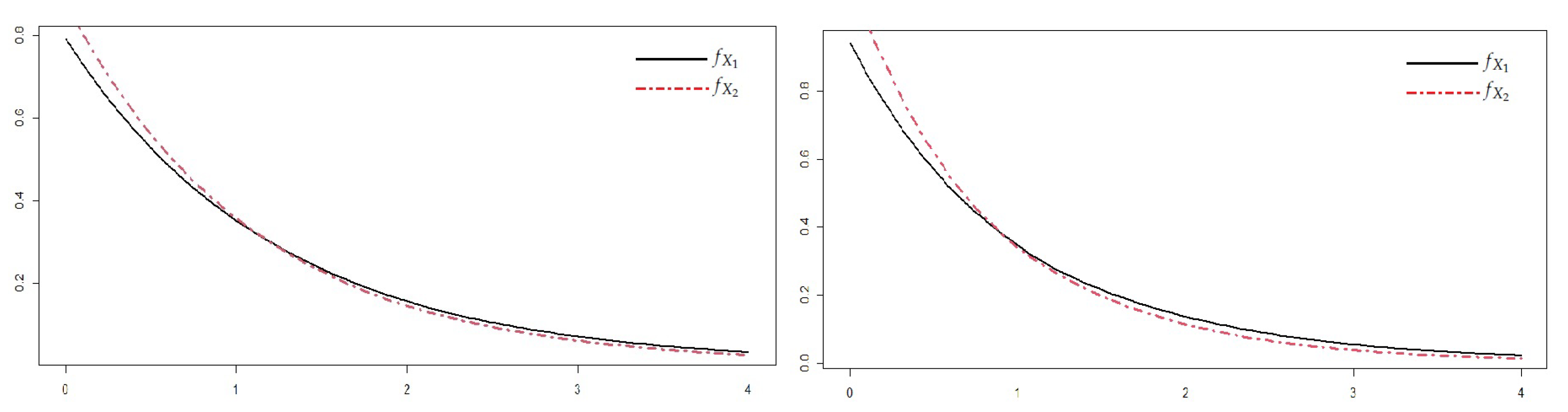
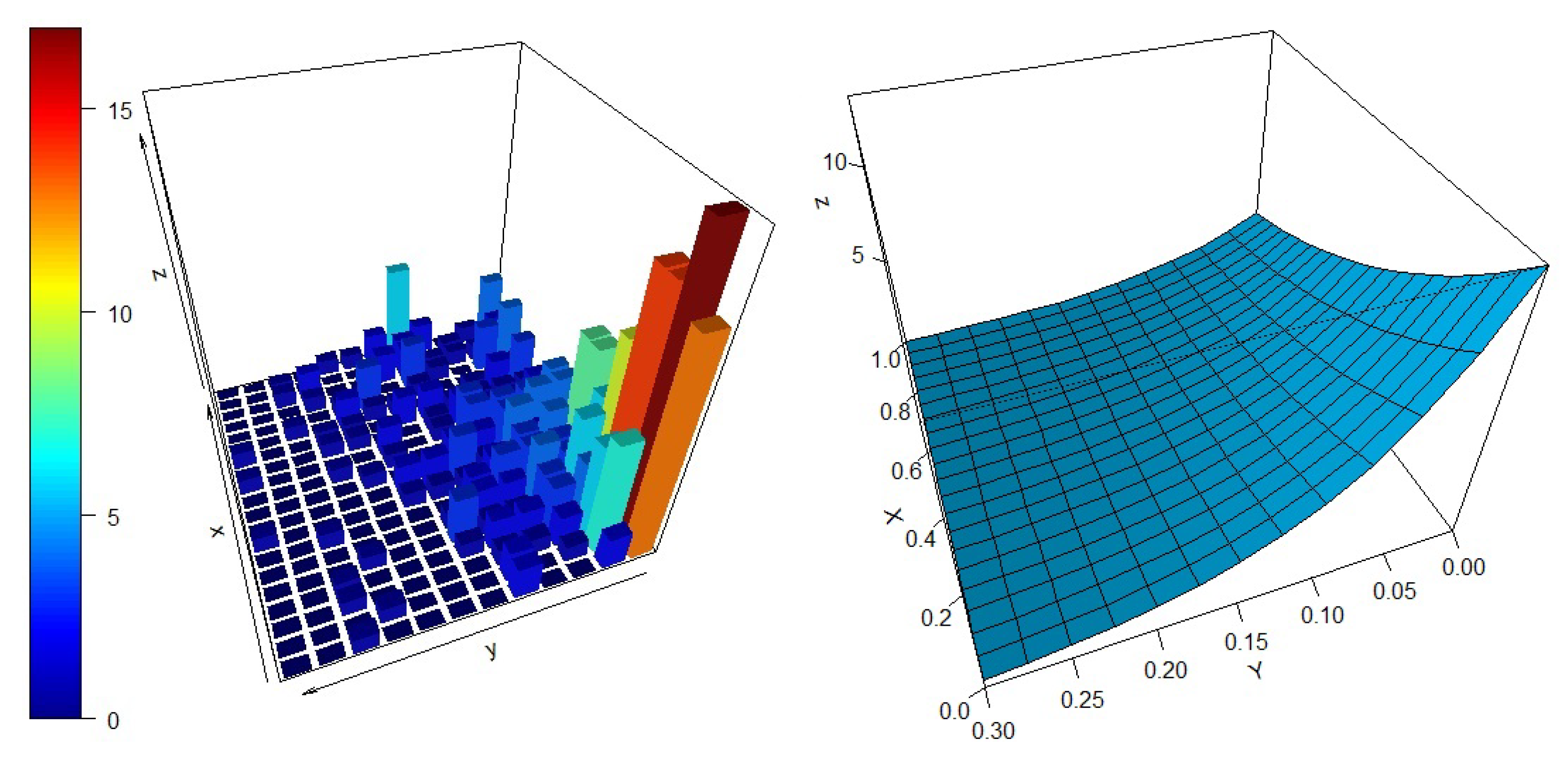
5.1. Numerical Illustration Using Simulated Data

In this section, we used simulated data to check the performance of the first estimation procedure (Method 1) proposed in Section 4.3. The true values of the parameters were selected such that they satisfied all the continuity conditions given in Proposition 2: Gumbel: ${\lambda }_1=1,{\lambda }_2=1.2,\beta =0.7;$ Pareto: $a=0.7515,{\theta }_1=1.2,{\theta }_2=1$, while $r=0.9086,P_D=0.9669$. Note that due to the heavy-tailedness of the Pareto distribution ($a<1$), there is no expected value for this particular distribution (its pdf is plotted in Figure 2).

With the aim of studying the properties of Method 1, using the two simulation methods described in Section 4.2, we generated 100 samples of size $n=200$ and $n=$ 1000, respectively, for the two methods. For each such sample, in the first step, we performed marginal estimation by imposing the continuity condition for each marginal (which restricts the parameters r, as stated in Proposition 2). As a consequence, $\beta$ and a are estimated twice (for each marginal), and because of the differences in these estimations, we cannot rely only on marginal estimation. However, marginal estimation provides starting values for performing full MLE, and even better, gives an idea of where to look for the thresholds. More precisely, we restricted the search to about 40 intervals for each ${\theta }_j$, i.e., we took $l=20$. Thus, the computing time was significantly reduced compared to the threshold search through all data.

Finally, we estimated the Mean Square Error $MSE=\frac{1}{100}{\sum }_{i=1}^{100}{\left(\theta -\widehat{\theta }\right)}^2$ and the Mean Absolute Error $MAE=\frac{1}{100}{\sum }_{i=1}^{100}\left|\theta -\widehat{\theta }\right|$, where $\theta$ and $\widehat{\theta }$ represent the true and estimated parameters, respectively.

With the estimated parameters obtained from the 100 replicas generated with each simulation method, we obtained the MSE and the MAE that are shown in Table 1. The results indicate that both error criteria decrease when the sample size increases. Some differences between the two simulation methods can be observed (e.g., the MSE of $\beta$ is larger for simulation Method II than for simulation Method I, while the MSE of a is smaller for simulation Method II than for simulation Method I), but we believe that these differences are due to the randomness of the results, where some samples fall more in the Pareto part or in the exponential part; further simulation investigation is worthwhile, assuming that the estimation method can be modified to reduce the computing time.

Table 1. Simulation results with 100 replicas for MSE and MAE with sample sizes $n=200$ and $n=$ 1000.

	Simulation Method I
	${\lambda }_1$		${\lambda }_2$		$\beta$		a		${\theta }_1$		${\theta }_2$
n	MSE	MAE	MSE	MAE	MSE	MAE	MSE	MAE	MSE	MAE	MSE	MAE
200	0.0037	0.0538	0.0060	0.0717	0.0124	0.1077	0.3855	0.6152	0.0530	0.2226	0.0144	0.1069
1000	0.0034	0.0511	0.0048	0.0610	0.0118	0.1044	0.0275	0.1625	0.0450	0.2109	0.0049	0.0619
	Simulation Method II
	${\lambda }_1$		${\lambda }_2$		$\beta$		a		${\theta }_1$		${\theta }_2$
n	MSE	MAE	MSE	MAE	MSE	MAE	MSE	MAE	MSE	MAE	MSE	MAE
200	0.0054	0.0721	0.0041	0.0447	0.1530	0.3900	0.0640	0.2493	0.0694	0.2619	0.0985	0.3010
1000	0.0048	0.0610	0.0002	0.0131	0.1234	0.3367	0.0174	0.1267	0.0638	0.2564	0.0567	0.2229

Concerning Method 2, as already noticed, it is a more analytical procedure for a specific sample, and therefore, it cannot be standardized and we cannot perform several iterations to calculate MSE and MAE.

All the computations were preformed in R software using an optimization function with constraints to implement the continuity restrictions. The code is available upon request from the authors.

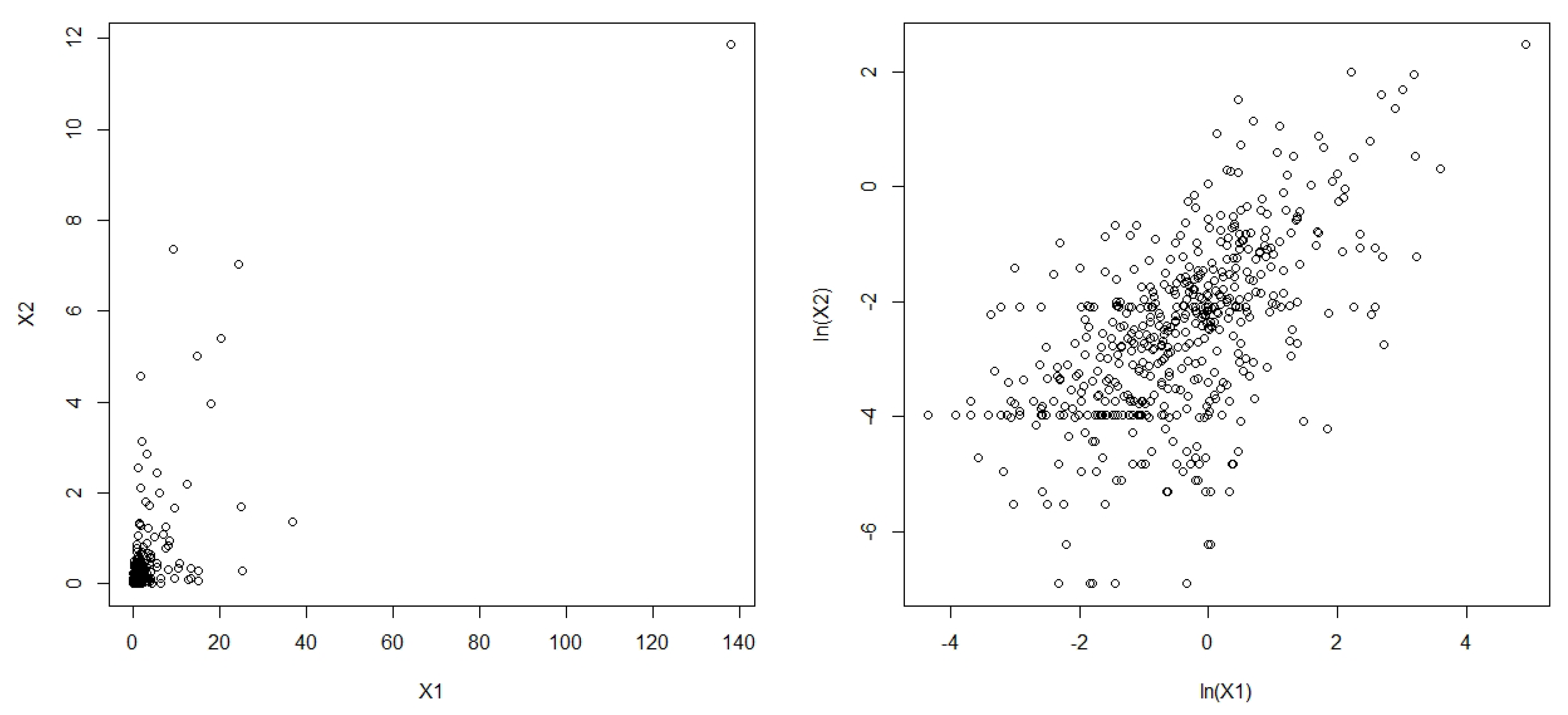
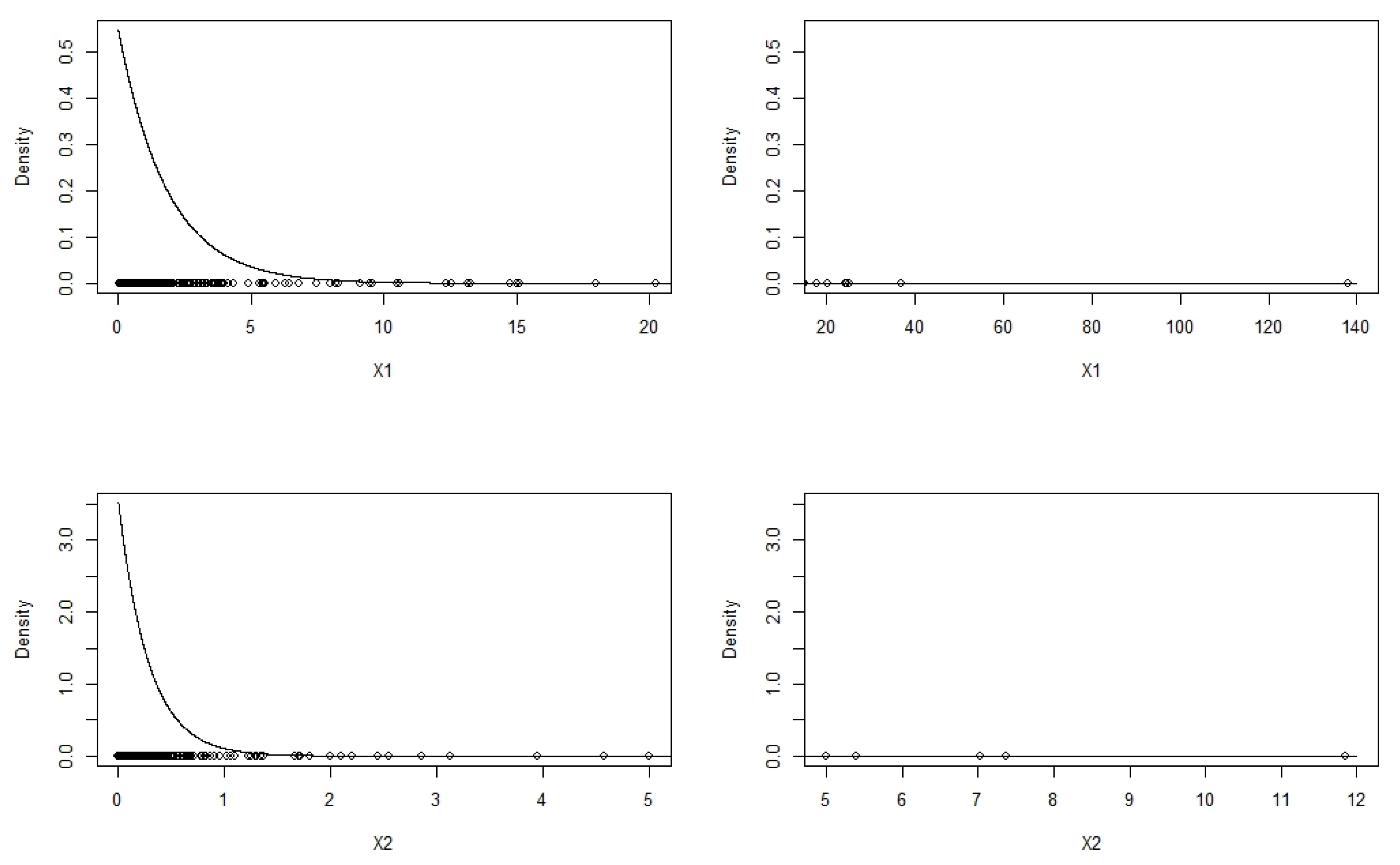
5.2. Numerical Illustration with Real Data

In this section, we fit our proposed bivariate Gumbel–Pareto distribution to a random sample of $n=518$ motor insurance claims that include bodily injury. For these claims, we separately know the cost of property damage including third-part liability (variable $X_1$) and the cost of exceptional medical expenses not covered by public social security (variable $X_2$). The data were provided by a major insurer in Spain in the year 2002 and correspond to claims that occurred in the year 2000. These data were studied in previous works (see [5,6,12]).

In Table 2, we display the descriptive statistics of the original data divided by 1000; this change of scale is convenient, and it facilitates the MLE of the parameters. These descriptive statistics show that both variables have a strong right skewness. Furthermore, the left plot in Figure 4 shows the scatterplot of both cost variables in the original scale divided by 1000, where the existence of extreme values in both variables can be noticed. When we have right-skewed variables with extreme values, the MLE of a simple distribution as, e.g., the exponential, the Weibull, or the log-normal, tends to underestimate the probability on the right tail. Figure 5 displays the univariate exponential pdf fitted by MLE to each marginal variable; with these densities, we also plotted the observed costs: on top the costs of property damage, including third-part liability, and on bottom the costs of exceptional medical expenses not covered by public social security. For better visibility, the domains of the cost variables were divided in two parts, resulting in two plots for each marginal. Figure 5 shows how the density reaches zero in the part of the domain where there are still sample observations; so clearly, this model assumes a zero probability where it should not. Similar results are obtained using univariate Weibull and log-normal densities.

Table 2. Descriptive statistics of property damage and third-party liability costs ($X_1$) and exceptional medical expenses ($X_2$).

	Mean	STD	Min	Q25	Median	Q75	Max	Kurtosis	Skewness
X1	1.83	6.87	0.01	0.26	0.68	1.39	137.94	15.70	301.30
X2	0.28	0.86	0.00	0.02	0.09	0.20	11.86	8.06	85.35

Figure 4. Scatterplots of $X_1$ vs. $X_2$ in original (left) and natural (right) logarithm scales.

Figure 5. Exponential pdf fitted by MLE and sample data shown as points on the horizontal axis for both marginals.

Therefore, the composite model with a Pareto right tail is a good way to improve the MLE fit for both univariate and bivariate data. Moreover, graphical analysis (e.g., the Hill plot) indicates that both variables have a Pareto tail with a shape parameter very close to 1, i.e., we have heavy-tailed marginal distributions. Thus, we can conclude that their distributions have only the first-order moment finite, or they do not have finite moments at all. In the left scatterplot of Figure 4, we can note that the sample information on extreme values is scarce; this is a difficulty in samples from heavy-tailed or Pareto distributions.

To asses the joint behavior of $X_1$ and $X_2$, we calculated the Pearson linear correlation and the Kendall and the Spearman rank correlation coefficients, displayed in Table 3. These results show a strong dependence between the two cost variables. However, as can be seen from Figure 4, which presents the data scatterplot in both original and natural logarithm scales, the dependence is not linear. As shown in [12], these data exhibit extreme value dependence, i.e., the higher the costs, the stronger the dependency. This behavior can also be observed in Figure 4. Furthermore, [10] shows that when the bivariate Pareto parameter a is $a\le 2$, as is the case with our cost data, the theoretical variance and covariance do not exist or cannot be calculated. Therefore, the Pearson linear correlation cannot be interpreted.

Table 3. Sample linear and rank correlation coefficients.

	Pearson	Kendall	Spearman
Correlation	0.7288	0.4252	0.5903

Further, from the right plot in Figure 4, it can be observed that for small values of both variables, the shape of the point cloud is spherical, i.e., the dependence is almost zero; however, for larger values, the shape indicates positive dependence between both variables. Clearly, this denotes a change of the joint distribution between the smaller and the larger costs.

In Table 4, we present the MLE parameters for Gumbel’s bivariate exponential distribution described in Section 2.2.1 and for the Gumbel–Pareto distribution from Section 4. The estimated parameters of the latter were obtained with Method 2 described in Section 4.3, imposing all continuity conditions (Method 1 yielded similar results). The initial values of the thresholds were taken from the Hill plots, and in this case, $p_1=p_2=0.102$, resulting in $\left[np\right]=[518\times 0.103]=52$, i.e., ${\tilde{\theta }}_1=3.1$ and ${\tilde{\theta }}_2=0.5$; also, ${\tilde{\lambda }}_1=1.4175$. Comparing the AICs, BICs, and CAICs given in Table 4 indicates that the bivariate Gumbel–Pareto clearly outperforms Gumbel’s bivariate exponential distribution. Moreover, from MLE, the dependence parameter of Gumbel’s bivariate exponential distribution, $\beta$, is zero, and it is close to zero for the Gumbel–Pareto distribution, which is coherent with the scatterplot in Figure 4.

Table 4. MLE of bivariate distributions with standard errors in parentheses.

	Gumbel	Gumbel–Pareto
${\widehat{\lambda }}_1$	0.5472 (0.0240)	1.4184 (0.0328)
${\widehat{\lambda }}_2$	3.5221 (0.1548)	11.1996
${\widehat{\theta }}_1$	-	0.9870 (0.0040)
${\widehat{\theta }}_2$	-	0.1250 (0.0003)
$\widehat{\beta }$	0.0000	0.0455 (0.0465)
a	-	0.4292
r	-	0.8303
$logL$	−696.1630	−272.5549
AIC	1398.3261	557.1097
BIC	1411.0759	582.6096
CAIC	1414.0759	588.6096

In Figure 6, we also plotted a partial histogram of the data alongside the corresponding Gumbel–Pareto pdf with the estimated parameters, while in Figure 7, we plotted the marginal histograms with the fitted pdfs.

Figure 6. Histogram of real data (left) and Gumbel–Pareto pdf with the estimated parameters (right).

Figure 7. Histogram of real data marginals with fitted pdfs: left, $X_1$; right, $X_2$.

Finally, as a risk management application, we estimated the total risk of loss for the aggregate cost random variable $S=X_1+X_2$ using Monte Carlo simulation, and based on it, we calculated the Value-at-Risk (VaR) measure. VaR is equivalent to an extreme quantile of the distribution, i.e., $Va{R}_{\alpha }\left(S\right)=inf\{s\in \mathbb{R}|Pr\left(S\le s\right)\ge \alpha \}$, where $\alpha$ is close to 1. In Table 5, we present the VaR results with $\alpha =0.95,0.99,0.995$ for: the empirical distribution of the original data, the distribution of S simulated from Gumbel’s bivariate exponential distribution, and the distribution of S simulated from the Gumbel–Pareto distribution. Furthermore, we added the VaR obtained for the bivariate log-normal distribution fitted to the data; note that this distribution underestimates the risk in a way similar to that of Gumbel’s bivariate exponential.

Table 5. Value-at-Risk for the empirical distribution and alternative distributions, obtained using Monte Carlo simulation.

	95%	99%	99.50%
Empirical	7.926	25.409	31.216
Gumbel	6.312	9.700	11.178
Gumbel–Pareto	6.361	114.067	410.897
Log-normal	6.529	15.122	20.787

When data follow a heavy-tailed distribution, the empirical VaR depends on the maximum data observed, and it is not an efficient estimator. The Gumbel–Pareto distribution provides an estimation that extrapolates beyond the observed maximum cost and takes into account the long and heavy bivariate tail with dependent marginal distributions.

6. Conclusions

To model bivariate dependent data that exhibit many small/medium values but also some very large values (i.e., extreme values), in this paper, we proposed a bivariate two-component spliced distribution. This distribution assumes a bivariate Pareto distribution on the domain consisting of values larger than some thresholds, and a bivariate Gumbel distribution on the complementary domain. We discussed some properties of the new distribution and focused on parameter estimation, proposing two alternative procedures. Because performing full MLE for this distribution may become time-prohibitive for larger data sets, as further work, we plan to investigate alternative methods that could reduce the computing time. Additionally, starting from the mixture formula (7), we plan to address the problem of parameter identifiability (see, e.g., [13] or [14]). Goodness-of-fit tests are envisaged for a future study.

Moreover, we also plan to study other such distributions by replacing the bivariate Gumbel with alternative distributions.

References

- Sarabia, J.M.; Gómez-Déniz, E. Construction of multivariate distributions: A review of some recent results. SORT 2008, 32, 3–36. [Google Scholar]
- Klugman, S.A.; Panjer, H.H.; Willmot, G.E. Loss Models: From Data to Decisions; John Wiley & Sons: New York, NY, USA, 1998. [Google Scholar]
- Scarrott, C. Univariate extreme value mixture modeling. In Extreme Value Modeling and Risk Analysis: Methods and Applications; Dipak, K.D., Jun, Y., Eds.; CRC Press: Boca Raton, FL, USA, 2016; pp. 41–67. [Google Scholar]
- Cooray, K.; Ananda, M.M. Modeling actuarial data with a composite lognormal-Pareto model. Scand. Actuar. J. 2005, 5, 321–334. [Google Scholar] [CrossRef]
- Bolancé, C.; Guillen, M.; Pelican, E.; Vernic, R. Skewed bivariate models and nonparametric estimation for the CTE risk measure. Insur. Math. Econ. 2008, 43, 386–393. [Google Scholar] [CrossRef]
- Bahraoui, Z.; Bolancé, C.; Pelican, E.; Vernic, R. On the bivariate Sarmanov distribution and copula. An application on insurance data using truncated marginal distributions. SORT 2015, 39, 209–230. [Google Scholar]
- Gumbel, E.J. Bivariate exponential distributions. J. Am. Stat. Assoc. 1960, 55, 698–707. [Google Scholar] [CrossRef]
- Kotz, S.; Balakrishnan, N.; Johnson, N.L. Continuous Multivariate Distributions, Volume 1: Models and Applications; John Wiley & Sons: New York, NY, USA, 2004. [Google Scholar]
- Castillo, E.; Sarabia, J.M.; Hadi, A.S. Fitting continuous bivariate distributions to data. Statistician 1997, 46, 355–369. [Google Scholar] [CrossRef]
- Mardia, K.V. Multivariate Pareto distributions. Ann. Math. Stat. 1962, 33, 1008–1015. [Google Scholar] [CrossRef]
- Scarrott, C.J.; MacDonald, A. A review of extreme value threshold estimation and uncertainty quantification. REVSTAT Stat. J. 2012, 10, 33–60. [Google Scholar]
- Bahraoui, Z.; Bolancé, C.; Pérez-Marín, A.M. Testing extreme value copulas to estimate the quantile. SORT 2014, 38, 89–102. [Google Scholar]
- Chen, J. Optimal rate of convergence for finite mixture models. Ann. Stat. 1995, 23, 221–233. [Google Scholar] [CrossRef]
- Kim, D.; Lindsay, B.G. Empirical identifiability in finite mixture models. Ann. Inst. Stat. Math. 2015, 67, 745–772. [Google Scholar] [CrossRef]
Publisher’s Note: MDPI stays neutral with regard to jurisdictional claims in published maps and institutional affiliations. |
© 2022 by the authors. Licensee MDPI, Basel, Switzerland. This article is an open access article distributed under the terms and conditions of the Creative Commons Attribution (CC BY) license (https://creativecommons.org/licenses/by/4.0/).