Abstract
Ridge regression is a popular method to solve the multicollinearity problem for both linear and non-linear regression models. This paper studied forty different ridge regression t-type tests of the individual coefficients of a linear regression model. A simulation study was conducted to evaluate the performance of the proposed tests with respect to their empirical sizes and powers under different settings. Our simulation results demonstrated that many of the proposed tests have type I error rates close to the 5% nominal level and, among those, all tests except one have considerable gain in powers over the standard ordinary least squares (OLS) t-type test. It was observed from our simulation results that seven tests based on some ridge estimators performed better than the rest in terms of achieving higher power gains while maintaining a 5% nominal size.
1. Introduction
Multicollinearity is the occurrence of high inter-correlations among independent variables in a multiple regression model. When this condition is present, it can result in unstable and unreliable regression coefficient estimates if the method of ordinary least squares is used. One of the proposed solutions to the problem of multicollinearity is the concept of ridge regression as pioneered by Hoerl and Kennard [1] They found that there is a nonzero value of k (ridge or shrinkage parameter) for which mean square error (MSE) for the ridge regression estimator is smaller than the variance of the ordinary least squares (OLS) estimator.
Estimating the shrinkage parameter (k) is a vital issue in the ridge regression model. Several researchers at different period of times have worked in this area of research and proposed different estimators for k. To mention a few, Hoerl and Kennard [1], Hoerl, Kennard and Baldwin [2], Lawless and Wang [3], Gibbons [4], Nomura [5], Kibria [6], Khalaf [7], Khalaf and Shukur [8], Alkhamisi and Shukur [9], Muniz and Kibria [10], Feras and Gore [11], Gruber [12], Muniz et al. [13], Mansson et al. [14], Hefnawy and Farag [15], Roozbeh and Arashi [16], Arashi and Valizadeh [17], Aslam [18], Asar and Karaibrahimoğlu [19], Saleh et al. [20], Asar and Erişoğlu [21], Goktas and Sevinc [22], Fallah et al. [23], Norouzirad and Arashi [24], and very recently Saleh et al. [25], among others
It is well known that, to make inference about an unknown population parameter, one may consider both confidence interval and hypothesis testing methods. However, the literature on the test statistics for testing the regression coefficients under the ridge regression model is very limited. First, Halawa and Bassiouni [26] proposed non exact t-tests for the regression coefficients under ridge regression estimation and compared empirical sizes and powers of only two tests based on the estimator of k proposed by Hoerl and Kennard [1] and Hoerl, Kennard, and Baldwin [2]. Their results evidenced that, for models with large standard errors, the ridge based t-tests have correct sizes with considerable gain in powers over those of the least squares t-test. For models with small standard errors, tests are found to be slightly exceeding the nominal level in few cases. Cule et al. [27] evaluated the performance of tests proposed by Hoerl and Kennard [1], Hoerl, Kennard, and Baldwin [2], and Lawless and Wang [3] based on linear ridge and logistic ridge regression models. Gokpinar and Ebegil [28] evaluated the performance of the t-tests based on 22 different estimators of the ridge parameter k collected from the published literature. Finally, Kibria and Banik [29] analyzed the performance of the t-tests based on 16 popular estimators of the ridge parameter.
Since different ridge regression estimators are considered by several researchers at different times and under different simulation methods and conditions, testing regression coefficients based on the basis of size (Type I error) and power properties under the ridge regression model are not comparable as a whole. Therefore, the important contribution of this paper is to make a more comprehensive comparison of a much larger ensemble of available t test statistics for testing regression coefficients. We consider in our analysis most of the ones analyzed in Gokpinar and Ebegil [28] and Kibria and Banik [29] as well as other test statistics based on other ridge estimators not included in the aforementioned studies at the same time. In total, our paper compares forty different t-tests statistics. The test statistics were compared based on the empirical type I error and the power properties following the testing procedures that are detailed in Halawa and Bassiouni [26]. These results are of interest for statistical practitioners using ridge regression in different fields of application as a guide to which test statistics to use when testing the significance of variables in their ridge regression models.
This paper is organized as follows. The proposed test statistics for the linear regression model are described in Section 2. To compare the performance of the test statistics, a simulation study is conducted in Section 3. An application is discussed in Section 4. Finally, some concluding remarks are given in Section 5.
2. Test Statistics for Regression Coefficients
Let us consider the following multiple linear regression model:
Y is an (n × 1) dimensional vector of dependent variables centered about their mean, X is an (n × q) dimensional observed matrix of the regressors centered and scaled such that is in correlation form, β is (q × 1) dimensional unknown coefficient vector, and ε is (n × 1) error vector distributed as multivariate normal with mean 0 and variance–covariance matrix , where In is an (n × n) identity matrix.
The ordinary least square estimator (OLS) of the parameter vector β is:
To test whether the i-th component of the parameter vector β is equal to zero, the following test is used based on the OLS estimator:
where is the ith component of , and is the square root of the ith diagonal element of with:
The test statistic in Equation (3) is the least square test statistic. Under the null hypothesis, it is distributed as Student t- distribution with n−q−1 degrees of freedom. However, when is ill conditioned due to multicollinearity, the least square estimator in (2) produces unstable estimators with unduly large sampling variance. Adding a constant k to the diagonal elements of improves the ill conditioned situation. This is called ridge regression. The ridge estimator of the parameter vector β is then:
where k > 0 is the ridge or shrinkage parameter.
The bias, the variance matrix, and the MSE expression of are respectively given as follows:
and is estimated as follows:
To test whether the i-th component of the parameter vector β is equal to zero, Halawa and Bassouni [26] proposed the following t-test statistic based on the ridge estimator of the parameter vector:
where is the ith element of , and is the square root of the ith diagonal element of
Under the null hypothesis, the test statistic (7) was shown to be approximately distributed as a Student t-distribution with degrees of freedom. For more details on this topic, see Halawa and Bassiouni [26], among others.
Values of the Ridge Estimator k Considered for the Test Statistic tk
Since the ridge parameter k is unknown, it needs to be estimated from observed data. This section gives the formulas for the forty different ridge regression estimators considered in our simulation study for the test statistic defined in (7). Table 1 below shows the estimators. For details on how the estimators were derived, we refer the readers to the corresponding original papers that are available in the list of references [1,2,3,4,5,6,7,8,9,10,11,12,13,14,15,16,17,18,19,20,21,22,23,24,25,26,27,28,29,30,31,32,33,34,35,36].

Table 1.
Some ridge regression estimators.
Here, is defined as:
where P is an orthonormal matrix that satisfies , and Λ is a diagonal matrix of eigenvalues (λj j = 1, 2,…, q) of . To calculate the value of test statistics, we considered each of the k values in Table 1 in Equations (4)–(7) and thus obtained 40 different values of the test statistics. Since a theoretical assessment among the test statistics was not possible, a simulation study was conducted to evaluate the performances of the suggested tests in the following section.
3. Simulation Study
Our simulation study has two parts. First, we analyzed the empirical Type I error of the tests. The test statistics that achieved the nominal size of 5% were kept, and the ones that deviated significantly from the 5% size were discarded. Then, the second part of the simulation study compared the tests statistics that achieved 5% nominal size in regards to statistical power.
3.1. Type I Error Rates Simulation Procedure
R Studio was used for all calculations of this paper. The R package lmridge was used to fit the ridge regression models. For the empirical Type I error simulation and the power of the test, we considered sample sizes n = 30, 50, 80, and 100, the number of regressors q = 4, 6, 8, 10, and 25, and the standard deviation of the error term was chosen as σ = 1. To see the effects of multicollinearity by stating the correlation matrix among the regressors, we assumed ρ = 0.80 and 0.95. An n × p matrix X was created as H Λ0.5 GT, where H is any (n × p) matrix whose columns are orthogonal, Λ is the diagonal matrix of eigenvalues of the correlation matrix, and G is the matrix of normalized eigenvectors of the correlation matrix, respectively. Following Halawa and Bassiouni [26], our study was based on the most favorable (MF) direction of β for model (1). The MF orientation of β corresponds to the largest normalized eigenvector of the matrix , which is a vector of the form . We chose not to use the least favorable orientation (LF) of β in our simulation, since all the literature available shows that both orientations give similar results in terms of Type I error and power. For a detailed explanation of MF and LF directions of β and other details of the simulation procedure, please see the paper by Halawa and Bassiouni [26].
To estimate the 5% nominal size (α = 0.05) for testing under different conditions, 5000 pseudo random vectors from N(0, σ2) were created to compute the error term in (1). Without loss of any generality, we let zero intercept for (1). Under the null model, substituting the i-th element of the considered MF β by zero, model (1) was used to find 5000 simulated vectors of Y. The estimated sizes were computed as the percentage of times the absolute values of all selected test statistics were greater than the critical value of t0.025, (n-q-1).
3.2. Type I Error Rates: Simulation Results
In Table 2 and Table 3, we recorded the empirical sizes of the tests for the MF orientation for correlation levels of 0.80 and 0.95, respectively

Table 2.
Simulated Type I errors for ρ = 0.80 and .

Table 3.
Simulated Type I errors for ρ = 0.95 and .
If the true Type I error rate is 5%, then, for a simulation based in 5000 runs, the observed Type I error will be in the following interval 95% of the times . We did not consider those tests for comparison’s purpose whose observed average Type I error was not in the above range.
Based on the above tables, we observed the following:
- (i)
- The tests based on the following ridge estimators, KVR, KKibAM, KM2, KM3, KM4, KM6, KM8, KM9, KM10, KM12, KASH, KSG1, KSG2, and KD1, have Type I errors very well above the 5% nominal size and therefore cannot be recommended.
- (ii)
- The tests based on the following ridge estimators, KM11, KNOM, and KFG, did not surpass the 5% nominal size but stayed below it—around 3% to 4%—and therefore cannot be recommended.
- (iii)
- The rest of the tests (including the test based on the ordinary least squares estimator) were, on average, very close to the nominal size of 5% for different sample sizes, number of variables, and levels of correlation analyzed. These tests were the ones that were compared in terms of statistical power.
We also carried out simulations for nominal sizes of 10% and 1%, and the behavior of the tests was consistent with what was observed for a nominal size of 5%. Those results are available upon request. However, we are including a table of simulated Type I errors for nominal size 1% and correlation level 0.95 in Table 4 so that one can verify that the behavior of the tests was consistent with the results for 5% nominal size shown before.

Table 4.
Simulated Type I errors for ρ = 0.95 and .
3.3. Statistical Power Simulation Procedure
After calculating the empirical type I error rates of the tests based on our initial forty ridge estimators, we discarded seventeen that did not have a nominal size between 4.4% and 5.6%. The remaining twenty-three test statistics were compared in terms of power. Following the paper by Gokpinar and Ebegil [28], we replaced the i-th component of the β vector by , where J is a whole positive number, and . We picked J = 6 since that value achieved approximately a power of 80% for the OLS test when q = 4, and having a sizeable power for the OLS test allowed for a better comparison with the other ones.
Based on 5000 simulation runs, the powers of the tests were computed by the proportion of times the absolute value of the test statistic exceeded the critical value t0.025, (n-q-1). All combinations of sample sizes of n = 30, 50, 100 and number of regressors q = 4, 6, 10 were considered under correlation levels of 0.80 and 0.95, respectively.
3.4. Statistical Power: Simulation Results
We recorded the empirical statistical power of the tests for the MF orientation for correlation levels of 0.8 and 0.95 in Table 5 and Table 6, respectively.

Table 5.
Powers of tests for ρ = 0.80 and α = 0.05.

Table 6.
Powers of tests for ρ = 0.95 and α = 0.05.
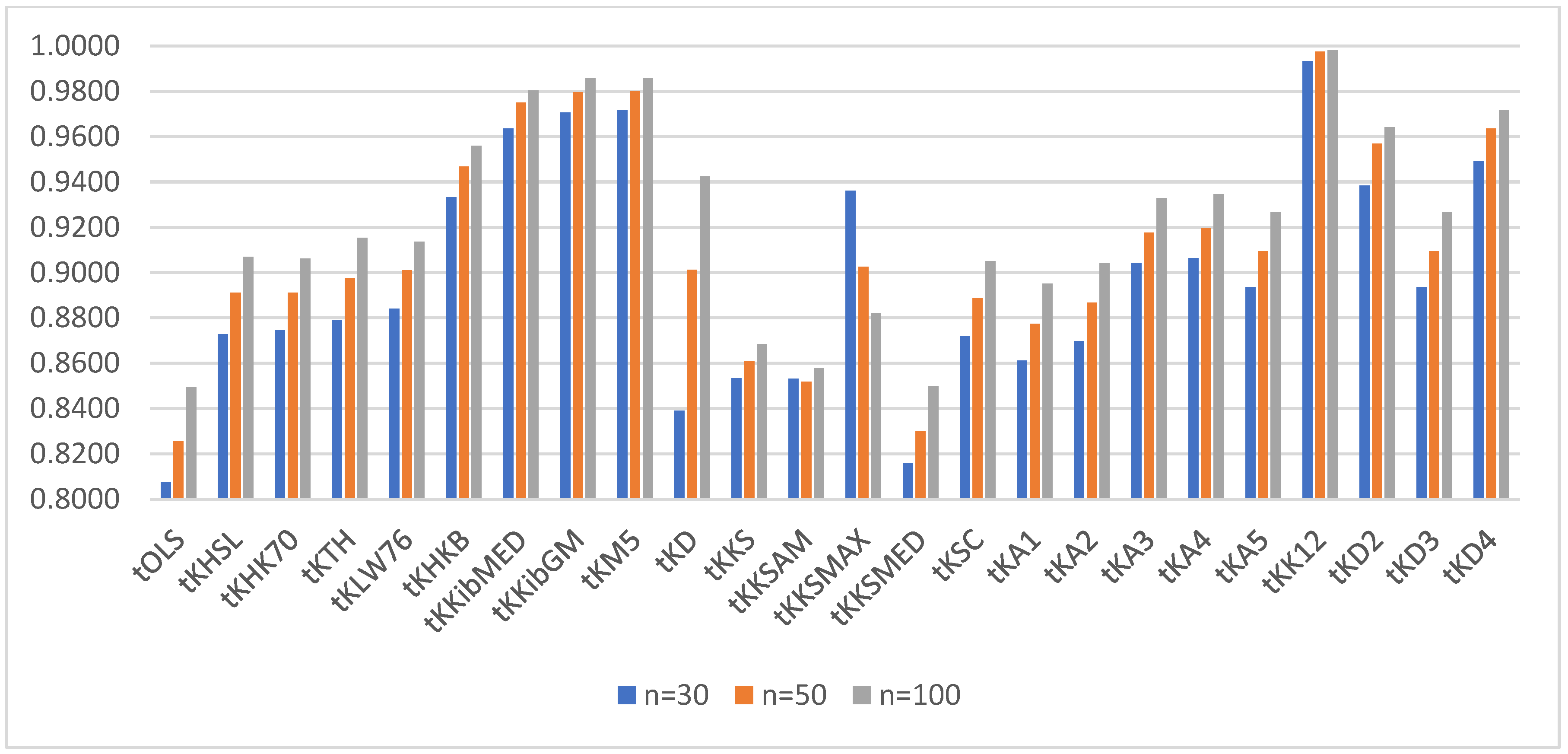
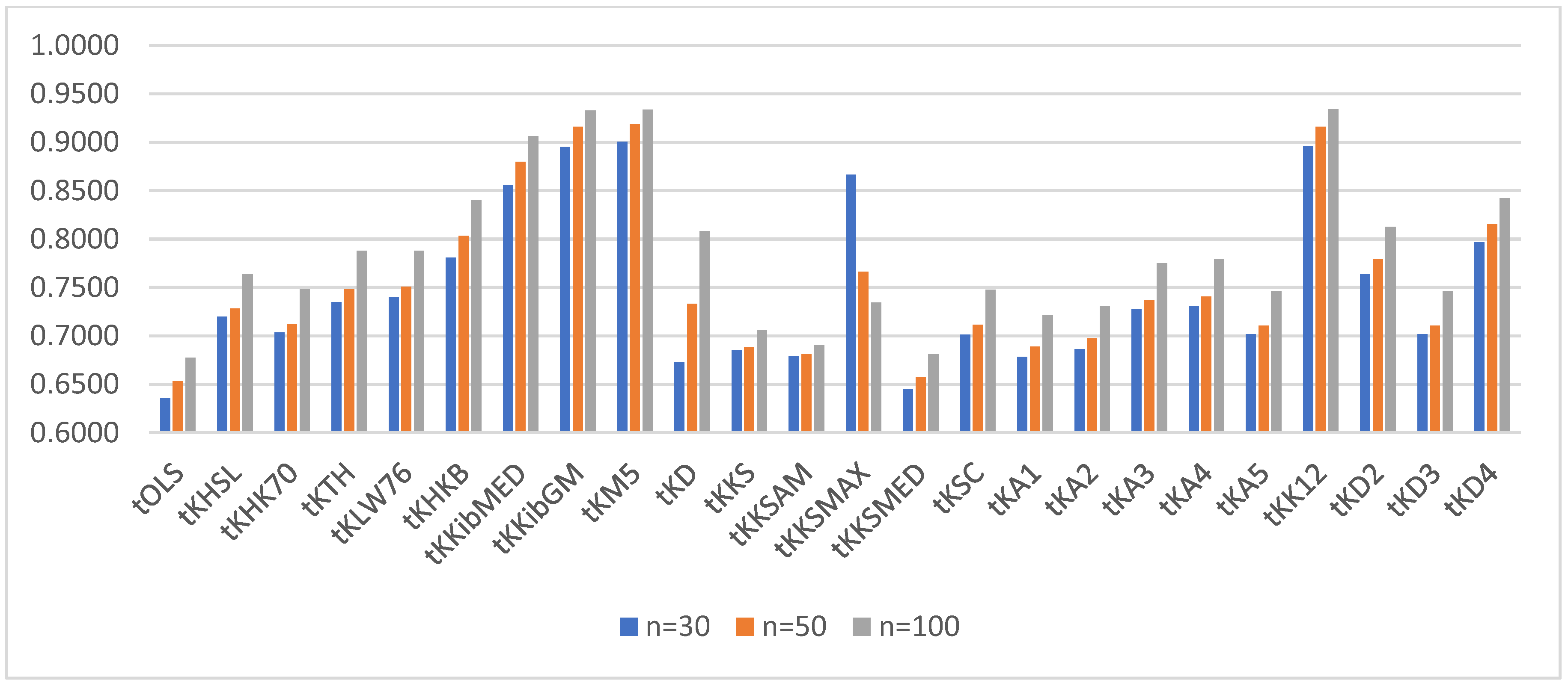
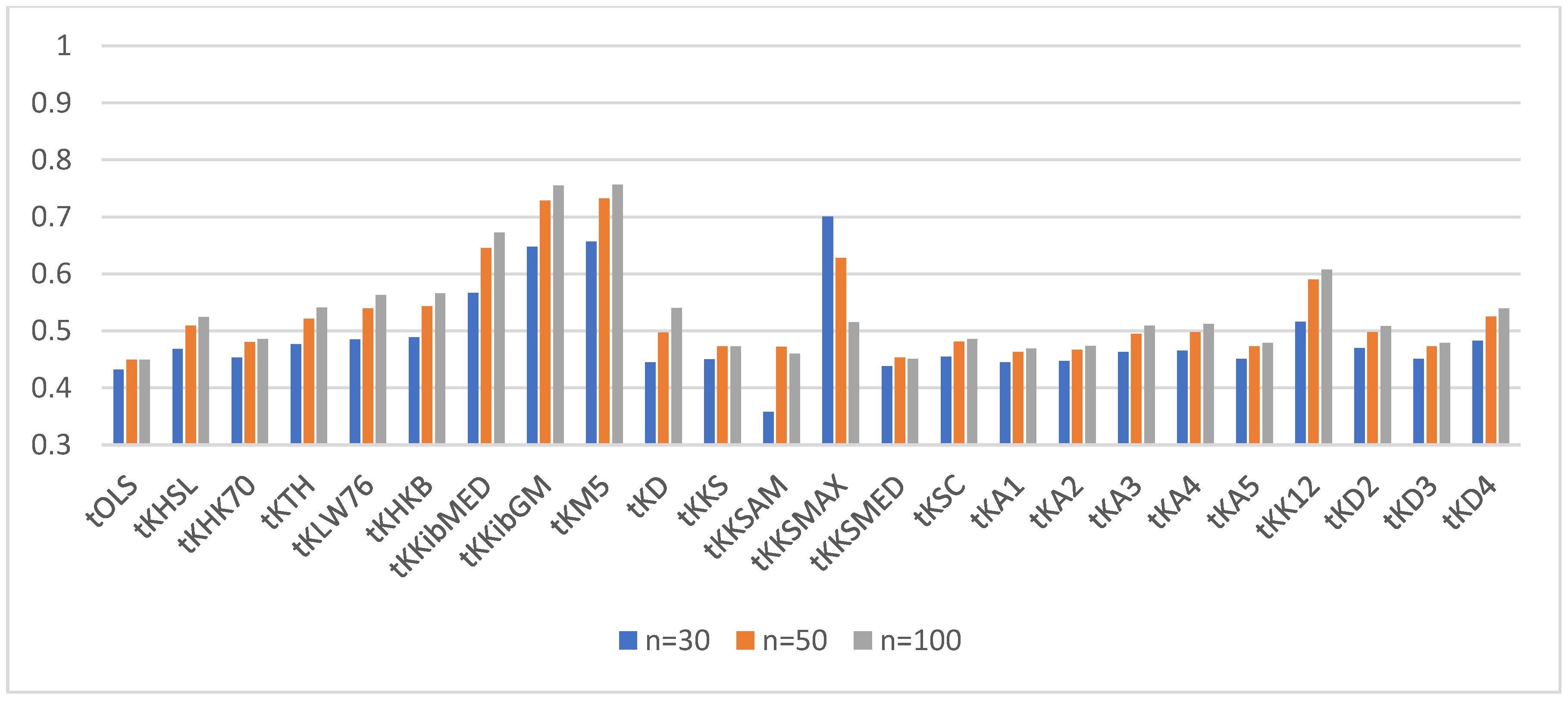
For a better visualization of the power of the ridge tests vs. the OLS test, we provided the power of the test for α = 0.05 and ρ = 0.80 and q = 4, 6, and 10 in Figure 1, Figure 2 and Figure 3, respectively.
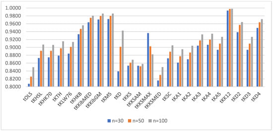
Figure 1.
Power of the test for correlation coefficient 0.80 and q = 4.
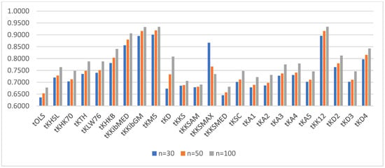
Figure 2.
Power of the test for correlation coefficient 0.80 and q = 6.
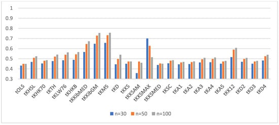
Figure 3.
Power of the test for correlation coefficient 0.80 and q = 10.
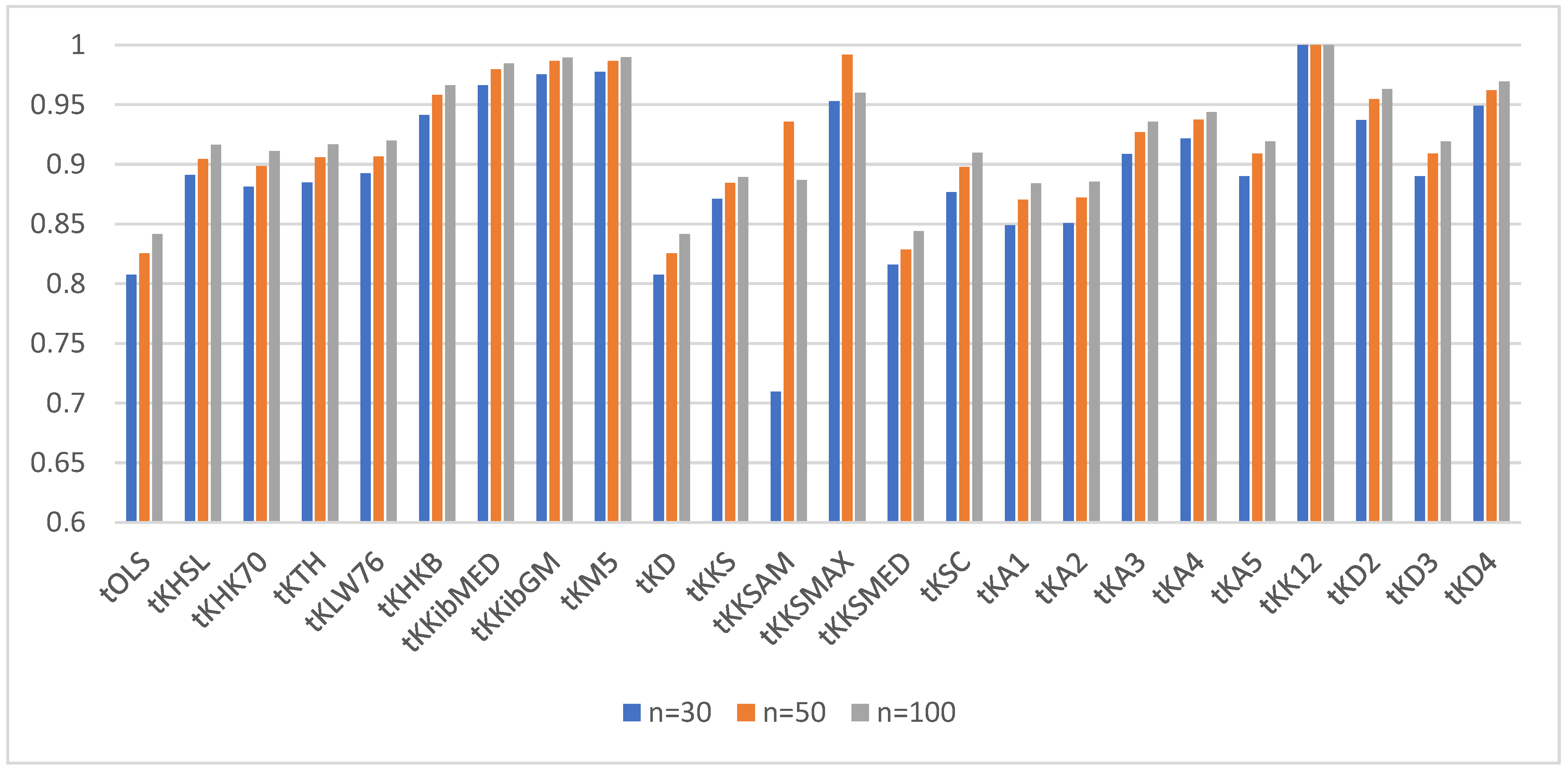
For a better visualization of the power of the ridge tests vs. the OLS test, we provided the power of the test for α = 0.05 and ρ = 0.90 and q = 4, 6, and 10 in Figure 4, Figure 5 and Figure 6, respectively.
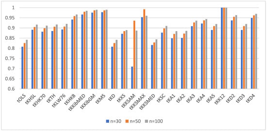
Figure 4.
Power of the test for correlation coefficient 0.95 and q = 4.
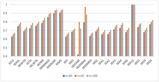
Figure 5.
Power of the test for correlation coefficient 0.95 and q = 6.

Figure 6.
Power of the test for correlation coefficient 0.95 and q = 10.
The following Table 7 provides the average gains in power for the tests with respect to the OLS test for both levels of correlations, namely 0.80 and 0.95.

Table 7.
Average gain in power over the ordinary least squares (OLS) test for α = 0.05 and q = 0.06.
Based on the above tables, we observed the following:
- (i)
- All the considered tests (with the exception of the one based on KKSAM when n = 30) achieved higher statistical power than the OLS test.
- (ii)
- Keeping the number of variables in the model fixed, if the sample size increased, the power of the tests also increased, as was expected.
- (iii)
- Keeping the sample size fixed, increasing the number of variables in the model decreased the power of the tests.
- (iv)
- Among the tests considered, the ones with the highest gain in power over the OLS test across different values of q, n, and ρ were the ones based on the following ridge estimators: KHKB, KKibMED, KKibGM, KM5, KKSMAX, KK12, and KD4. The observed gains over the OLS test were between 12% to 28% (see Table 7). Therefore, we recommend these seven tests to data analysis practitioners since they achieve the highest power among the ones considered while maintaining a 5% probability of Type I error.
4. Application Example
The following car consumption dataset available in the webpage http://data-mining-tutorials.blogspot.com/2010/05/solutions-for-multicollinearity-in.html (See Appendix A) was used to illustrate the finding of the paper.
The goal was to create a linear regression model to predict the consumption of cars from various characteristics such as: price, engine size, horsepower, and weight. There were n = 27 observations in the dataset. We made use of the mctest and the lmridge R packages in our computations. For more info on the functionality of the aforementioned packages, see Ullah, Aslam, and Altaf [36].
There was strong evidence of multicollinearity in the data, as evidenced by all of the VIFs (variance inflation factors) being greater than 10 (See Table 8 below).

Table 8.
Variance inflation factors (VIFs) of the regressors.
Also, the condition number (CN), which is defined as , was greater than 30, indicating high dependency between the explanatory variables. Since multicollinearity existed, ridge regression estimation was preferable to OLS estimation for this model. We contrasted the results of the OLS method with ridge regression using two of the ridge estimators that showed higher power, namely KKibMED and KKibGM, and the analyses are given in the following Table 9.

Table 9.
Regression analysis.
From Table 9, we observed that no variable except for weight was a significant predictor of car consumption under the OLS estimation. When ridge regression was applied, all variables (price, engine size, horsepower, and weight of the car) became significant predictors of car consumption, and the MSE [computed using Equation (5) of the coefficient vector also decreased compared to the OLS estimate, as is expected when a ridge regression approach is appropriate. Also, we could see that the sign of the coefficient of horsepower reversed from negative and not significant under the OLS estimation to positive and significant under ridge regression estimation. Change of sign in the coefficients is one of the signals that the ridge regression approach is a good fit for this particular problem according to what is explained in the foundational paper by Hoerl and Kennard [1]. Also, it makes physical sense that higher horsepower of the car leads to higher gas consumption, thus a positive sign for the coefficient would be the right choice.
5. Some Concluding Remarks
In this paper, we investigated forty different ridge regression estimators in order to find some good test statistics for testing the regression coefficients of the linear regression model in case of multicollinearity. A simulation study under different conditions was constructed to make the empirical comparison among the ridge regression estimators. We compared the performance of the test statistics based on the empirical size and the power of the test. It was observed from our simulations that the tests based on ridge estimators KHKB, KKibMED, KKibGM, KM5, KKSMAX, KK12, and KD4 were the best in terms of achieving higher power gains with respect to the OLS test while maintaining a 5% nominal size.
Our results are consistent with Kibria and Banik [29], although they did not conclude which tests were the best ones. While Gokpinar and Ebergil [28] concluded that the best tests in terms of power were the ones based on KHSL and KHKB, we found that the gains in power over the OLS test for KHSL are somewhat smaller than the gains in power for the tests based on the seven estimators we mentioned above, and therefore we did not include KHSL in our final list.
All in all, based on our simulation results, we recommend the tests based on KHKB, KKibMED, KKibGM, KM5, KKSMAX, KK12, and KD4 to statistical practitioners for the purpose of testing linear regression coefficients when multicollinearity is present.
Author Contributions
B.M.G.K. dedicates this paper to the Bangabandhu Sheikh Mujibur Rahman, the great leader and the Father of the Nation of Bangladesh. S.P.M. dedicates this paper to his parents, Consuelo de la Caridad Melo Seivane and Sergio Mariano Perez Trujillo. All authors have read and agreed to the published version of the manuscript.
Funding
This research received no external funding.
Acknowledgments
Authors are thankful to all four referees for their valuable comments and suggestions, which certainly improved the presentation and quality of the paper.
Conflicts of Interest
The authors declared no conflict of interest.
Appendix A

Table A1.
Data set.
Table A1.
Data set.
| Model | Price | Engine Size | Horsepower | Weight | Gas Consumption |
|---|---|---|---|---|---|
| Daihatsu Cuore | 11600.00 | 846.00 | 32.00 | 650.00 | 5.70 |
| Suzuki Swift 1.0 GL | 12490.00 | 993.00 | 39.00 | 790.00 | 5.80 |
| Fiat Panda Mambo L | 10450.00 | 899.00 | 29.00 | 730.00 | 6.10 |
| VW Polo 1.4 60 | 17140.00 | 1390.00 | 44.00 | 955.00 | 6.50 |
| Opel Corsa 1.2i Eco | 14825.00 | 1195.00 | 33.00 | 895.00 | 6.80 |
| Subaru Vivio 4WD | 13730.00 | 658.00 | 32.00 | 740.00 | 6.80 |
| Toyota Corolla | 19490.00 | 1331.00 | 55.00 | 1010.00 | 7.10 |
| Opel Astra 1.6i 16V | 25000.00 | 1597.00 | 74.00 | 1080.00 | 7.40 |
| Peugeot 306 XS 108 | 22350.00 | 1761.00 | 74.00 | 1100.00 | 9.00 |
| Renault Safrane 2.2 | 36600.00 | 2165.00 | 101.00 | 1500.00 | 11.70 |
| Seat Ibiza 2.0 GTI | 22500.00 | 1983.00 | 85.00 | 1075.00 | 9.50 |
| VW Golt 2.0 GTI | 31580.00 | 1984.00 | 85.00 | 1155.00 | 9.50 |
| Citroen ZX Volcane | 28750.00 | 1998.00 | 89.00 | 1140.00 | 8.80 |
| Fiat Tempra 1.6 Lib | 22600.00 | 1580.00 | 65.00 | 1080.00 | 9.30 |
| Fort Escort 1.4i PT | 20300.00 | 1390.00 | 54.00 | 1110.00 | 8.60 |
| Honda Civic Joker 1 | 19900.00 | 1396.00 | 66.00 | 1140.00 | 7.70 |
| Volvo 850 2.5 | 39800.00 | 2435.00 | 106.00 | 1370.00 | 10.80 |
| Ford Fiesta 1.2 Zet | 19740.00 | 1242.00 | 55.00 | 940.00 | 6.60 |
| Hyundai Sonata 3000 | 38990.00 | 2972.00 | 107.00 | 1400.00 | 11.70 |
| Lancia K 3.0 LS | 50800.00 | 2958.00 | 150.00 | 1550.00 | 11.90 |
| Mazda Hachtback V | 36200.00 | 2497.00 | 122.00 | 1330.00 | 10.80 |
| Opel Omega 2.5i V6 | 47700.00 | 2496.00 | 125.00 | 1670.00 | 11.30 |
| Peugeot 806 2.0 | 36950.00 | 1998.00 | 89.00 | 1560.00 | 10.80 |
| Nissan Primera 2.0 | 26950.00 | 1997.00 | 92.00 | 1240.00 | 9.20 |
| Seat Alhambra 2.0 | 36400.00 | 1984.00 | 85.00 | 1635.00 | 11.60 |
| Toyota Previa salon | 50900.00 | 2438.00 | 97.00 | 1800.00 | 12.80 |
| Volvo 960 Kombi aut | 49300.00 | 2473.00 | 125.00 | 1570.00 | 12.70 |
References
- Hoerl, A.E.; Kennard, R.W. Ridge regression: Biased estimation for non-orthogonal problems. Technometrics 1970, 12, 55–67. [Google Scholar] [CrossRef]
- Hoerl, A.E.; Kennard, R.W.; Baldwin, K.F. Ridge regression: Some simulation. Commun. Stat. Theory Methods 1975, 4, 105–123. [Google Scholar] [CrossRef]
- Lawless, J.F.; Wang, P. A simulation study of ridge and other regression estimators. Commun. Stat. Simul. Comput. 1976, 5, 307–323. [Google Scholar]
- Gibbons, D.G. A simulation study of some ridge estimators. J. Am. Stat. Assoc. 1981, 76, 131–139. [Google Scholar] [CrossRef]
- Nomura, M. On the almost unbiased ridge regression estimation. Commun. Stat. Simul. Comput. 1988, 17, 729–743. [Google Scholar] [CrossRef]
- Kibria, B.M.G. Performance of some new ridge regression estimators. Commun. Stat. Simul. Comput. 2003, 32, 419–435. [Google Scholar] [CrossRef]
- Khalaf, G. A Proposed Ridge Parameter to Improve the Least Square Estimator. J. Mod. Appl. Stat. Methods 2012, 11, 443–449. [Google Scholar] [CrossRef]
- Khalaf, G.; Shukur, G. Choosing ridge parameters for regression problems. Commun. Stat. Theory Methods 2005, 34, 1177–1182. [Google Scholar] [CrossRef]
- Alkhamisi, M.; Shukur, G. Developing ridge parameters for SUR model. Commun. Stat. Theory Methods 2008, 37, 544–564. [Google Scholar] [CrossRef]
- Muniz, G.; Kibria, B.M.G. On some ridge regression estimators: An empirical comparison. Commun. Stat. Simul. Comput. 2009, 38, 621–630. [Google Scholar] [CrossRef]
- Feras, M.B.; Gore, S.D. Ridge regression estimator: Combining unbiased and ordinary ridge regression methods of estimation. Surv. Math. Appl. 2009, 4, 99–109. [Google Scholar]
- Gruber, M.H.J. Improving Efficiency by Shrinkage the James-Stein and Ridge Regression Stimators; Marcel Dekker: New York, NY, USA, 1998. [Google Scholar]
- Muniz, G.; Kibria, B.M.G.; Mansson, K.; Shukur, G. On developing ridge regression parameters: A graphical investigation. Stat. Oper. Res. Trans. 2012, 36, 115–138. [Google Scholar]
- Mansson, K.; Shukur, G.; Kibria, B.M.G. On some ridge regression estimators: A Monte Carlo simulation study under different error variances. J. Stat. 2010, 17, 1–22. [Google Scholar]
- Hefnawy, E.A.; Farag, A. A combined nonlinear programming model and Kibria method for choosing ridge parameter regression. Commun. Stat. Simul. Comput. 2013. [Google Scholar] [CrossRef]
- Roozbeh, M.; Arashi, M. Feasible ridge estimator in partially linear models. J. Multivar. Anal. 2013, 116, 35–44. [Google Scholar] [CrossRef]
- Arashi, M.; Valizadeh, T. Performance of Kibria’s methods in partial linear ridge regression model. Stat. Pap. 2014, 56, 231–246. [Google Scholar] [CrossRef]
- Aslam, M. Performance of Kibria’s method for the heteroscedastic ridge regression model: Some Monte Carlo evidence. Commun. Stat. Simul. Comput. 2014, 43, 673–686. [Google Scholar] [CrossRef]
- Asar, Y.; Karaibrahimoğlu, G.A. Modified ridge regression parameters: A comparative Monte Carlo study. Hacet. J. Math. Stat. 2014, 43, 827–841. [Google Scholar]
- Saleh, A.K.M.E.; Arashi, M.; Tabatabaey, S.M.M. Statistical Inference for Models with Multivariate T-Distributed Errors; John Wiley: Hoboken, NJ, USA, 2014. [Google Scholar]
- Asar, Y.; Erişoğlu, M. Influence diagnostics in two-parameter ridge regression. J. Data Sci. 2016, 14, 33–52. [Google Scholar]
- Goktas, A.; Sevnic, V. Two new ridge parameters and a guide for selecting an appropriate ridge parameter in linear regression. Gazi Univ. J. Sci. 2016, 29, 201–211. [Google Scholar]
- Fallah, R.; Arashi, M.; Tabatabasy, S.M.M. On the ridge regression estimator with sub-space restriction. Commun. Stat. Theory Methods 2017, 46, 11854–11865. [Google Scholar] [CrossRef]
- Norouzirad, M.; Arashi, M. Preliminary test and stein-type shrinkage ridge estimators in robust regression. Stat. Pap. 2019, 60, 1849–1882. [Google Scholar] [CrossRef]
- Saleh, A.K.M.E.; Arashi, M.; Kibria, B.M.G. Theory of Ridge Regression Estimation with Applications; John Woley: Hoboken, NJ, USA, 2019. [Google Scholar]
- Halawa, A.M.; Bassiouni, M.Y. Tests of regression coefficients under ridge regression models. J. Stat. Simul. Comput. 2000, 65, 341–356. [Google Scholar] [CrossRef]
- Cule, E.; Vineis, P.; De Iorio, M. Significance testing in ridge regression for genetic data. BMC Bioinform. 2011, 12, 372. [Google Scholar] [CrossRef] [PubMed]
- Gökpınar, E.; Ebegil, M. A study on tests of hypothesis based on ridge estimator. Gazi Univ. J. Sci. 2016, 29, 769–781. [Google Scholar]
- Kibria, B.M.G.; Banik, S. A simulation study on the size and power properties of some ridge regression tests. Appl. Appl. Math. Int. J. (AAM) 2019, 14, 741–761. [Google Scholar]
- Hocking, R.R.; Speed, F.M.; Lynn, M.J. A class of biased estimators in linear regression. Technometrics 1976, 18, 425–437. [Google Scholar] [CrossRef]
- Thisted, R.A. Ridge Regression, Minimax Estimation and Empirical Bayes Methods; Technical Report 28; Division of Biostatistics, Stanford University: Stanford, CA, USA, 1976. [Google Scholar]
- Venables, W.N.; Ripley, B.D. Modern Applied Statistics with S, 4th ed.; Springer: New York, NY, USA, 2002; ISBN 0-387-95457-0. [Google Scholar]
- Dorugade, A.; Kashid, D. Alternative Method for Choosing Ridge Parameter for Regression. Appl. Math. Sci. 2010, 4, 447–456. [Google Scholar]
- Schaefer, R.; Roi, L.; Wolfe, R. A ridge logistic estimator. Commun. Stat. Theory Methods 1984, 13, 99–113. [Google Scholar] [CrossRef]
- Dorugade, A. New Ridge Parameters for Ridge Regression. J. Assoc. Arab Univ. Basic Appl. Sci. 2014, 15, 94–99. [Google Scholar] [CrossRef]
- Ullah, M.I.; Aslam, M.; Altaf, S. lmridge: A comprehensive R package for ridge regression. R J. 2018, 10, 326–346. [Google Scholar] [CrossRef]
© 2020 by the authors. Licensee MDPI, Basel, Switzerland. This article is an open access article distributed under the terms and conditions of the Creative Commons Attribution (CC BY) license (http://creativecommons.org/licenses/by/4.0/).

