A Bayesian Approach to Predict the Number of Goals in Hockey

Abstract

In this paper, we use a Bayesian methodology to analyze the outcome of a hockey game using different sources of information, such as points in previous games, home advantage, and specialists’ opinions. Two different models to predict the number of goals are considered, taking into account that it is the nature of hockey that goals are infrequent and rarely exceed six per team per game. A Bayesian predictive density to predict the number of the goals using each model will be used and the possible winner of the game will be predicted. The corresponding prediction error for each model will be addressed.

1. Introduction

Finding ways of predicting the outcome in different sport games from past and current data is an attractive problem for different people, ranging from the sports teams’ coaches to gambling agencies to fans of that sport. There is no doubt that statistical tools are needed to construct an effective and accurate model to predict the outcome of sporting events. In the last decades, predicting match results has attracted much attention from researchers using new methods of statistics, data mining and machine learning, especially in popular sports such as football, basketball, baseball and soccer.

Ice hockey is a popular sport especially in the US and Canada for which there exists a rich dataset available at www.nhl.com. Several publications have appeared in recent years documenting different statistical analysis of the hockey data. Gramacy et al. [1] studied individual contributions of team members using regularized logistic regression. Sadeghkhani and Ahmed [2] estimated the density of scoring time in a hockey game using prior information such as a team’s ranking in the previous season and experts’ opinions. Suzuki et al. [3] proposed a Bayesian approach in predicting the match outcomes in the 2006 World Cup.

However, to the authors’ best knowledge, very few publications currently available in the literature address the issue of Bayesian density estimation of number of the goals. This paper proposes a unique method to estimate the density of number of the goals. We also consider the points in the previous games, away and home factors, and specialists’ opinions to improve our predictions.

The remainder of the paper is organized as follows: In Section 2, we provide definitions and preliminary remarks about two assumptions to model the number of goals in a hockey game. Section 3 discusses how to find Bayesian predictive density estimators for each model. Section 4 addresses how one can enter other factors such as home bonus, away malus, experts’ opinions in detail. In Section 5, we study an application of the proposed methods in predicting the number of goals as well as the result of the game. Finally, we make some concluding remarks in Section 6.

2. Problem Set-Up and Different Models

Poisson distribution has been used in the context of count data, but the fact that the dispersion index (the ratio of variance to mean) equals one is a big concern in practice. Conway and Maxwell [4] introduced the Conway–Maxwell–Poisson (COM-P) distribution, which, similar to the Poisson distribution, belongs to the exponential family of distributions and, therefore, the Bayesian analysis (because of the conjugate prior) of number of events becomes more computationally tractable.

Kadane et al. [5] studied a necessary and sufficient condition on the hyperparameters of the conjugate family for the prior to be proper and discussed methods of sampling from the conjugate distribution.

The COM-P distribution processes an extra parameter and was originally developed as a solution of handling a queuing system with state-dependant arrivals. It has has been used widely in the models that that have over-dispersion or under-dispersion, i.e., the mean is smaller or larger than variance, respectively. For more information, see Shmueli et al. [6].

A random variable (rv for short) has the $COM-P(\lambda ,r)$ distribution if it has the probability mass function (pmf) in the form of

$$P(X=x\mid \lambda ,r)=\frac{1}{Z(\lambda ,r)}\frac{{\lambda }^x}{{(x!)}^r},x=0,1,\dots ,r>0,\lambda >0,$$

(1)

where $Z(\lambda ,r)={\sum }_{j=0}^{\infty }\frac{{\lambda }^j}{{(j!)}^r}$ is the normalizing constant. It is easy to see the Poisson distribution, $Po\left(\lambda \right)$, obtained when $r=1$. Furthermore, the density in (1) belongs to exponential family and values of $r>1$ and $r<1$ are equivalent to under- and over- dispersion each. When $\lambda \in (0,1)$, tending $r\to inf$ gives Bernoulli with parameter $\lambda$ while the geometric distribution corresponds to limiting $r\to 0$ with pmf of $P(X=x\mid \lambda )={\lambda }^x(1-\lambda )$, for $x=0,1,\dots$.

Imoto [7] generalized the COM-P to a distribution which has a larger tail and embraces the negative binomial distribution and applicable to the excess zeros model as well.

An rv X is said to have a generalized COM-P (GCOM-P) with three parameters $\lambda >0$, $r>0$ and $\nu >0$, if

$$P(X=x\mid \lambda ,r,\nu )=\frac{{(\Gamma (x+\nu ))}^r{\lambda }^x}{x!C(\lambda ,r,\nu )},x=0,1,\dots ,$$

(2)

where $C(\lambda ,r,\nu )={\sum }_{j=0}^{\infty }\frac{{(\Gamma (j+\nu ))}^r{\lambda }^j}{j!}$ is the normalizing constant. When $r<1$, $\nu >0$ and $\lambda >0$ or $r=1$, $\nu >0$ and $\lambda \in (0,1)$, $C(\lambda ,r,\nu )$ converge. This distribution reduces to a COM-P distribution with parameter $\lambda$ and $1-r$ when $\nu \to 1$ and to a negative binomial when $r=1$.

3. Bayesian Prior and Posterior Predictive Density Estimations

As can be seen in the literature, gamma distribution is being used as conjugate prior for a Poisson distribution. Suppose $X\sim Po(\lambda$), choosing $\lambda \mid \alpha ,\beta \sim Gam(\alpha ,\beta )$ with the pdf $\frac{1}{\Gamma \left(\alpha \right){\beta }^{\alpha }}{\lambda }^{\alpha -1}{e}^{-\lambda /\beta }$ results in the posterior density $\lambda \mid x,\alpha ,\beta \sim Gam(x+\alpha ,\frac{1}{1+1/\beta })$. The marginal distribution of X, known as a prior predictive density estimator, and posterior predictive density estimator are negative binomial distribution. Rv $X\sim NB(r,p)$ has the pmf $P(X=k)=\left(\genfrac{}{}{0pt}{}{k}{k+r-1}\right){(1-p)}^r{p}^k$, $k=0,1,\dots$.

Lemma 1.

If $X\sim Po\left(\lambda \right)$ and $\lambda \mid \alpha ,\beta \sim Gam(\alpha ,\beta )$, the prior predictive density $P(X=x\mid \alpha ,\beta )$ is given by

$$NB\left(\alpha ,\frac{1}{1+1/\beta }\right),$$

(3)

while the posterior predictive density of future rv. Y, $P(Y=y\mid X_1=x_1,\cdots ,X_n=x_n,\alpha ,\beta )$ is given by

$$NB\left({\displaystyle \sum _1^n}{x}_i+\alpha ,\frac{1}{1+n+1/\beta }\right).$$

(4)

Proof. 

The prior predictive in (3) is the marginal distribution of X and can be found as follows:

$$\begin{array}{cc}\hfill P(X=x\mid \alpha ,\beta )& ={\int }_0^{\infty }P(X=x\mid \lambda )\pi (\lambda \mid \alpha ,\beta )d\lambda \hfill \\ & =\frac{1}{x!\Gamma \left(\alpha \right)}\frac{1}{{\beta }^{\alpha }}{\int }_0^{\infty }{\lambda }^{\alpha +x-1}{e}^{-\lambda (1+1/\beta )}d\lambda \hfill \\ & =\frac{1}{\Gamma (x+1)\Gamma \left(\alpha \right)}\frac{1}{{\beta }^{\alpha }}\Gamma (\alpha +x){\left(\frac{\beta }{1+\beta }\right)}^{\alpha +x}\hfill \\ & =\left(\genfrac{}{}{0pt}{}{\alpha +x-1}{x}\right){\left(\frac{1}{1+\beta }\right)}^{\alpha }{\left(1-\frac{1}{1+1/\beta }\right)}^x.\hfill \end{array}$$

Equation (4) can be obtained similarly from

$$p(y\mid \mathbf{x})={\int }_0^{\infty }P(y\mid \theta )\pi (\theta \mid \mathbf{x})d\theta ,$$

and the posterior density of $\lambda$ based on $\mathbf{x}=(x_1,\cdots ,x_n)$, is $Gam(x+\alpha ,\frac{1}{n+1/\beta })$. □

In the COM-P model, Equation (1), Kadane et al. [5] used the extended bivariate gamma distribution denoted by $EBG(a,b,c)$, and given by

$$\pi (\lambda ,r\mid a,b,c)=\kappa (a,b,c){\lambda }^{a-1}{e}^{-rb}{Z}^{-c}(\lambda ,r),$$

(5)

where the normalization constant in (5), is given by

$${\kappa }^{-1}(a,b,c)={\int }_0^{\infty }{\int }_0^{ı}{\lambda }^{a-1}{e}^{-rb}{Z}^{-c}(\lambda ,r)d\lambda dr,$$

and $a>0$, $b>0$ and $c>0$ needs to satisfy the following condition so that ${\kappa }^{-1}(a,b,c)$ becomes finite:

$$\frac{b}{c}>log(\lfloor \frac{a}{c}\rfloor !)+(\frac{a}{c}-\lfloor \frac{a}{c}\rfloor )log(\lfloor \frac{a}{c}\rfloor +1).$$

Next lemma, similarly to Lemma 1, provides the predictive distributions.

Lemma 2.

If $X_i\sim COM-P(\lambda ,r);$$i=1,\cdots ,n$, as in (1), for $i=1,\dots ,n$, and $\pi (\lambda ,r\mid a,b,c)$ presented in (5), then:

• the posterior has the same distribution to (5) with $a^{*}=a+{\sum }_1^n{x}_i$, $b^{*}=b+{\sum }_1^{n}log(x_i!)$, and $c^{*}=c+n$.
• the prior predictive density (marginal density of X) is given by

  $$P(X=x\mid a,b,c)=\frac{\kappa (a,b,c)}{\kappa (a+x,b+log(x!),c+1)}.$$

  (6)
• the posterior predictive density of future rv Y, $P(Y=y\mid X_1=x_1,\dots ,X_n=x_n,a,b,c)$ for $y=0,1,\dots$ is given by

  $$\frac{\kappa (a^{*},b^{*},c^{*})}{\kappa (a^{*}+y,b^{*}+log(y!),c^{*}+1)}.$$

  (7)

Proof. 

The proof is straightforward and analogous to the proof of Lemma 1 and has therefore been omitted. □

4. Modelling Number of Goals Using Prior Elicitation Method

In this section, we make two different assumptions: (I) let us assume the number of goals scored by each team is a Poisson rv and (II) it has COM-P. In addition, suppose that A is a team playing home and B is a team playing away and hence, $X_{AB}$ is the number of goals scored by team A to team B and $X_{BA}$, vice-versa.

4.1. Assumption I: $Po$ Distribution for Modelling Number of Goals

Assume that $X_{AB}$ and $X_{BA}$, are independently distributed as follows:

$$\begin{array}{c}\hfill X_{AB}\mid {\lambda }_{AB}\sim Po\left({\lambda }_{AB}\right),X_{BA}\mid {\lambda }_{BA}\sim Po\left({\lambda }_{BA}\right),\end{array}$$

(8)

where ${\lambda }_{AB}$ can be interpreted as the mean number of goals team A scores against team B and ${\lambda }_{BA}$ is the number of goals team B scores against team A in a future game. As discussed earlier, one can use conjugate prior $\pi \left({\lambda }_{AB}\right)$ (for home) as a $Gam(\alpha ,\beta )$, where the jeffreys non–informative prior ${\pi }_0\left(\lambda \right)\propto {\lambda }_{AB}^{-\frac{1}{2}}$ is its special case. Here, we are interested in employing experts’ opinions about the upcoming match’s score. This is called prior elicitation and can be determined by ${\pi }_e(·)$:

$$\begin{array}{c}\hfill {\pi }_e\left({\lambda }_{AB}\right)\propto \pi \left({\lambda }_A\right){\left\{{\displaystyle \prod _{i=1}^s}{e}^{-{\lambda }_A}{{\lambda }_{AB}}^{x_{iAB}^{\prime }}\right\}}^d\equiv Gam(\alpha +d{\displaystyle \sum _{i=1}^s}{x}_{iAB}^{\prime },\frac{1}{\beta }+sd),\end{array}$$

(9)

where $x_{iAB}^{\prime }$, $i=1,2,\dots ,s$, is the i-th expert’s opinion about number of goals that home team A will score against away team B in the future game. Choosing $d=0$ returns the $\pi (·)$ as a prior and ignores the specialists’ opinion factor. Analogously, we can set prior of ${\lambda }_{BA}$ in the same manner.

We have used the specialists to improve our beliefs about ${\lambda }_{AB}$ (or ${\lambda }_{BA}$), but we can also benefit from other sources of information, such as previous data. Since usually (not necessarily) the number of goals is larger when team plays home and smaller when team plays away, we can use the model home-bonus factor h, and away or visiting-malus factor v.

$$\begin{array}{cc}\hfill h& =\frac{\mathrm{Mean}\mathrm{of}\mathrm{goals}\mathrm{scored}\mathrm{by}\mathrm{team}A\mathrm{at}\mathrm{home}\mathrm{versus}\mathrm{team}B\mathrm{in}\mathrm{previous}\mathrm{matches}}{\mathrm{Mean}\mathrm{of}\mathrm{goals}\mathrm{by}\mathrm{all}\mathrm{the}\mathrm{team}\mathrm{in}\mathrm{hosting}\mathrm{their}\mathrm{opponents}},\hfill \\ \hfill v& =\frac{\mathrm{Mean}\mathrm{of}\mathrm{goals}\mathrm{scored}\mathrm{by}\mathrm{team}B\mathrm{away}\mathrm{versus}\mathrm{team}A\mathrm{in}\mathrm{previous}\mathrm{matches}}{\mathrm{Mean}\mathrm{of}\mathrm{goals}\mathrm{by}\mathrm{all}\mathrm{the}\mathrm{team}\mathrm{on}\mathrm{the}\mathrm{way}\mathrm{with}\mathrm{their}\mathrm{opponents}}.\hfill \end{array}$$

Alternatively, one can consider the teams’ points as well. The mean of number of goals A scores versus team B is directly related to h and points obtained by team A, namely $Q_A$ (in the previous games or last season), and has an indirect relationship with a and points obtained by team B, $Q_B$. Consequently, we can update prior density in (9) (for both ${\lambda }_{AB}$ and ${\lambda }_{BA}$ ) as follows:

$$\begin{array}{cc}\hfill {\lambda }_{AB}& \sim Gam\left(\alpha +d{\displaystyle \sum _{i=1}^s}{x}_{iAB}^{\prime },\frac{Q_A}{Q_B}\frac{h}{v}\left(\frac{1}{\beta }+sd\right)\right),\hfill \end{array}$$

(10)

$$\begin{array}{cc}\hfill {\lambda }_{BA}& \sim Gam\left(\alpha +d{\displaystyle \sum _{i=1}^s}{x}_{iBA}^{\prime },\frac{Q_B}{Q_A}\frac{v}{h}\left(\frac{1}{\beta }+sd\right)\right).\hfill \end{array}$$

(11)

Making use of Equations (10) and (11), along with Lemma 1, gives the prior and posterior predictive density estimators for the number of goals team A scores to team B, which are, respectively, given by

$$\begin{array}{cc}\hfill X_{AB}& \sim NB\left(d{\displaystyle \sum _{i=1}^s}{x}_{iAB}^{\prime }+\alpha ,\frac{1}{1+{\left(\frac{Q_A}{Q_B}\frac{h}{v}\left(\frac{1}{\beta }+sd\right)\right)}^{-1}}\right)\hfill \end{array}$$

(12)

and

$$\begin{array}{cc}\hfill X_{AB}& \sim NB\left({\displaystyle \sum _{i=1}^{n_{AB}}}{x}_{iA}+d{\displaystyle \sum _{i=1}^s}{x}_{iAB}^{\prime }+\alpha ,\frac{1}{1+n+{\left(\frac{Q_A}{{\overline{Q}}_E}\frac{h}{v}\left(\frac{1}{\beta }+sd\right)\right)}^{-1}}\right),\hfill \end{array}$$

(13)

where $x_{iA}$ is the number of goals team A has scored in the previous season (or prior to the upcoming game) when played at home versus opponents and ${\overline{Q}}_E={\sum }_1^{n_{AB}}{Q}_{E_i}/n_{AB}$ and $Q_{E_i}$’s are (all) opponents’ points in previous season (or prior to the upcoming game) who faces team A and $n_{AB}$ is the number of games team A host team B. Similarly, for the number of goals, team B scores in the home of team A, we have

$$\begin{array}{cc}\hfill X_{BA}& \sim NB\left(d{\displaystyle \sum _{i=1}^s}{x}_{iBA}^{\prime }+\alpha ,\frac{1}{1+{\left(\frac{Q_B}{Q_A}\frac{v}{h}\left(\frac{1}{\beta }+sd\right)\right)}^{-1}}\right),\hfill \end{array}$$

(14)

$$\begin{array}{cc}\hfill X_{BA}& \sim NB\left({\displaystyle \sum _{i=1}^{n_{BA}}}{x}_{iB}+d{\displaystyle \sum _{i=1}^s}{x}_{iBA}^{\prime }+\alpha ,\frac{1}{1+n+{\left(\frac{Q_B}{{\overline{Q}}_D}\frac{h}{v}\left(\frac{1}{\beta }+sd\right)\right)}^{-1}}\right),\hfill \end{array}$$

(15)

where $x_{iB}$ is the number of goals team B has scored in the previous season (or up to upcoming game) when played on the way versus opponents and ${\overline{Q}}_D={\sum }_1^{n_{BA}}{Q}_{D_i}/n_{BA}$ and $Q_{D_i}$’s are (all) opponents’ points in previous season (or prior to the upcoming match) who hosted team B.

4.2. Assumption II: $COM-P$ Model of Number of Goals

A question that may arise is, “What if the distributions of the number of goals do not obey a Poisson distribution?” In this assumption we contemplate the $COM-P(\lambda ,r)$ distribution given in (1) as a distribution of the number of goals. Therefore, $X_{AB}$ and $X_{BA}$ are independently distributed as follows:

$$\begin{array}{c}\hfill X_{AB}\mid {\lambda }_{AB},r_{AB}\sim COM-P\left({\lambda }_{AB},r_{AB}\right),X_{BA}\mid {\lambda }_{BA},r_{BA}\sim COM-P\left({\lambda }_{BA},r_{BA}\right).\end{array}$$

(16)

We use $EBG(a,b,c)$ in (5) as a conjugate prior. Note that for instance, the conditional distribution $\pi ({\lambda }_{AB}\mid r_{AB}=1)$ is $Gam(a,c)$ and $\pi ({\lambda }_{AB}\mid r_{AB}=0)$ is $Bet(a,c+1)$, where Bet is a beta distribution. Similar to assumption (I), the corresponding prior elicitation can be defined as follows:

$$\begin{array}{c}\hfill {\pi }_e({\lambda }_{AB},r_{AB})\propto \pi ({\lambda }_{AB},r_{AB}){\left\{{\displaystyle \prod _{i=1}^s}{e}^{-r_{AB}log(x_{iAB}^{\prime }!)}{{\lambda }_{AB}}^{x_{iAB}^{\prime }}Z{({\lambda }_{AB},r_{AB})}^{-1}\right\}}^d,\end{array}$$

(17)

which is the $EBG(a_{AB}^{\prime },b_{AB}^{\prime },c_{AB}^{\prime })$, with

$$\begin{array}{cc}\hfill a_{AB}^{\prime }& =d{\displaystyle \sum _1^s}{x}_{iAB}^{\prime }+{\displaystyle \sum _1^{n_{AB}}}{x}_{iAB}+a,\hfill \\ \hfill b_{AB}^{\prime }& =d{\displaystyle \sum _1^s}log(x_{iAB}^{\prime }!)+{\displaystyle \sum _1^{n_{AB}}}log(x_{iAB}!)+b,\hfill \\ \hfill c_{AB}^{\prime }& =c+n_{AB}+sd,\hfill \end{array}$$

where $n_{AB}$ is number of goals scored in a game where team A is at home, hosting teams similar to team B when they were on the road. $x_{iAB}^{\prime }$, $i=1,2,\dots ,s$, $x_{iAB}$, $i=1,2,\dots ,n_{AB}$ are as defined in assumption (I). This can be done similarly to obtain ${\pi }_e({\lambda }_{BA},r_{BA})$, $a_{BA}^{\prime }=d{\sum }_1^s{x}_{iBA}^{\prime }+{\sum }_1^{n_{BA}}{x}_{iBA}+a$, $b_{BA}^{\prime }=d{\sum }_1^{s}log(x_{iBA}^{\prime }!)+{\sum }_1^{n_{BA}}log(x_{iBA}!)+b$, and $c_{BA}^{\prime }=c+n_{BA}+sd$, correspondingly.

Finally, we can pose the other additional information home–bonus factor h, away–malus factor v, points $Q_A$ and, $Q_B$ into our prior yielding the joint distribution $({\lambda }_{AB},r_{AB})$ and $({\lambda }_{BA},r_{BA})$ obtained from

$$\begin{array}{cc}\hfill & EBG\left(a_{AB}^{\prime },b_{AB}^{\prime },\frac{Q_A}{Q_B}\frac{h}{v}{c}_{AB}^{\prime }\right),\hfill \end{array}$$

(18)

$$\begin{array}{c}EBG\left(a_{BA}^{\prime },b_{BA}^{\prime },\frac{Q_B}{Q_A}\frac{v}{h}{c}_{BA}^{\prime }\right).\hfill \end{array}$$

(19)

Using (18) and (19), along with Lemma 2, result in obtaining the prior predictive density estimation of the number of goals team A scores against team B as follows:

$$\begin{array}{c}\hfill \frac{\kappa \left(d{\sum }_1^s{x}_{iAB}^{\prime }+a,d{\sum }_1^{s}log(x_{iAB}^{\prime }!)+b,\frac{Q_A}{Q_B}\frac{h}{v}(c+d)\right)}{\kappa \left(d{\sum }_1^s{x}_{iAB}^{\prime }+x_{AB}+a,d{\sum }_1^{s}log(x_{iAB}^{\prime }!)+log(x_{AB}!)+b,\frac{Q_A}{Q_B}\frac{h}{v}(c+d)+1\right)}.\end{array}$$

(20)

Furthermore, the posterior predictive density of the number of goals team A scores against team B is as follows:

$$\begin{array}{c}\hfill \frac{\kappa \left(a_{AB}^{\prime },b_{AB}^{\prime },\frac{Q_A}{Q_B}\frac{h}{v}{c}^{\prime }\right)}{\kappa \left(a_{AB}^{\prime }+x,b_{AB}^{\prime }+log(x!),\frac{Q_A}{Q_B}\frac{h}{v}{c}_{AB}^{\prime }+1\right)}.\end{array}$$

(21)

Equations (20) and (21) hold for number of goals teams B scores versus team A by replacing $a_{AB}^{\prime }$, $b_{AB}^{\prime }$, with $a_{BA}^{\prime }$, $b_{BA}^{\prime }$, respectively.

5. Example of Predicting the Scores and Results

This section addresses prediction results based on our models, as attained in the previous section. For a given match team where A hosts team B, outcomes of that match under the format win, draw and loss can be predicted via the number of goals scored by the two teams, A and B. Let the probabilities associated with win, draw and loss of team A from the predictive distributions versus team B, denoted by ${\pi }_w$, ${\pi }_d$ and ${\pi }_l$. So we can write ${\pi }_w=P(X_{AB}>X_{BA})={\sum }_{i=1}^{\infty }{\sum }_{j=0}^{i-1}P(X_{AB}=i)P(X_{BA}=j)$, ${\pi }_d=P(X_{AB}=X_{BA})={\sum }_{i=0}^{\infty }P(X_{AB}=i)P(X_{BA}=i)$, and ${\pi }_l=1-{\pi }_w-{\pi }_d$.

Let us suppose that we are interested in predicting the match outcome of A: Edmonton Oilers (home) vs B: Arizona Coyotes (away). Data for the season 2017/18 plus current season 2018/19 until the date of writing this manuscript on 29 January 2019 available at nhl.com has been used. In order to use experts’ opinions, we have asked 5 specialists to give their opinion about the upcoming match result, $x_{iAB}^{\prime }$ and $x_{iBA}^{\prime }$ as follows:

$x_{iAB}^{\prime }$	5	1	6	1	4
$x_{iBA}^{\prime }$	2	3	3	2	1

Moreover, the number of goals the Edmonton Oilers scored versus teams which had similar performance to the Arizona Coyotes when playing as a visitor, points per game, and the number of goals Arizona scored versus the teams had similar performance to Edmonton when playing at home (we asked specialists about those teams) are given in

Table 1. (Left) Table of the number of goals the Edmonton Oilers scored in the $2018/19$ season (up to 29 January) versus the Arizona Coyotes as well as teams with the similar abilities to the Arizona Coyotes, playing away. (Right) Table of number of goals the Arizona Coyotes scored in the $2017/18$ and $2018/19$ season (up to 29 January) scored versus the Edmonton Oilers as well as teams with similar abilities to the Edmonton Oilers when playing at home.

Away	${\mathit{X}}_{\mathit{AB}}$	${\mathit{Q}}_{\mathit{i}\mathit{AB}}$		Home	${\mathit{X}}_{\mathit{BA}}$	${\mathit{Q}}_{\mathit{i}\mathit{BA}}$
Pittsburgh	5	1.81		Winnipeg	3	1.32
Montreal	6	1.2		Washington	4	1.2
Vegas	3	1.19		Detroit	1	0.88
Dallas	1	1.06		Los Angles	2	0.88
Los Angeles	3	0.88		Buffalo	1	1.14
Vegas	2	1.19		San Jose	4	1.25
Calgary	1	1.39		Los Angles	1	0.88
Philadelphia	4	0.96		Vancouver	4	1.02
Tampa Bay	3	1.55		Edmonton	3	1
Vancouver	2	1.02
Arizona	2	1
Calgary	2	1.39

.

Therefore, we have

$$\begin{array}{c}{\displaystyle \sum _1^{12}}{x}_{iAB}=34,{\displaystyle \sum _1^9}{x}_{iBA}=23,{\displaystyle \sum _1^{12}}{Q}_{iAB}=29.11,{\displaystyle \sum _1^{12}}{Q}_{iBA}=20.15,Q_A=0.98,Q_B=1.\hfill \end{array}$$

Assumption I:

$Gam(0.5,8)$ is considered for the prior distribution (since in practice the mean of scores by each team is about 4 goals) along with $d=1$ as in (9).

(a) Prior predictive density estimator corresponds to no matches having been played and we do not have any source of information but experts’ opinions about the upcoming game, Edmonton Oilers vs Arizona Coyotes. Making use of Equations (12) and (14) yield

$$\begin{array}{c}\hfill X_{AB}\sim NB(17.5,0.806),X_{BA}\sim NB(11.5,0.86),\end{array}$$

which correspond to the probabilities below in

Table 2. Winning probabilities of future upcoming match: Edmonton Oilers vs Arizona Coyotes, based on specialists’ opinion.

${\pi }_w$	Probability that Edmonton Oilers wins the next match	$0.75$
${\pi }_l$	Probability that Arizona Coyotes wins the next match	$0.13$
${\pi }_d$	Probability that next match draws	$0.12$

.

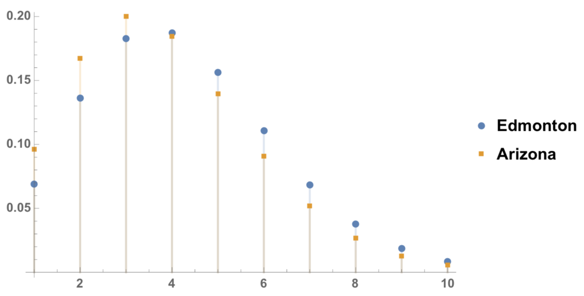
(b) We consider the posterior predictive densities using Equations (13) and (15) respectively. Therefore, we have

$$\begin{array}{c}\hfill X_{AB}\sim NB(51.5,0.924),X_{BA}\sim NB(34.5,0.90).\end{array}$$

(22)

In other words, making use of data from season $2017/18$ up to current date and specialists’ opinions, we are expecting Edmonton Oilers will score $3.25923$, while Arizona Coyotes scores $4.69523$.

Table 3. Winning probabilities of future upcoming match: Edmonton Oilers vs Arizona Coyotes based on specialists’ opinion and the dataset for season $2017/18$ and current season up to 29 January 2019.

${\pi }_w$	Probability that Edmonton Oilers wins the next match	$0.48$
${\pi }_l$	Probability that Arizona Coyotes wins the next match	$0.37$
${\pi }_d$	Probability that next match draws	$0.15$

and Figure 1 illustrate the result.

The most probable result is 4–3, in favor of Edmonton. Without using experts’ opinions, i.e., $d=0$, we have $X_{AB}\sim NB(34.5,0.96)$ and $X_{BA}\sim NB(23.5,0.9414)$, which corresponds to ${\pi }_w$ = 0.37, ${\pi }_l=0.35$ and ${\pi }_d=0.25$, respectively.

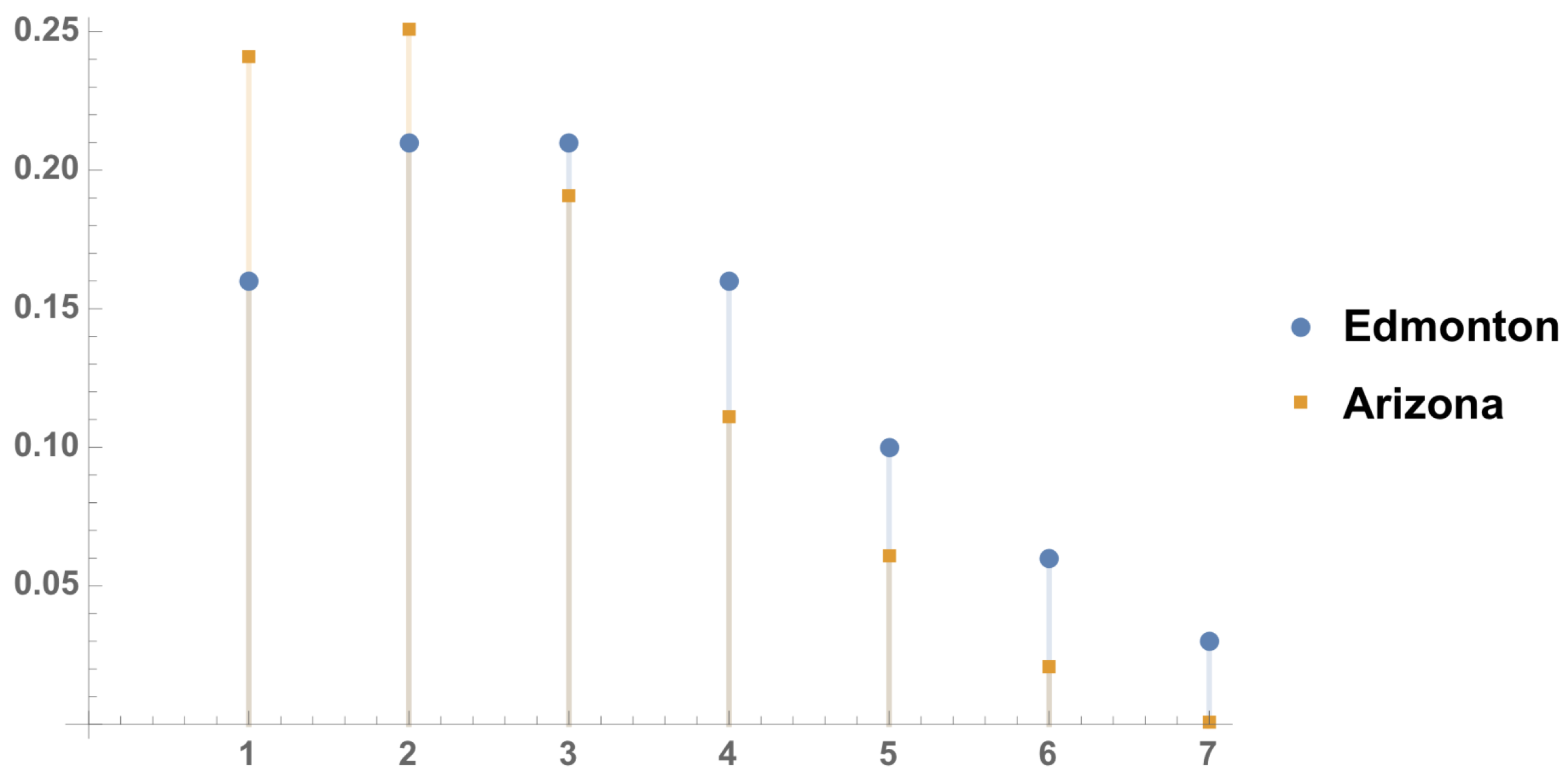
Assumption II:

Let us take $a=b=c=1$, $d=1$ and $r=0.9$. These choices result in having the expectation of $\lambda$ equals $3.88$ based on the prior distribution in (5). By applying (21), the posterior predictive densities of the number of the goals in the upcoming match Edmonton versus Arizona, along with corresponding plot, are given in

Table 4. Posterior predictive densities of number of goals scored by Edmonton versus Arizona.

x	0	1	2	3	4	5	6	7	8
$P(X_{AB}=x)$	0.06	0.16	0.21	0.21	0.16	0.1	0.06	0.03	0.01
$P(X_{BA}=x)$	0.13	0.24	0.25	0.19	0.11	0.06	0.02	0	0

and Figure 2.

Also from Table 4, we are expecting to see $1.96$ for Edmonton and $2.6$ goals for Arizona.

Table 5. Winning probabilities of future upcoming match: Edmonton Oilers vs Arizona Coyotes based on specialists’ opinion and dataset season 2017/18 and current season up to 29 January 2019.

${\pi }_w$	Probability that Edmonton Oilers wins the next match	$0.55$
${\pi }_l$	Probability that Arizona Coyotes wins the next match	$0.29$
${\pi }_d$	Probability that next match draws	$0.16$

shows the winning probabilities and one can predict that in the upcoming match, based on assumption II, Arizona will win the match in the Edmonton’s home, and most probable result is 3–2.

5.1. Prediction Errors

Prediction errors (pe’s) of our posterior predictive distributions in the two assumptions, when the specialists’ opinions matter, (namely ${\widehat{q}}_1\left(x_{AB}\right)$ and ${\widehat{q}}_2\left(x_{AB}\right)$ respectively) are evaluated by measuring the Kullback–Leibler distance as below.

$$\begin{array}{c}\hfill pe\left({\widehat{q}}_{i,AB}\right)={\mathbb{E}}^{X_{AB}}log\frac{q_{{\lambda }_{AB}}\left(x_{AB}\right)}{{\widehat{q}}_i\left(x_{AB}\right)},i=1,2,\end{array}$$

where $q_{{\lambda }_{AB}}\left(x_{AB}\right)$ is the Poisson distribution in (8) and ${\widehat{q}}_i\left(x_{AB}\right)$ for $i=1,2$ are given in (13) and (21), respectively. This can be repeated for ${\widehat{q}}_1\left(x_{BA}\right)$ and ${\widehat{q}}_2\left(x_{BA}\right)$ as well.

According to Table 1, one needs to calculate the distance between $Po\left(5\right)$ and $NB(51.5,0.924)$ regarding number of goals team A scores against team B and the distance between $Po\left(3\right)$ and $NB(34.5,0.90)$ regarding number of goals team B scores A in Assumption I. There we have $pe\left({\widehat{q}}_{1,AB}\right)=0.026$ and $pe\left({\widehat{q}}_{1,BA}\right)=0.033$. In contrast, if we follow Assumption II based on Table 4, the prediction errors become $pe\left({\widehat{q}}_{2,AB}\right)=0.18$ and $pe\left({\widehat{q}}_{2,BA}\right)=0.046$, respectively.

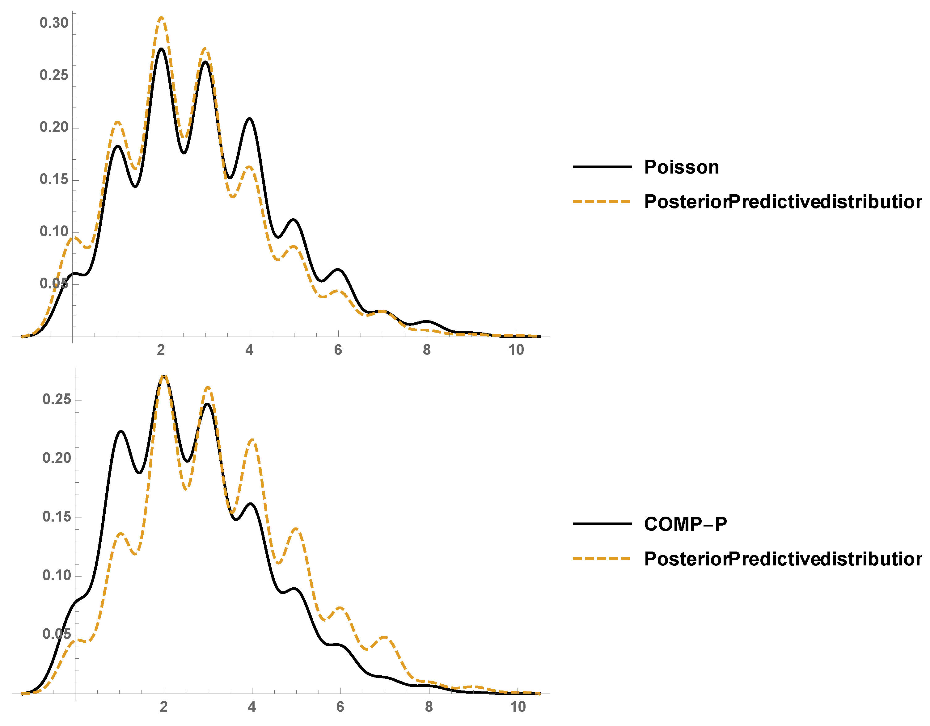
5.2. Simulation Study

We consider a small simulation study based on a sample of size of 1000, in order to investigate the proposed posterior density estimators regarding number of goals team B scores against team A in Section 5. Figure 3 depicts the assumed underlying model Po (Assumption I) and COM-P (Assumption II) along with their corresponding posterior predictive densities. It can be seen that model assumption I and its posterior predictive density estimator performs better for the number of goals.

6. Conclusions

In summation, we have proposed Bayesian predictive density estimators for the number of goals in a hockey match and consequently predicting the winner of the game. We considered two different assumptions and furthermore we considered points in previous games, away and home factors, and specialists’ opinions to improve our predictions. Assumption I, is based on that the underlying model, i.e., the number of goals in hockey, follows the Poisson distributions, and Assumption II considers the COM-P. However, based on prediction errors, it is easier to assume Assumption I. Eventually, the predictors based on either Assumption I or II, confirm that Edmonton (home team) will win game the next match versus Arizona (away team) by a difference of one goal with 48 and 55 percent, respectively.