Foreign Exchange Expectation Errors and Filtration Enlargements

Abstract

Extrapolations of future market forward rates are a better predictor of the 30-days ahead BRL-USD exchange rate than forecasts from the Central Bank Focus survey of Brazilian market participants. This is puzzling because market participants observe forward rates as they submit predictions, and thus these agents perform biased forecasts even though they have access to a set of unbiased forecasts, consistent with a martingale process for the exchange rate. We argue that this rational conundrum can be explained by a mechanism through which new information enlarges the information set (a filtration), changing the underlying measure and inducing a drift into the martingale process, turning the process into a strict local martingale and generating a forecast bias. Empirical results suggest that Focus survey forecasts indeed display characteristics of a strict local martingale, while spot exchange rates and forward rates are consistent with a martingale process.

1. Introduction

Imagine a rational agent that observes some information set (a filtration $\mathbb{F}={\left({\mathcal{F}}_t\right)}_{t\ge 0}$) and is interested in forecasting values of some random variable. As new information becomes available (in the form of a random variable L, such that we have a new, enlarged filtration $\mathbb{G}={\left({\mathcal{G}}_t\right)}_{t\ge 0}$ where ${\mathcal{G}}_t={\bigcup }_{ϵ>0}\left({\mathcal{F}}_{t+ϵ}\vee \sigma \left(L\right)\right)$, one would expect correction of systematic errors and/or some reduction of prediction variance. Through the information accumulation process useless information is discarded, and only information that yields true prediction gains is incorporated—one thus expects forecasts based on the enlarged information set $\mathbb{G}$ to be at least as good as forecasts based on the smaller information set $\mathbb{F}$. In this work we show an example where a larger set of information leads to a bias in the forecasting process, which seems in contradiction with the mechanism described above.

We compare survey-based forecasts from the Market Expectations System of the Central Bank of Brazil (henceforth Focus) with future markets (B3 futures exchange markets, former BMF and BOVESPA) 30-days forward rates; and find that future markets rates are unbiased predictor of future spot rates, but Focus survey forecasts are biased predictors through a substantial portion the observed sample. This is counter-intuitive because forward rates are obviously within the information set of keen market participants. No arbitrage theory asserts that exchange rates should be well characterized by a martingale process under the equivalent risk neutral measure P—i.e., the best possible predictor of future exchange rates is the present value of forward rates. Results in Section 3 suggest it is indeed the case in Brazilian markets; it is not possible to reject the martingale hypothesis for either the spot exchange rate, or future market forward rates. Yet Focus survey forecasts seem inconsistent with a martingale process. One could say that markets participants are employing a prediction scheme systematically incompatible with the observed stochastic process of interest. How to explain such phenomenon?

We argue this puzzling phenomenon can be interpreted through strict local martingale theory—specifically through the mechanism detailed by Dandapani and Protter [1]. Dandapani and Protter [1] explain how enlarging filtration F to G changes the underlying measure (say from P to Q), which can induce a stochastic drift in the volatility of S, turning S from an $\mathbb{F}$ martingale to a $\mathbb{G}$ strict local martingale.

The idea of smaller and larger information sets is natural to problems in finance. The filtration enlargements problem is studied in Jeulin and Yor [2], Jeulin [3] and Jeulin and Yor [4], and more recent developments in Aksamit and Jeanblanc [5]. As an example of application in finance Corcuera and Vadivia [6] show how filtration enlargements can be applied to model default risk and insider trading problems. Strict local martingales are at the core of a blooming real-time bubble detection literature. For example, Jarrow et al. [7] apply a nonparametric methodology (which we borrow in Section 4) to show that Linked-In stock exhibited price bubble behavior immediately after the firms IPO, and Chaim and Laurini [8] identify Bitcoin bubbles. Recent developments include, for example, Dandapani and Protter [9] who provide sufficient conditions for the multidimensional case, and Piiroinen et al. [10] who introduce a bubble detection indicator based on option prices.

Using two different identification techniques we explore the strict local martingale hypothesis. In Section 4 we employ a nonparametric kernel approach based on Jarrow et al. [11] to study how the volatility of our series of interest behave as price varies, and access the convergence of condition (3). We then turn to an alternative, parametric strict local martingale test in Section 5.

To our knowledge this is the first work to relate systematic prediction errors and the filtration enlargement mechanism. While the nonparametric identification procedure in Section 4 draws heavily from Jarrow et al. [11], formal univariate estimation of the stochastic volatility model in Section 5 is itself novel. Standard practice in financial industry is to calibrate parameter values from option price information (see for example Mikhailov and Nögel [12]), and classical estimates (like by Ait-Sahalia and Kimmel [13]) employ volatility proxies to circumvent the latent variable problem—we tackle the latent variable issue by employing Bayesian simulation techniques to estimate model 13, so that it is possible to make inference regarding model parameters from a single time series.

The remainder of this paper is structured as follows. Section 2 presents some key definitions and a discussion about the filtration enlargement mechanism. Empirical evidence of our main points are found in Section 3. Nonparametric strict local martingale identification is presented in Section 4. Section 5 details our parametric estimation. We discuss results in Section 6, and Section 7 concludes.

2. Filtration Enlargement and Strict Local Martingales

2.1. Strict Local Martingales

A local martingale is a stochastic process, $M={\left(M_t\right)}_{t\ge 0}$, for which there exists an increasing sequence of stopping times ${\tau }_n\to \infty$ such that the stopped process $M_{min}\{\tau ,{\tau }_n\}$ is a martingale with probability one. The key insight is that if M is a local martingale, then it is either a true martingale or a strict local martingale (SLM).

The risky asset price, $S={\left(S_t\right)}_{t\ge 0}$, is assumed non-negative and driven by a standard stochastic differential equation

$$d{S}_t=\sigma \left(S_t\right)d{W}_t+\mu \left(S_t\right)dt.$$

(1)

No arbitrage in the sense of “no free lunch with vanishing risk” (Delbaen and Schachermayer [14]) implies that there exists a risk neutral measure under which the SDE in (1) simplifies to

$$S_t=S_0+{\int }_0^t\sigma \left(S_s\right)dWs.$$

(2)

A very important property (to be further exploited) is that S is a strict local martingale if and only if

$${\int }_{\alpha }^{\infty }\frac{x}{\sigma {\left(x\right)}^2}dx<\infty$$

(3)

for all $\alpha >0$. Jarrow [15] notes that condition in Equation (3) states that an asset is a strict local if and only if its volatility, as function of its price, increases faster than linearly.

Jarrow et al. [11] discuss the intuition behind the distinction between a non-negative martingale and a strict local martingale, $S\ge 0$, follows from the fact that S is always a supermartingale and is a true martingale if and only if it has constant expectation. Then if S is a strict local martingale its expectation decreases over time. The typical behavior of a SLM process is to shoot up to high values, to then drop down and stay low.

2.2. Filtration Enlargement

Dandapani and Protter [1] detail a mechanism through which new information introduced into the observed information set (the initial filtration $\mathbb{F}$) induce a change in the measure, from P under $\mathbb{F}$ to Q under the enlarged filtration $\mathbb{G}$, such that a $\mathbb{F}$ martingale process S can become a $\mathbb{G}$ strict local martingale for a random time interval.

To understand how the filtration enlargement mechanism connects strict local martingale bubbles and systematic foreign exchange forecast errors, imagine some agent one wants to predict future values of a risky asset $S={\left(S_t\right)}_{t\ge 0}$ (for example the 30-days spot BRL-USD exchange rate). Agent one observes an information set (a filtration) $\mathbb{F}={\left({\mathcal{F}}_t\right)}_{t\ge 0}$, such that we have a complete filtered probability space $(\mathsf{\Omega },\mathcal{F},\mathbb{F},P)$. Suppose S is a $\mathbb{F}$ true martingale under measure P.

Now consider some other agent two that also aims to forecast S. At time $t=0$ only agent Two observes a random variable L, that enlarges her information set, from $\mathbb{F}$ to $\mathbb{G}={\left({\mathcal{G}}_t\right)}_{t\ge 0}$—i.e., $L\in \mathbb{G}$ but $L\notin \mathbb{F}$. Dandapani and Protter [1] show that it is possible for, due to such change, process S to be a $\mathbb{G}$ strict local martingale. The mechanism that allows the construction of a strict local martingale is a class of stochastic volatility model, detailed below.

Consider the Heston type model studied by Lions and Musiela [16]

$$\begin{array}{cc}\hfill d{S}_t\hfill & \hfill =S_t{v}_{t}d{B}_t\hfill \end{array}$$

(4)

$$\begin{array}{cc}\hfill d{v}_t\hfill & \hfill =\sigma \left(v_t\right)d{W}_t+b\left(v_t\right)dt,\hfill \end{array}$$

(5)

where $d{B}_t$ and $d{W}_t$ are two correlated Brownian motions with correlation parameter $\rho$. Denote the new, enlarged filtration $\mathbb{G}$ as

$${\mathcal{G}}_t=\bigcap _{ϵ>0}\left({\mathcal{F}}_{t+ϵ}\vee \sigma \left(L\right)\right).$$

Let $\eta$ be the distribution of L, and $Q_t(w,dw)$ be the regular conditional distribution of L given ${\mathcal{F}}_t$. There exists an $\mathbb{F}$ martingale $q^x(t,w)\eta \left(d_x\right)$ which is a version of $Q_t(w,dx)$. If S is an $\mathbb{F}$ martingale, then there exists an F predictable process $k^x(t,2)$, such that

$$[q^x,S]=\left(k^x{q}_{\_}^x\right)·[S,S].$$

(6)

Jacod [17] shows that the following process ${\widehat{S}}_t$ is a $\mathbb{G}$ local martingale

$${\widehat{S}}_t=S_t-{\int }_0^t{k}_d^{L}d{[S,S]}_s.$$

(7)

Enlarging filtration $\mathbb{F}$ to $\mathbb{G}$ changes the semimartingale decomposition of both S and v. Girsanov’s theorem allows us to restore the local martingale properties of S by changing the equivalent probability measure to Q.

Under $(Q,\mathcal{G})$, S can be written as

$$\begin{array}{c}{S}_t={\int }_0^t\left(S_s{v}_s\right)d{B}_s-{\int }_0^t{k}_s^L{\left(S_s{v}_s\right)}^2{d}_s\hfill \\ -{\int }_0^t(\left(S_s{v}_s\right)H_s+\rho J_s)d_s+{\int }_0^t{k}_s^L{\left(S_s{v}_s\right)}^2{d}_s+{\int }_0^t(\left(S_s{v}_s\right)H_s+\rho J_s)ds,\hfill \end{array}$$

(8)

to ensure that S is a Q local martingale we choose

$$k_t^L{\left(S_t{v}_t\right)}^2=-\left(S_t{v}_t\right)H_t-\rho J_t.$$

(9)

The drift component $b\left(v_t\right)$ in volatility Equation (5) also changes

$$\widehat{b}\left(v_t\right)=b\left(v_t\right)+k_t^L{\sigma }^2\left(v_t\right)+(\rho H_t+J_t)\sigma \left(v_t\right).$$

(10)

This is the change in the drift of the volatility equation that enables the change from a martingale to a strict local martingale.

We can now state Theorem 3 of Dandapani and Protter [1] (p.p. 10), which relates S local martingale under $(\mathbb{F},P)$ to S strict local martingale under $(\mathbb{G},Q)$.

Theorem 1.

Dandapani and Protter [1]. Assume that $k,H$ and J have right continuous paths almost surely, and $Q(w:k_0^L>0)>0$. Suppose functions $\sigma (·)$ and $b(·)$ are ${\mathcal{C}}^1$, and the following two conditions hold:

$$\begin{array}{cc}\hfill \hfill & \hfill \underset{x\to +\infty }{lim\; sup}\frac{\rho x\sigma \left(x\right)+b\left(x\right)}{x}<\infty \hfill \end{array}$$

(i)

$$\begin{array}{cc}\hfill \hfill & \hfill \underset{x\to +\infty }{lim\; inf}\left(\rho x\sigma \left(x\right)+b\left(x\right))+min({\epsilon }^{\left(1\right)},{\epsilon }^{\left(2\right)}){\sigma }^2\left(x\right)-max({\epsilon }^{\left(1\right)},{\epsilon }^{\left(2\right)})\sigma \left(x\right)\right){\varphi }^{-1}\left(x\right)\ge 0,\hfill \end{array}$$

(ii)

where $\varphi \left(x\right)$ is an increasing, positive, smooth function satisfying

$${\int }_{\alpha }^{\infty }\frac{1}{\varphi \left(x\right)}dx<\infty .$$

Let S be the unique strong solution of the SDE

$$\begin{array}{c}d{S}_t=S_t{v}_{t}d{B}_t\hfill \\ d{v}_t=\sigma \left(v_t\right)d{W}_t+b\left(v_t\right)d_t,\hfill \end{array}$$

on (P,$\mathbb{F}$), where $B_t$ and $W_t$ are Brownian motions with correlation $\rho >0$. Then process S is also the solution of

$$\begin{array}{c}d{S}_t=S_t{v}_{t}d{B}_t\hfill \\ d{v}_t=\sigma \left(v_t\right)d{W}_t+b\left(v_t\right)d_t+k_t^L{\sigma }^2\left(v_t\right)d_t+(\rho H_t+J_t)\sigma \left(v_t\right)d_t.\hfill \end{array}$$

Proof. 

See Dandapani and Protter [1]. □

Therefore if functions $\sigma (·)$ and $b(·)$ respect conditions (i) and (ii), then under the enlarged filtration $\mathbb{G}$ the drift component $b(·)$ changes to $\widehat{b}(·)$ (as in Equation (10)), which turs S from an $\mathbb{F}$ (true) martingale into a $\mathbb{G}$ strict local martingale.

The presence of stochastic volatility in financial series is an important stylized fact in the field of finance. In the following sections we show that the characterization of a strict local martingale through a stochastic volatility model is consistent with the behavior observed in the forecasts for the foreign exchange market studied in this article, and thus can be a valid explanation for the observed forecast bias.

3. Empirical Evidence

Our sample consists of (30-days ahead) exchange rate predictions of Brazilian market participants (the Focus survey); future markets closing forward rates traded at B3 (former Bovespa BMF); and the official Brazilian exchange rate (PTAX). Sample range and frequency are limited by Focus data such that 179 monthly observations, from November 2001 to September 2016, are available. The data used in this work are available on the websites of the Central Bank do Brazil and B3.

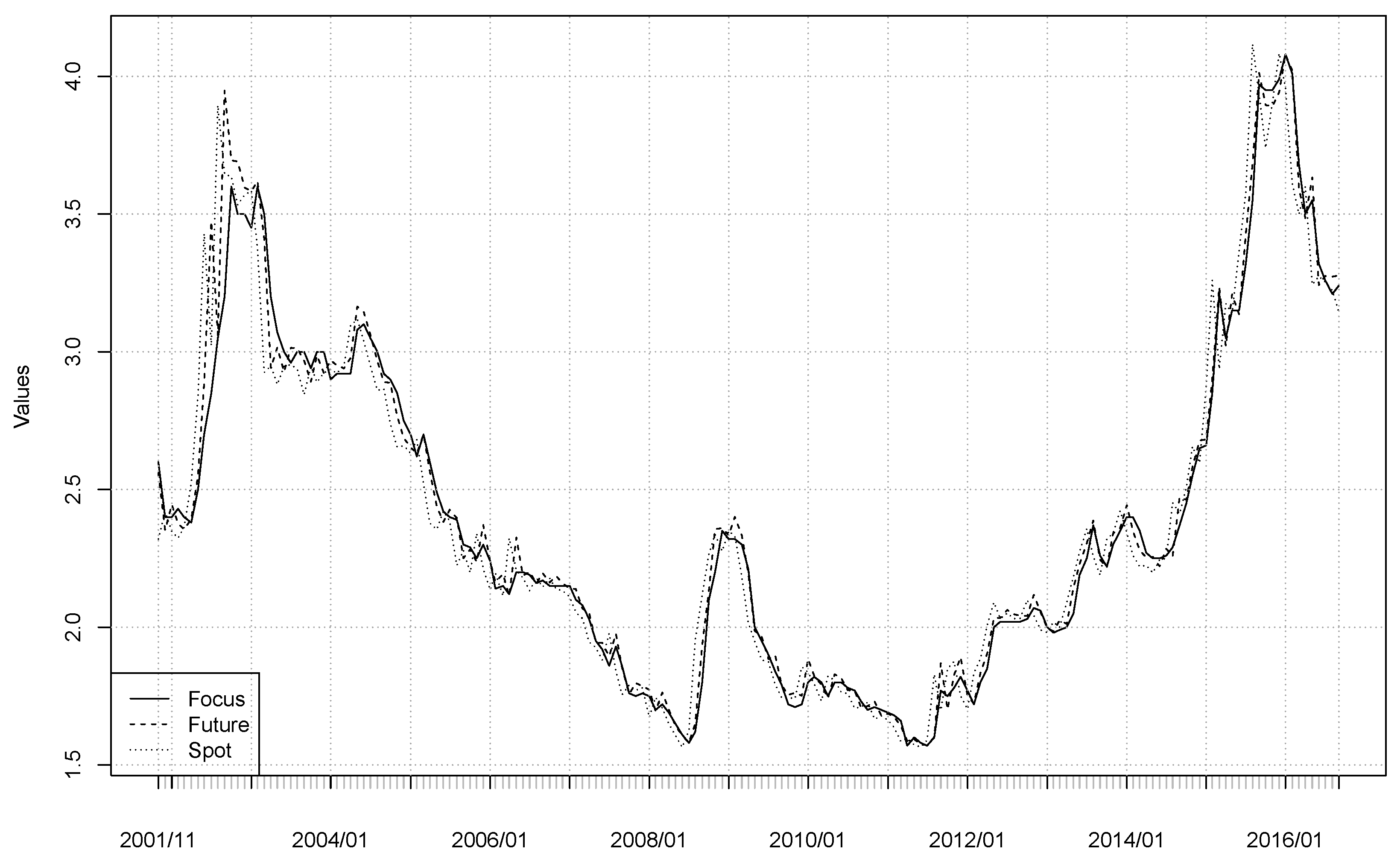
Focus forecasts regard the last week day of the corresponding month, while future markets forward rates are for the first week day of the same month. We thus obtained the “predicted forward rate at the last day of the month” by using the Brazilian interbank deposit certificate (CDI) rate. We also considered two alternative formulations—first using the forward rate the day before Focus release, and then using the forward two months maturity. Results were similar to the baseline formulation and therefore not reported. Trajectories are plotted in Figure 1, and descriptive statistics are displayed in

Table 1. Descriptive statistics.

	Mean	SD	Max	Min	MFE
Spot	2.397	0.630	4.117	1.564	0.000
Focus	2.393	0.625	4.080	1.570	−0.004
Future	2.414	0.636	4.079	1.572	0.017

Note: This table reports descriptive statistics for BRL-USD (PTAX) spot exchange rates, BMF and BOVESPA CDI-discounted forward rates, and Focus forecasts. Mean forecast error (MFE) is with respect to spot exchange rates.

.

The Focus Bulletin is a survey released every Monday by the Central Bank of Brazil. The report, a daily survey of forecasts of about 120 banks, funds and other institutions summarizes the market expectations for the Brazilian economy. The market expectations system, which collects information reported in the Focus Bulletin, consists of a web interface where agents report their expectations for the macroeconomic variables of interest. The system considers the last information reported in the past 30 days by market participants. If an agent does not revise his or her expectations in the last thirty days, this information is not considered in statistic calculations. An important incentive of this system is the monthly release of best performing institutions, indicated in the top five predictors for each macroeconomic variable monitored in the system (see Mariani and Laurini [18] for a thorough description of the Focus survey).

We now verify whether processes describing forward rates, Focus forecasts, and the spot exchange rate are consistent with a martingale process—as expected by the first theorem of asset pricing. For this we employed test-based on Cramer–von Mises (CvM) and Kolmogorov–Smirnov (KS) statistics proposed by Domínguez and Lobato [19], augmented with bootstrap finite sample correction of Charles et al. [20]. Test statistics and equivalent p-values are reported in

Table 2. Martingale tests.

	CvM	CvM p-val	KS	KS p-val
Focus	2.569	0.000	2.282	0.000
Future	0.042	0.948	0.553	0.897
Spot	0.070	0.810	0.731	0.616
$\Delta$ Focus	2.730	0.000	2.150	0.000
$\Delta$ Future	0.026	0.990	0.549	0.910

Note: This table reports martingale tests of BRL-USD (PTAX) spot exchange rates, B3 (BMF and BOVESPA) CDI-discounted forward rates, and Focus survey forecasts. Cramer–von Mises (CvM) and Kolmogorov–Smirnov statistics calculation were based in 2000 bootstrap replications.

. Both tests failed to reject the martingale null hypothesis for the spot exchange rate and future markets forward rates, but rejected it when considering Focus forecasts. The same tests were applied to prediction errors (future-spot and Focus-spot). We find that the difference martingale hypothesis was rejected for Focus prediction errors, and not rejected for future market prediction errors. This result indicated that there was a systematic bias component in the forecasts reported in the Focus system, which was inconsistent with the behavior of spot and future exchange rates, and indicated that Focus forecasts were sub-optimal.

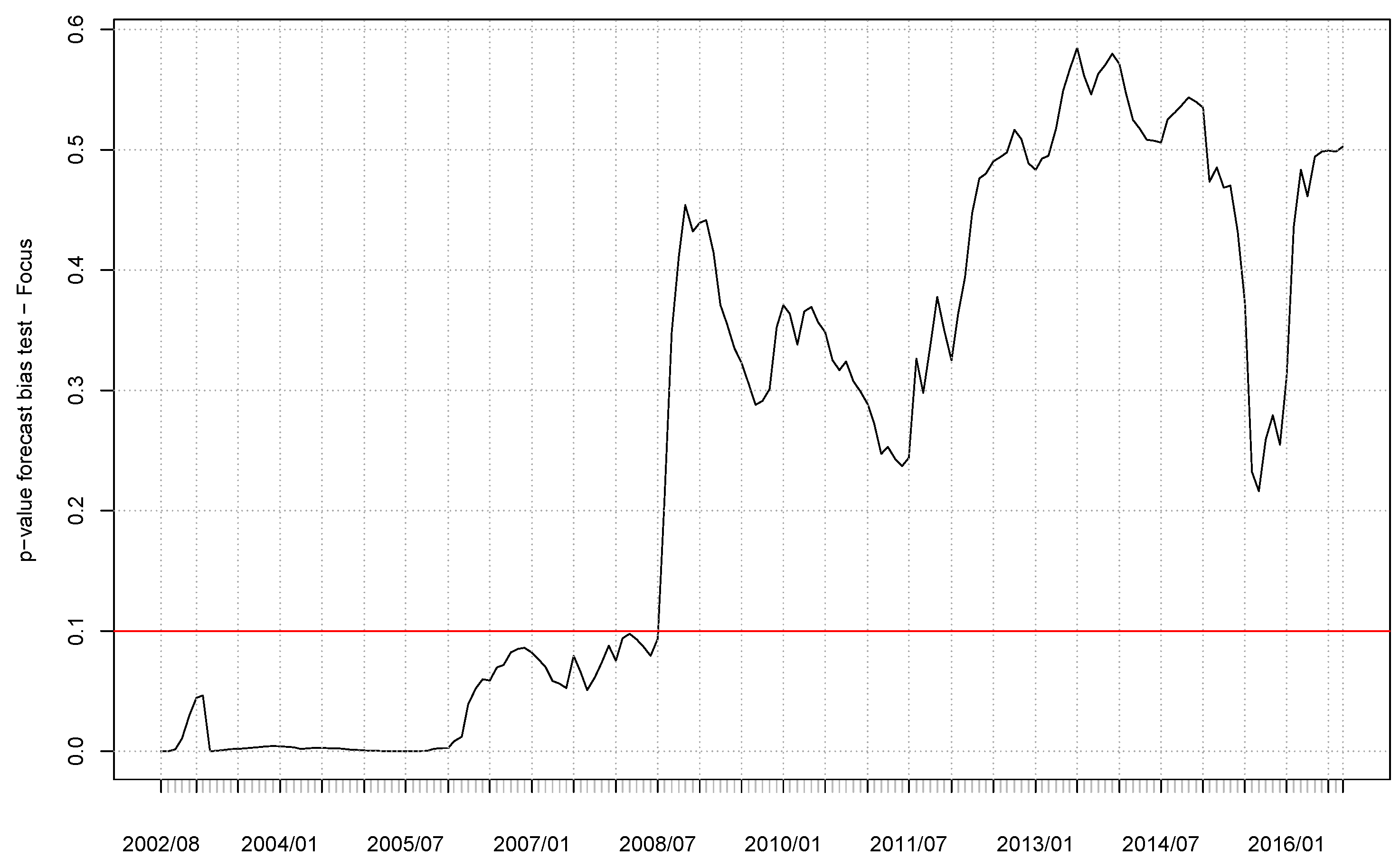
Figure 2 plots p-values for a rolling-sample forecast bias test. We regress 30-days ahead exchange rates against Focus forecasts and a constant, i.e., $y_t=\alpha +\beta x_t+{\epsilon }_t$, and jointly test if $\alpha =0$ and $\beta =1$. From November 2001 to July 2008 it was possible to reject the null $\alpha =0$ and $\beta =1$ hypothesis at a $10\%$ significance level, again supporting the existence of a relevant bias in the forecasts of market analysts reported in the Focus system.

Table 3. Forecast comparison.

	ME	RMSE	MAE
Focus	−0.004	0.159	0.102
Future	0.017	0.146	0.096
Focus first subsample	0.011	0.182	0.110
Future first subsample	0.035	0.167	0.105
Focus second subsample	−0.016	0.136	0.095
Future second subsample	0.002	0.126	0.088

Note: This table reports BRL-USD (PTAX) spot exchange rates prediction performance comparison statistics of BMF and BOVESPA CDI-discounted forward rates, and Focus forecasts. We split the observed sample in two sub-samples, 2001/08 to 2008/07, and from 2008/08 forwards. Column one displays mean error, second column root mean squared error, third column mean absolute error.

displays an illustrative prediction performance comparison between Focus survey forecasts and future market rates. We repeat the procedure for the “biased” and “unbiased” Focus subsamples (30 November 2001–31 July 2008 and 29 September 2008–30 September 2016). Forward rates were generally a better predictor the 30-days ahead spot interest rate. When considering the whole sample or any subsample forward rates fared better when considering RMSE or MAE, while Focus mean prediction errors were smaller in absolute terms.

For each subsample we tested the null hypothesis of no difference in forecast accuracy by using the Diebold and Mariano [21] and Clark and West [22] tests. From p-values in

Table 4. Forecast tests.

	DM	CW
Full Sample	0.0154	<1 ×${10}^{-3}$
First Subsample	0.0294	<1 ×${10}^{-3}$
Second Subsample	<1 × 10−3	<1 ×${10}^{-3}$

Note: This table displays p-values of Diebold and Mariano [21] (DM) and Clark and West [22] (CW) tests. The DM test has the null hypothesis of equality of predictive performance, against the alternative of better predictive performance for the first model (Future market forecasts). Tests employ quadratic loss function.

we can see the null of equal forecast performance was rejected at 5% by both tests for all subsamples. Indeed, Clark and West [22] tests rejected the null at the 1% level for all subsamples; and p-values of Diebold and Mariano [21] were always smaller than 0.03. These results reinforced that forward rates were indeed better predictors of 30-days ahead spot rates than Focus survey forecasts.

In the following sections we show that this bias component can be explained by the presence of a strict local martingale, using the framework proposed in Dandapani and Protter [1]. For this we used non-parametric and parametric tests for the presence of an SLM, verifying the existence conditions in the volatility structure of the price process.

4. Nonparametric Estimation

Recall from our discussion in Section 2 that a stochastic process is a strict local martingale if its volatility increases fast enough with higher level, such that

$${\int }_{\alpha }^{\infty }\frac{x}{{\sigma }^2\left(x\right)}dx<\infty ,$$

(11)

for all $\alpha >0$. We tried to empirically characterize the volatility term $\sigma {\left(x\right)}^2$ in order to study the convergence properties of the integral above. In order to estimate ${\sigma }^2\left(S_t\right)$ and relation (3), we employed the kernel-based estimator of Florens-Zmirou [23] and Jiang and Knight [24] for the diffusion component:

$${\widehat{\sigma }}^2\left(x\right)=\frac{{\sum }_{i=0}^{n-1}K\left(\frac{x-X_i}{h_n}\right){\left(X_{i+1}-x\right)}^2}{{\Delta }_n{\sum }_{i=0}^{n-1}K\left(\frac{x-X_i}{h_n}\right)},$$

(12)

where $K(·)$ is a kernel function with bandwidth $h_n$. Is this work we used a Gaussian kernel and generalized cross-validation to estimate the optimal bandwidth parameter.

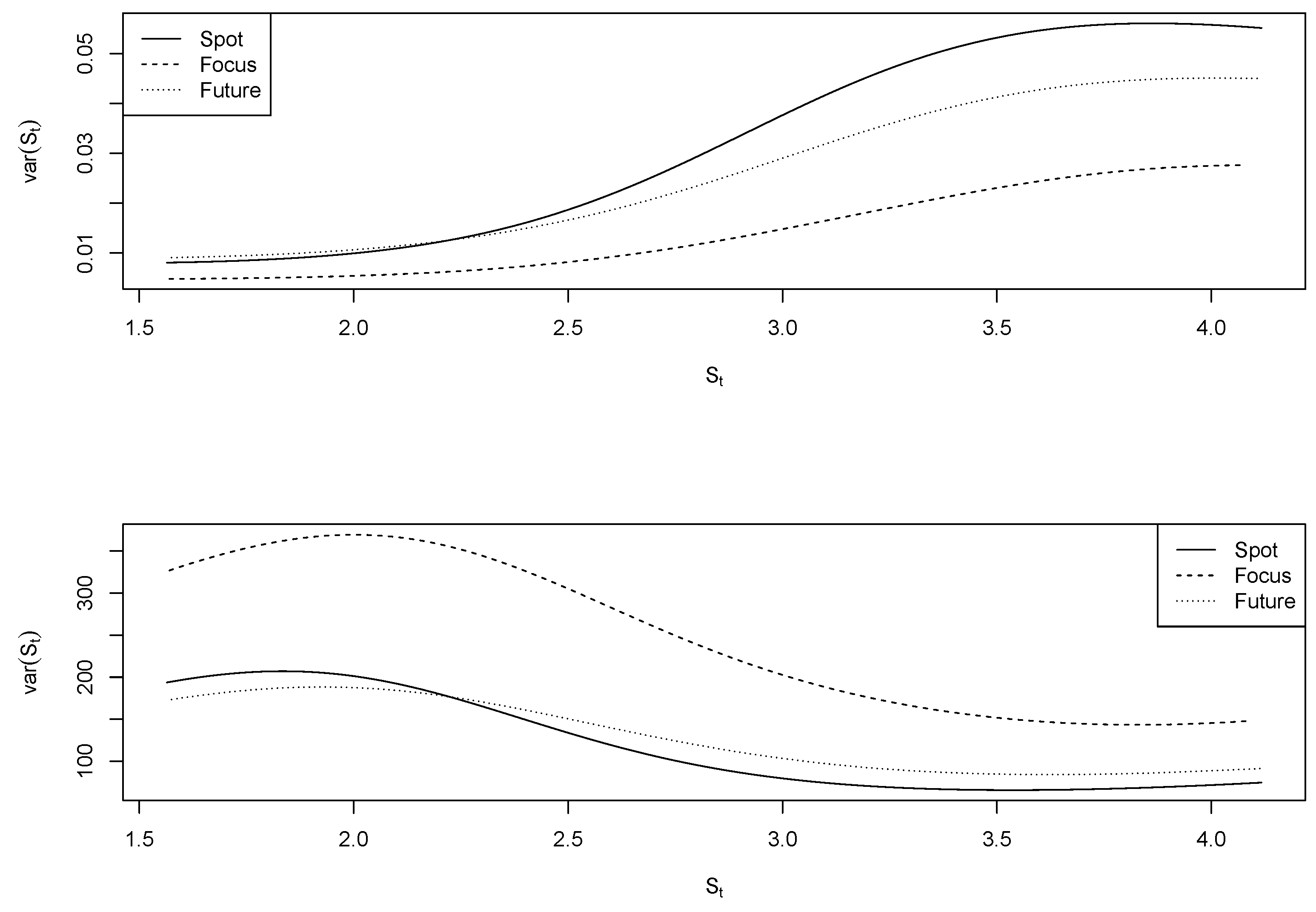
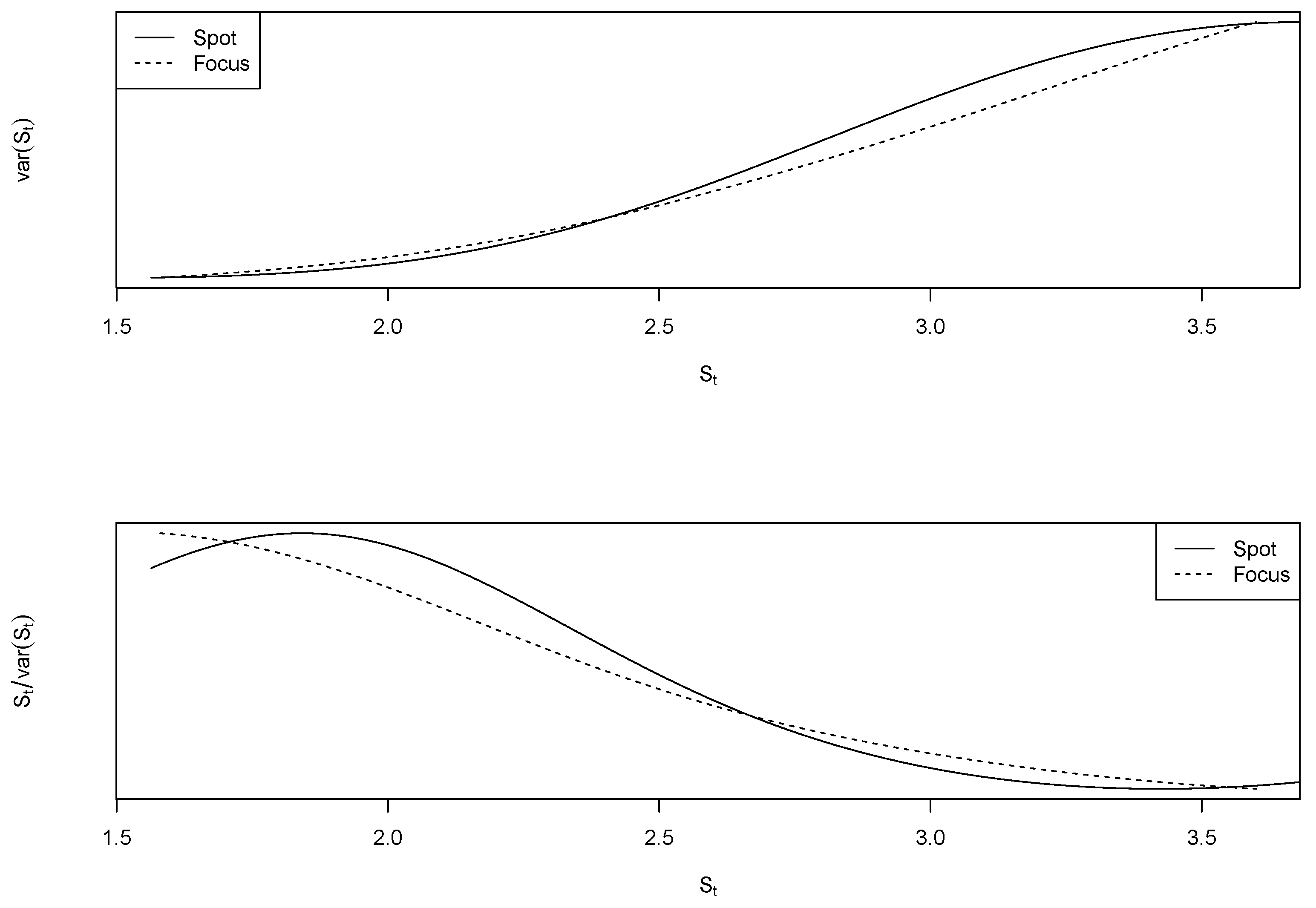
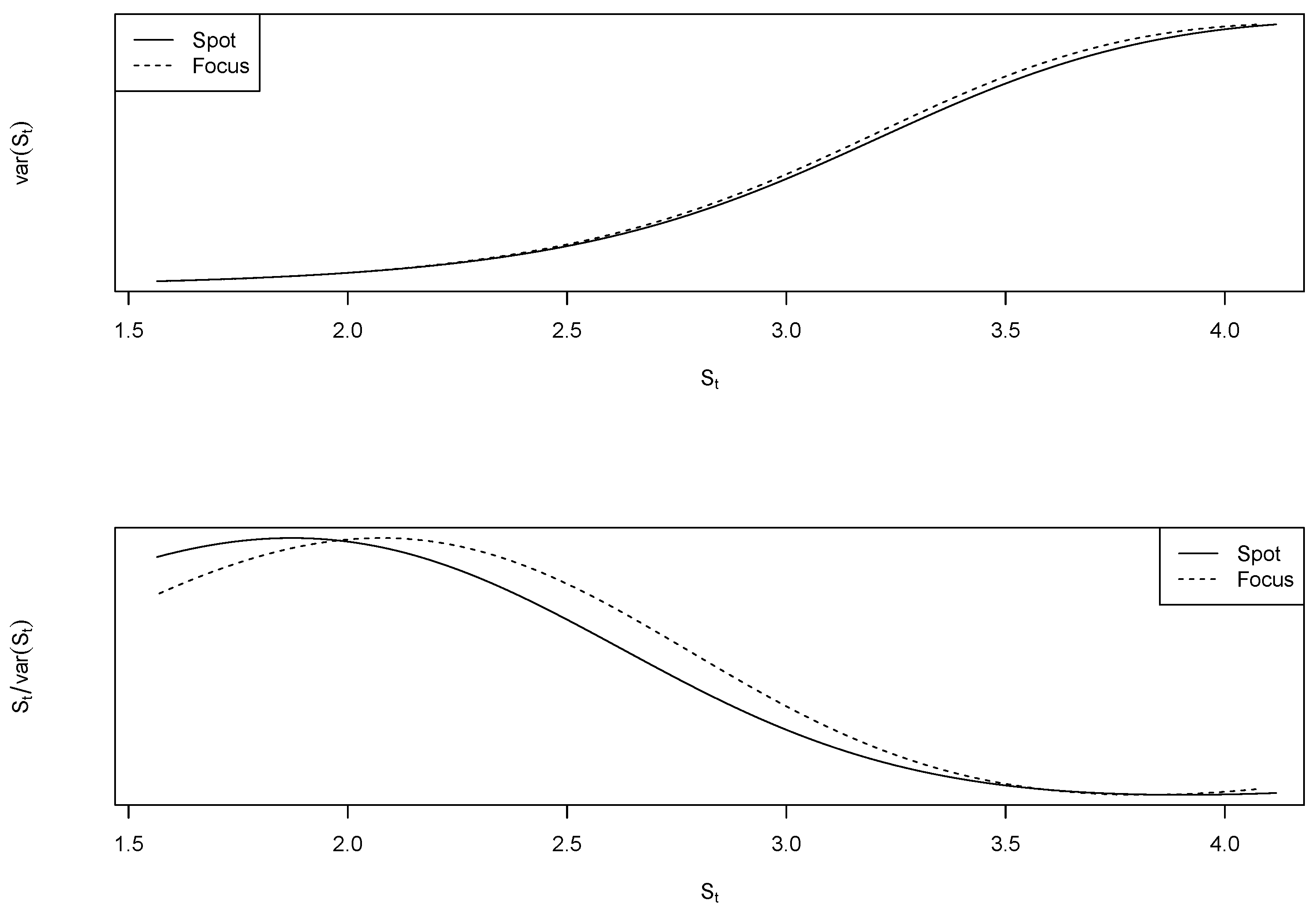
Figure 3 and Figure 4 plots estimated volatility functions (top panel) and relation $x/{\sigma }^2\left(x\right)$ (bottom panel), for our three processes of interest. One readily notices that Focus forecasts were less volatile than spot exchange rates or future market predictions for every observed price realization, and that volatility functions of both spot rates and future markets stopped increasing somewhere past the $x=3.75$ mark. The relation $x/{\sigma }^2\left(x\right)$ was stable (one might even say increasing) at higher price ranges for spot and future processes, which alludes to a violation of the condition in Equation (3) (i.e., the integral is infinite)—indicating that spot rates and future market predictions are true martingales.

The curvature of the volatility function of Focus forecasts decreased slower, such that the function was always increasing for observed prices. This reduces the term $x/{\sigma }^2\left(x\right)$ and indicates convergence of the integral in Equation (3).

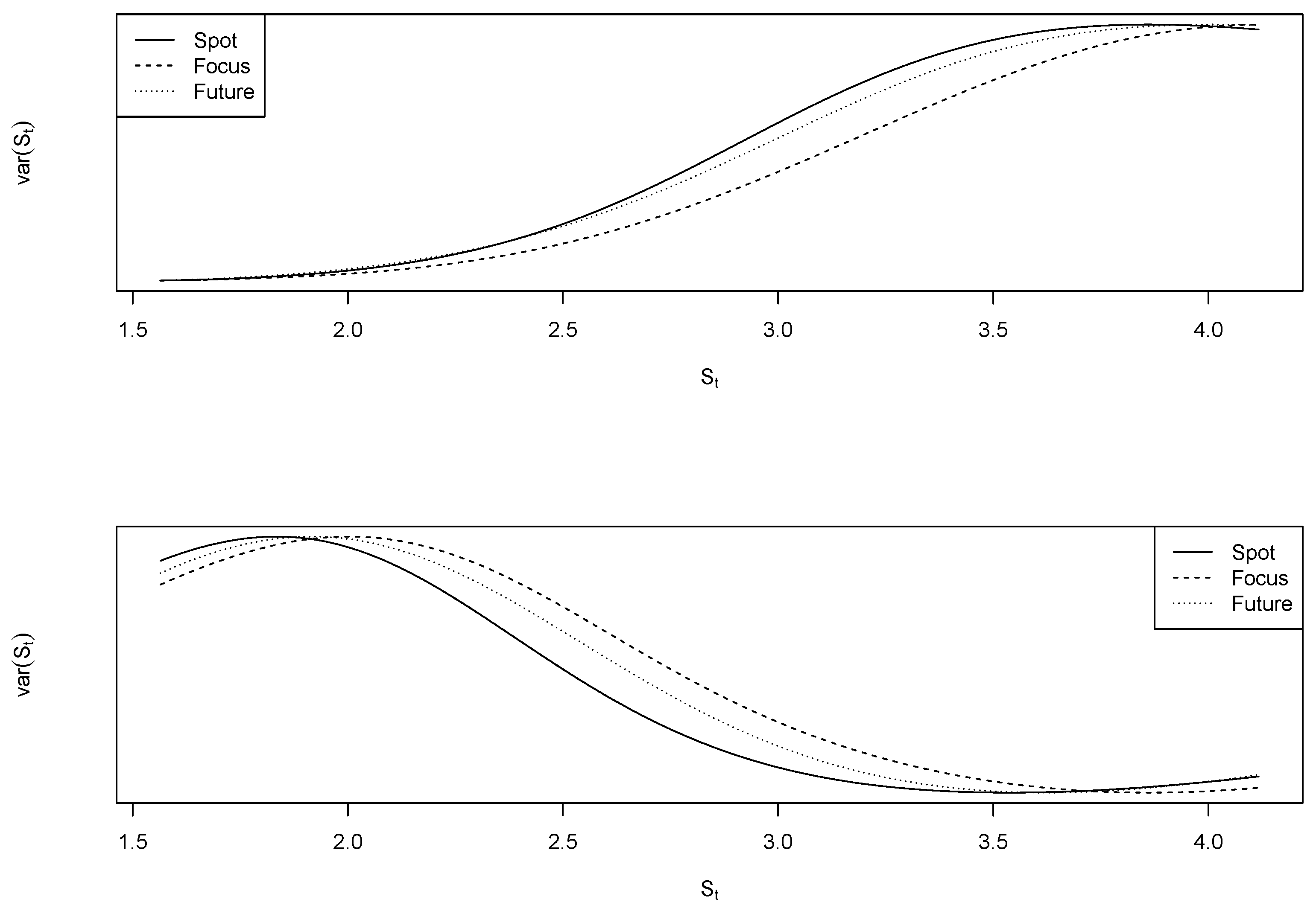
We argue systematic Focus prediction errors are associated with incompatibility between the stochastic process that drives forecasts and exchange rates. Figure 5 plots ${\sigma }^2\left(x\right)$ and $x/{\sigma }^2\left(x\right)$ for the first subsample period. Note the absence of inflection at the end of Focus’ variance function, and how sharply $x/{\sigma }^2\left(x\right)$ decreases. This can be taken as evidence that Focus forecasts behaved like strict local martingales from November 2001 to August 2008. Conversely, when considered the second subsample, as in Figure 6, it becomes hard to distinguish between Focus and spot processes—both are consistent with what is to expect from true martingales.

This nonparametric analysis has some important limitations. First, the analysis is visual and presents no formal test for the SLM hypothesis. The second point is that the SLM behavior refers to extrapolation for the whole set of unobserved prices, whereas we only analyzed the variance function for observed sample values. To circumvent this limitation, we present a formal parametric test, detailed in the next section.

5. Parametric Estimation

Consider the stochastic volatility model studied by Andersen and Piterbarg [25]

$$\begin{array}{c}d{S}_t=\lambda S_t\sqrt{V_t}d{W}_t^1\hfill \\ d{V}_t=\kappa (\theta -V_t)dt+ϵV_t^{p}d{W}_t^2,\hfill \end{array}$$

(13)

where $\lambda ,\kappa ,\theta >0$ and $(W_t^1,W_t^2)$ is a standard two dimensional Brownian motion with correlation coefficient $\rho$. Note that if $p=1/2$ the model in Equation (13) reduces to the well-known Heston [26] model. This model is equivalent to the one discussed in Section 2, but also allows for testable implication of the Martingale hypothesis. Results of Andersen and Piterbarg [25] and Protter [27] describe how the parameter space of model (13) can be divided in two disjoint sets, such that a specific parameter range characterizes stochastic process S as a strict local martingale.

Theorem 2.

Andersen and Piterbarg [25]. For the model (13): if $\rho \le 0$, S is a true martingale; if $\rho >0$ and $p\le 1/2$ or $p>3/2$, S is a true martingale; if $\rho >0$ and $1/2<p<3/2$, then S is a strict local martingale. For the case $p=3/2$S is a true martingale if $\rho \le 1/2ϵ{\lambda }^{-1}$, and S is a strict local martingale if $\rho >1/2ϵ{\lambda }^{-1}$. Proof: see Protter [27].

Equipped with this theorem we employed Bayesian techniques to estimate the stochastic volatility model of Andersen and Piterbarg [25] to investigate whether Focus forecasts are compatible with a true martingale or a strict local martingale process.

Estimation was carried out in the Stan software (with help of the R-package “rstan"). Stan employs a Hamiltonian Monte Carlo (HMC) algorithm rather than the traditional Metropolis Hastings (MH). HMC augments the usual random walk posterior sampling scheme with Hamiltonian dynamics, such that new proposed values can be further apart than they would be under a random walk exploration scheme, but have a high acceptance probability nevertheless. HMC is then more efficient than MH in the sense that it takes fewer algorithm iterations in order to achieve chain convergence. This is especially relevant in our stochastic volatility context because Bayesian statistics treats latent variables as it treats unknown parameters, what can be computationally expensive.

We elected prior distributions given restrictions on parameter values in model (13). A Uniform distribution between 0 and $1.5$ was specified for $\lambda$ and $ϵ$; $\kappa$ was assumed Normal, with mean $0.9$ and standard deviation $0.5$; $\theta$ was assumed Normal, with mean $0.01$ and standard deviation $0.05$; p was also assumed Normal, with mean $0.5$ and standard deviation $0.05$; correlation $\rho$ was specified as $2{\rho }^{\ast }-1$, ${\rho }^{\ast }\sim Beta(5,2.5)$.

Table 5. Estimation results, unrestricted model.

	Mean	Std	0.025q	0.5q	0.975q
$\lambda$	0.630	0.378	0.137	0.552	1.416
$\kappa$	0.748	0.194	0.280	0.792	0.990
$\theta$	0.168	0.119	0.048	0.123	0.468
$ϵ$	0.826	0.348	0.273	0.799	1.452
$\rho$	0.226	0.180	0.026	0.174	0.667
p	0.365	0.204	0.028	0.364	0.743

Note: This table report results for the unrestricted estimation of model (13). First column displays posterior means, second column standard errors, and columns three through five display selected quantiles. Estimation was carried out by Hamiltonian Monte Carlo with 100,000 replications.

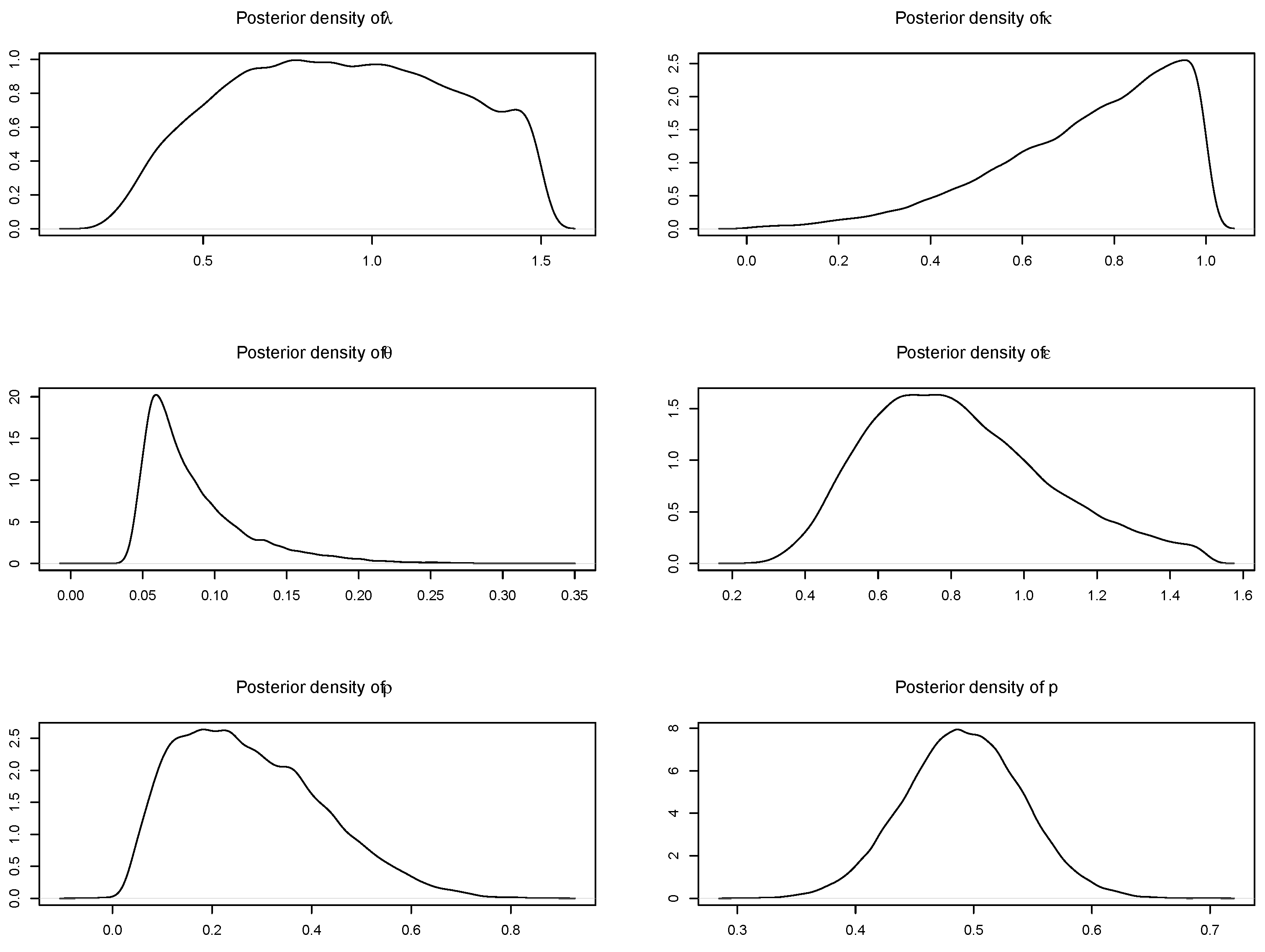
reports estimation results, posterior densities are displayed in Figure 7. Notice correlation coefficient $\rho$ was estimated positive inside the $95\%$ credible interval—this is desirable since if $\rho \le 0$, $S_t$ is a true martingale for all values of p, and further analysis would be unnecessary.

The posterior mean of parameter p is estimated around $0.365$, which according to Theorem 2 characterizes Focus forecasts as a true martingale process. However, the posterior distribution of p is quite disperse and imply substantial uncertainty regarding parameter value. Also, prior and posterior distributions of parameters $\lambda$ and $ϵ$ are very similar, thus it is questionable whether those parameters are identifiable from data.

We recognize that available Focus data is of monthly frequency and sample size is limited, which makes estimating model (13) an ambitious enterprise. In face of this identification difficulty we decided to fix $\lambda =1$ and focus attention on estimates of p and $\rho$, which were at the core of our parametric approach. This restriction was also used in Baldeaux et al. [28] and Chaim and Laurini [8], which also attempted to verify the presence of strict local martingales.

One can see from

Table 6. Estimation results, restricted model.

	Mean	Std	0.025q	0.5q	0.975q
$\kappa$	0.743	0.199	0.262	0.788	0.991
$\theta$	0.095	0.037	0.048	0.088	0.186
$ϵ$	0.789	0.291	0.340	0.747	1.408
$\rho$	0.194	0.093	0.062	0.178	0.415
p	0.507	0.046	0.413	0.507	0.597

Note: this table report results for the restricted ($\lambda =1$) estimation of model (13). First column displays posterior means, second column standard errors, and columns three through five display selected quantiles. Estimation was carried out by Hamiltonian Monte Carlo with 100,000 replications.

that the restricted model indeed yields more precise estimates. Comparing the second column of Table 5 and Table 6 one can see that posterior standard errors of $\theta$, $\rho$, and p were substantially smaller; while $\kappa$ estimates were essentially unchanged. Figure 8 displays bell-shaped, less disperse, posterior distributions of $\kappa$, $\rho$, and p.

Parameter p is now estimated between $0.4$ and $0.6$ with $95\%$ probability, a much narrower credibility interval. Still, because substantial probability was attributed to the $p\le 0.5$ range, it is not possible to convincingly assert that $S_t$ is a strict local martingale process from Table 6 alone. A more formal test is appropriate. We ask: does imposing that $S_t$ is a strict local martingale worsen fit performance? for such we further restrict model (13) such that $p\in \left[0.5,1.5\right]$. Then compare this formulation to the one in Table 6 and Figure 8, for which $p\in [0.5,\infty )$. We evaluated model performance through the leave-one-out cross-validation (LOO) and the widely applicable information criterion (WAIC) of Vehtari et al. [29]—those are pointwise out-of-sample prediction accuracy tests of a fitted Bayesian model, and are based on the log-likelihood evaluated at the posterior simulation of the parameter values.

Table 7. Model evaluation.

	$\mathit{p}\in [0,\mathit{\infty })$	$\mathit{p}\in (0.5,1.5)$
WAIC	−659.8	−663.8
	[28.3]	[28.9]
LOO	−613.3	−620.1
	[36.3]	[36.4]

Note: this table reports WAIC and LOO information criteria estimates (standard errors in square brackets). First column display results for the p-unrestricted model, and second column displays results for the SLM imposed model.

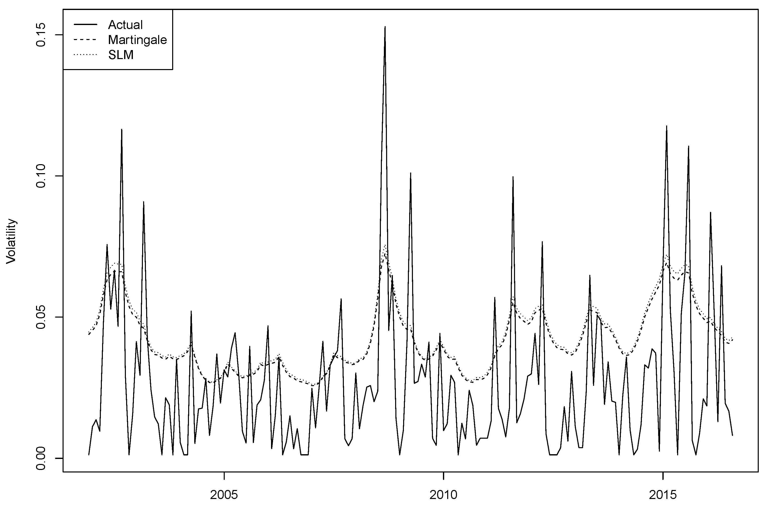
reports WAIC and LOO information criteria for the unrestricted, $p\in [0,\infty )$, and restricted, $p\in [0.5,1.5]$ models. Imposing SLM does not worsen out of sample forecast behavior, as both WAIC and LOO attribute a smaller information criterion to the restricted model. Figure 9 plots fitted versus realized Focus volatility for both models in Table 7.

6. Discussion

Although one must recognize methodological choices and statistical uncertainty, we view the results of Section 4 and Section 5 as evidence that Focus survey forecasts are better characterized by a strict local martingale than a driftless true martingale process, specially through the first subsample from 2000/08 to 2008/07.

The nonparametric approach of empirically evaluating condition (3) is fundamentally limited by the range of observed values $S_t$ in a given time interval. We are trying to extrapolate from a compact set of $R_{+}$ properties of ${\sigma }^2\left(S_t\right)$ for all of $R_{+}$, and, as discussed in Jarrow et al. [7] results will invariably depend on the extension method employed.

Theorem 2 gives us empirically testable objective criteria that characterize a price process $S_t$ as either a true martingale or a strict local martingale. But formally estimating Heston-type models is not standard practice for understandable reasons. Classical likelihood inference has major difficulties when dealing with latent variables, what makes Bayesian simulation methods appealing.

When we compromise and fix $\lambda =1$, our estimates are still inconclusive with respect to Theorem 2—because although one can say with reasonable certainty that $\rho$ is positive, the posterior of p attributes significant probability to the true martingale range, what makes a more formal test of the strict local martingale hypothesis warranted.

We draw from developments in Bayesian model selection (Vehtari et al. [29]) and devise an experiment in which one imposes that $S_t$ is a strict local martingale (i.e., $\rho >0$ and $0.5<p<1.5$), and evaluate whether this restriction hinders out-of-sample forecast performance. Imposing SLM behavior does not worsen the out-of-sample forecast, but it is hard to distinguish between models. In hindsight this result is not surprising because even in the p-unrestricted model more, probability is attributed to the SLM range of $p\in (0.5,1.5)$ than otherwise.

7. Concluding Remarks

We investigate the puzzling poor performance of Brazilian market participants in forecasting the BRL-USD exchange rate. Extrapolations of forward rates are a better predictor of the 30-days ahead spot exchange rates than Focus survey forecasts—which are also biased through a substantial portion of our sample, from August 2002 to July 2007. This result is counter-intuitive since Focus participants have access to the information on the future foreign exchange market, and yet they make biased forecasts.

Dandapani and Protter [1] describe a mechanism through which the incorporation of new information induces a drift in an otherwise driftless local martingale, turning it into a strict local martingale. We argue this filtration enlargement mechanism could help explain our forecast performance conundrum. Spot and future rates are consistent with martingales, while Focus forecasts have a bias term, equivalent to the presence of a drift. Another important feature is the presence of stochastic volatility in this process, important in the characterization of a strict local martingale used by Dandapani and Protter [1] to represent the drift term generated by the process of information acquisition (filtration enlargement).

In order to investigate the strict local martingale hypothesis, we employ two different identification methods. The first one is a nonparametric estimation of variance function ${\sigma }^2\left(S_t\right)$ and rely on condition (3)—that asserts a local martingale is a strict local martingale if its volatility increases faster than linearly with level. Focus forecasts are less volatile, in absolute terms, than either spot or future rates, but Focus volatility increases faster for higher price observations. The second draws on results of Andersen and Piterbarg [25]: depending on parameter values of the stochastic volatility model (13), the underlying price process is either a true martingale or a strict local martingale. Employing Bayesian simulation techniques we estimate Focus 30-days ahead exchange rate forecasts follow a strict local martingale with higher probability than otherwise.

In this paper we present a new way of interpreting the presence of biased forecasts in a market where there are alternative forecasting methods that are informationally efficient. Using the filtering process proposed by Dandapani and Protter [1], we show that in the presence of stochastic volatility it is possible that more informed forecasts are worse than predictions based on a set of more restricted information. This result is important for the analysis of learning processes and information acquisition in financial markets.