1. Introduction
Misclassifications can occur in binomial data due to human errors or imprecise diagnostic procedures. Typically, misclassifications of both types (false-positive or false-negative) are possible. In a one-sample case, for instance, with an imperfect blood test, a healthy patient can be mistakenly classified as sick and vice versa. However, in some cases, only one type of misclassification exists. For example, Moors et al. [
1] presented auditing data where only false-negative (under-reported) errors occurred. Perry et al. [
2] showed blood testing data which had only false-positive (over-reported) errors. In a two-sample case, for example, we may wish to obtain the odds ratio for lung cancer (or traffic accidents) between males and females. The grouping variables (males/females) can typically be inerrant while the response variable (cancer/not) can sometime be misclassified (errant). In this lung cancer (two-sample) case, under-reporting (false-negative) occurs when a person (male/female) dies due to lung cancer but this fact is not reflected in the death certificate. As another example, in the traffic accident case, over-reporting (false-positive) occurs when a driver has lied to a police officer about not wearing a seatbelt, while the hospital record examination showed otherwise, for an example see the U.S. National Highway Traffic Safety Administration, NHTSA [
3].
Among many researchers, Bross [
4] reported that classical estimators ignoring misclassification can be extremely biased for certain applications.
Due to economic viability reasons, in some cases, the binary outcome variable can be obtained using an errant classifier/device. In such cases, classical inferential methods are testing and estimating proportion parameters corresponding to the errant classifier/device, but not to an inerrant device (gold standard). As a consequence, these classical methods are biased and invalid. For example, Tenenbein [
5] derived a formula quantifying the bias of the classical estimator of a single proportion in misclassified binomial data. Therefore, such misclassified binomial data need to be somehow augmented to make valid statistical inferences on the proportion parameters corresponding to the inerrant device.
The most frequently used data-augmenting method for misclassified binomial data is the double-sampling scheme, pioneered by Tenenbein [
5] for the one-sample problem. Such a scheme assumes an inerrant device is available only to a small number of experimental units due to economic viability reasons. The double-sampling scheme works in the following way. First, either a random subsample from the original misclassified data or another new sample is chosen. In the first case, where a random subsample from the original data is selected, we use the inerrant device to obtain the inerrant measurement of the binary outcome variable for the subsample. In the second case, where another new sample is selected, we use both the errant and the inerrant devices to obtain the binary outcome variable for this new sample. In both cases, we name the sample classified using only the errant device for the binary outcome variable as the original study and the sample classified using both the errant and inerrant devices for the binary outcome variable as the validation sub-study. Statistical inference is made based on the augmented overall data, combining the original study and the validation sub-study.
The following is the literature regarding several statistical inference methods for one-sample and two-sample misclassified binomial data. For one-sample data with only one type of misclassification error (false-positive or false-negative error), Moors et al. [
1] derived a one-sided exact confidence interval (CI) and Boese et al. [
6] derived several likelihood-based confidence intervals for the proportion parameters corresponding to the inerrant device (the true proportion parameter). Raats and Moors [
7] and Lee and Byun [
8] reported Bayesian credible intervals for the true proportion parameter with one type of misclassification only. For one-sample data with both types of misclassification errors, Raats and Moors [
7] derived both an exact confidence interval and a Bayesian credible interval for the true proportion parameter, and Lee [
9] reported a Bayesian interval estimation for the true binomial proportion parameter. For two-sample data with two types of misclassification errors, Prescott and Garthwaite [
10] proposed a Bayesian credible interval, and Morrissey and Spiegelman [
11] derived likelihood-based confidence intervals for the odds ratio. However, their methods are computationally burdensome, not guaranteed to converge to the true parameter value, and hard to reproduce by other practitioners.
In this paper we dealt with two-sample binomial data with one type of misclassification error obtained using double sampling, via a Bayesian approach. Our research objectives are to conduct Bayesian inference for the difference of two proportion parameters in over-reported two-sample binomial data using the doubly sample. The remainder of the paper is organized as follows. In
Section 2 we describe the data. In
Section 3 we develop a Bayesian point and interval estimation. Next, we illustrate our Bayesian method using real data, in
Section 4. A discussion follows in
Section 5.
2. Data
In this section, we consider doubly-sampled data containing two samples in both the original study and the validation sub-study subject to one type of misclassification error. Without loss of generality (WLOG), we assume that the data were obtained using an errant classification procedure that yields false-positive but not false-negative counts. For sample i (i = 1, 2), we let mi and ni be the number of items in the original and the validation study, respectively. We then defined Ni = mi + ni as the total sample size for Sample i. For the jth item in the ith sample, where i = 1, 2, and j = 1, …, Ni, we let Fij and Tij be the binary response variables obtained by the errant and inerrant devices, respectively. Next, we denote Fij = 1 if the result is positive by the errant device and Fij = 0 otherwise. The binary variable Tij is similarly defined for the inerrant device. Note that Fij is observed for all items in both the original study and the validation sub-study, while Tij is observed for items in the validation sub-study but not for items in the original study. Clearly, misclassification error occurs when Fij differs from Tij.
In the validation sub-study, for
i = 1, 2,
j = 0, 1, and
k = 0, 1, we use
nijk to denote the number of items in Sample
i classified as
j and
k by the inerrant device and the errant device, respectively. In the main study, we let
xi and
yi be the number of positive and negative classifications in Sample
i obtained by the errant device. The summary frequencies in both the main study and the validation sub-study for sample
i are displayed in
Table 1.
Next, we define the parameters for sample
i as follows. We let the true proportion parameter of interest be
, the proportion parameter of the errant device be
, and the false-positive rate of the errant device be
. Note that
πi is not an additional unique parameter because it is obtainable by using all other parameters. In particular, by the law of total probability, we have
where
qi = 1 −
pi. For the summary frequencies displayed in
Table 1, the corresponding cell probabilities are shown in
Table 2.
Our goal is to conduct Bayesian inference and we are interested in estimating and testing if a difference exists among the two true proportion parameters
In particular, the statistical hypotheses are
We develop Bayesian algorithms to estimate all the parameters in Expression (1) and constructed a Bayesian credible interval (CI) to see whether the two true proportion parameters
are equal (i.e., if zero is in the CI). We note that the proportion difference,
can be expressed as follows:
Therefore, our objective is ultimately to construct a 100(1 − α)% Bayesian CI for and hence, simultaneously test (2) by checking if zero is in the 100(1 − α)% Bayesian CI for , where α is the type-I error rate.
3. Model
We derive the Bayesian inference for the data described in the previous section. Specifically, we develop a closed-form algorithm for sampling from the exact joint posterior distribution of all the parameters given the data. Once a posterior sample is drawn for p1 and p2 then a posterior sample for the difference, in Expression (3) can be obtained. Finally, we construct a 100(1–α)% CI for
WLOG, for Sample
i in
Table 1, the observed counts (
ni00,
ni01,
ni11) of the validation sub-study have a trinomial distribution with total size
ni and probabilities displayed in an upper right 2 × 2 submatrix in
Table 2, i.e.,
In addition, the observed counts
in the main study have the following binomial distribution:
Since
and
are independent for group
i and these cell counts are independent across groups, the sampling distribution of the vector of all data
given the vector of all parameters
is
To put it into a Bayesian framework, a non-informative proper prior for
is chosen. In particular, a uniform prior for each component of
is chosen, where each parameter (i.e., component of
) is constrained to lay in an interval of (0, 1), and we assume that these priors are independent, i.e., the joint prior distribution is
The following reasons explain why the uniform priors are chosen. First, typically in most applications, the prior information is unknown (non-informative); therefore, a uniform prior which is a special case of Beta distribution, i.e., Beta (1, 1) equivalence, would be appropriate since the distribution is flat or constant (non-informative) for all possible values within (0, 1) interval constraints. Second, the availability of the validation sub-study provides information about all model parameters and therefore an informative prior is not needed any more. Third, as Yang and Berger [
12] mentioned, Bayesian analysis with non-informative priors is increasingly recognized as a method for classical statisticians to obtain good classical procedures. In this paper, it is also desirable to aim for such a frequentist matching approach to develop non-informative (flat or constant) priors (i.e., most suitably, uniform priors) to ensure that we have Bayesian credible sets with good/matching frequentist properties for our forthcoming future research so as to find good/matching frequentist confidence intervals.
Combining Equations (7) and (8), we obtain the following joint posterior distribution:
which has the same functional form as the sampling distribution in Equation (7).
In general, it is nontrivial to sample from the posterior distribution (9). Therefore, we derive a closed-form algorithm for sampling from Equation (9) via the reparameterization of
. Note that the term reparameterization is different than transformation. For transformation a Jacobian is needed, while in reparameterization we simply reparametrize the original parameters for algebraic convenience and hence, no Jacobian is needed. Note also that other non-informative priors than the uniform prior, such as Beta (½, ½) which is the Jeffreys prior, could also be considered plausible or sensible (depending on the specific aim of the problem statement), as long as they produce proper posteriors and as long as they are in alignment with desirable good/matching frequentist properties, resulting in a good/matching frequentist likelihood function for its corresponding/counterpart frequentist confidence intervals. Also note that proper means it is a probability density and hence does integrate to 1, while improper means it is not a probability density and hence does not integrate to 1. In particular, we define
Using Equation (10), the posterior density in Equation (9) become
where
d is defined in Equation (6) and
is the re-parameterized parameter vector. Because the re-parameterized parameter vector of Equation (12) is now separable, we can straightforwardly draw
from the posterior Equation (11) by using the following closed-form algorithm:
with
Next, when
are available, we can obtain
by solving Equations (1) and (10) so that
In summary, the following is the closed-form algorithm to sample from the posterior density of Equation (11).
Choose a large number J, say, 10,000, as a large sample size for the posterior draw.
Obtain J samples of , each for using (13) and (14), respectively.
Obtain J samples of , each for using (15) and (16), respectively.
Compute J samples of each difference, from Equation (3).
Use the median of the posterior sample of as a point estimator of The median was chosen because the distribution of the posterior sample of is skewed.
Obtain a 100(1–α)% CI for by using the lower and upper (α/2)th percentile of the sample of where α is the type I error rate.
Finally, the statistical hypothesis testing in (2) can be rejected if this CI does not contain the number zero.
4. Example
As an illustration of our proposed procedure, we utilize over-a-decade old retrospective data collected from a large introductory statistics class (1148 students) at a university in the United States of America. This is not a prospective study with randomized trials. Several teaching assistants (TA) were hired to grade the homework, quizzes, extra credits, etc. from the laboratory (lab) component of that course. Note that to alleviate extremely high volumes for homework grading, only two selected problems were chosen to be graded, but these were not pre-announced to the students. Hence, the students were still required to do all assigned homework problems. Grades in this lab portion of the course constituted only 20% of the course grade. Due to the large class size, weekly time constraints, and the need for speed grading so that assignments could be returned in a timely manner, the TA (errant device) tended to grade assignments on a pass/fail scale very leniently to avoid students coming back to bargain for better scores. This resulted in an overly high pass rate, i.e., a false-positive rate for the lab portion of the course grade. In that lab portion of the course grade, “pass” was defined as 60% or above, and was coded as 1 (
Table 1,
Table 2 and
Table 3). Likewise, “fail” was defined as below 60% and was coded as 0. The professor (inerrant device) was interested in auditing those TAs’ grading for the quality of graded (pass/fail) lab scores. He randomly selected a smaller sample of size 434 (144 + 23 + 47 + 169 + 13 + 38) as a validation sub-study. This total validation sub-study size, 434 out of 1148 (37.8%), is not small. As the professor’s original intention was to draw validation samples until a sufficient number of false-positive errors were caught, he convinced himself that this kind of grading system is sustainable in the long run for many large classes. It turns out that he caught 13 out of 582 (about 2%) of false-positive errors in the female group and 23 out of 656 (about 4%) in the male groups. Both group’s error rates were satisfactory for the professor’s original intention.
In this study, the interest is to estimate the overall score/performance of male and female students, in terms of their proportion difference. Summary statistics of data are provided in
Table 3.
Note that, since there is no personally identifiable information (PII) of any human subject (such as the person’s name, university name, date of birth or DOB, social security number or SSN, numeric grades, etc.) involved, and only summary statistics (such as counts and proportions of pass/fail lab portion, in
Table 3) are displayed, an International Review Board (IRB) approval or an exemption to collect such data and publish results based on
Table 3 is not required. Moreover, this was a student class assignment which was a sole exception for classroom activities, and hence did not fall under the jurisdiction of the IRB and did not require IRB application, approval, or oversight (
http://research-compliance.umich.edu/human-subjects/human-research-protection-program-hrpp/hrpp-policies/class-assignments-irb-approval).
From Expression (2), the null hypothesis in this context is to test if the proportions of failing the lab portion of the course between male and female students are the same, i.e., the
in Expression (3) is equal to zero; with the alternative hypothesis that the two proportions are not the same, i.e.,
is not equal to zero. Following the algorithm from the previous section, the median of the posterior sampling distribution of the proportion difference
is 0.024, i.e., the proportion difference of failing the course for male students is about 0.024 points more than female students, i.e., we see that the male students had about a 2.4% higher chance of failing the lab portion of the course than female students. The resulting 90% Bayesian CI for the difference
is (−0.014, 0.063). Because this CI contains zero, we conclude that the study did not provide enough statistical evidence in support of the outcome (pass/fail) difference between the two genders (male/female students).
Table 4 displays the parameter estimates and 90% CI for the audited pass/fail data.
5. Simulation
We conduct simulation studies to evaluate and compare the performance of our algorithms under various scenarios, such as evaluating the impact on the CIs of by varying sample sizes, the ratio of validation and original study, and the false-positive rate. We considered a two-sided nominal type-I error level of α = 0.1. Although not required by our algorithm, in order to simplify the conduct of the simulation studies and the presentation of the simulation results, we let the total sample sizes be N1 = N2 = N, sub-study sample sizes be n1 = n2 = n, and false-positive rates be φ1 = φ2 = φ. For each simulation scenario a total of K = 10,000 datasets is generated.
We consider 32 simulation scenarios resulting from combinations of the following values:
True proportion parameters of interest
False-positive rate φ = 0.1, 0.2.
Ratio of sub-study sample size versus the total sample size r = n/N = 0.2, 0.4.
Total sample size N = 100, 200, 300, 400.
For each simulation scenario, we simulate
K = 10,000 datasets. Within each dataset, we draw a size of
J = 10,000 posterior samples of
according to the algorithm in
Section 3. We then compute the posterior median (point estimator) and a 90% CI. Finally, we generate boxplots of the
K posterior medians of
to examine their behavior around the true
In addition, we calculate the coverage probability (CP) and the average length (AL) of the
K CIs.
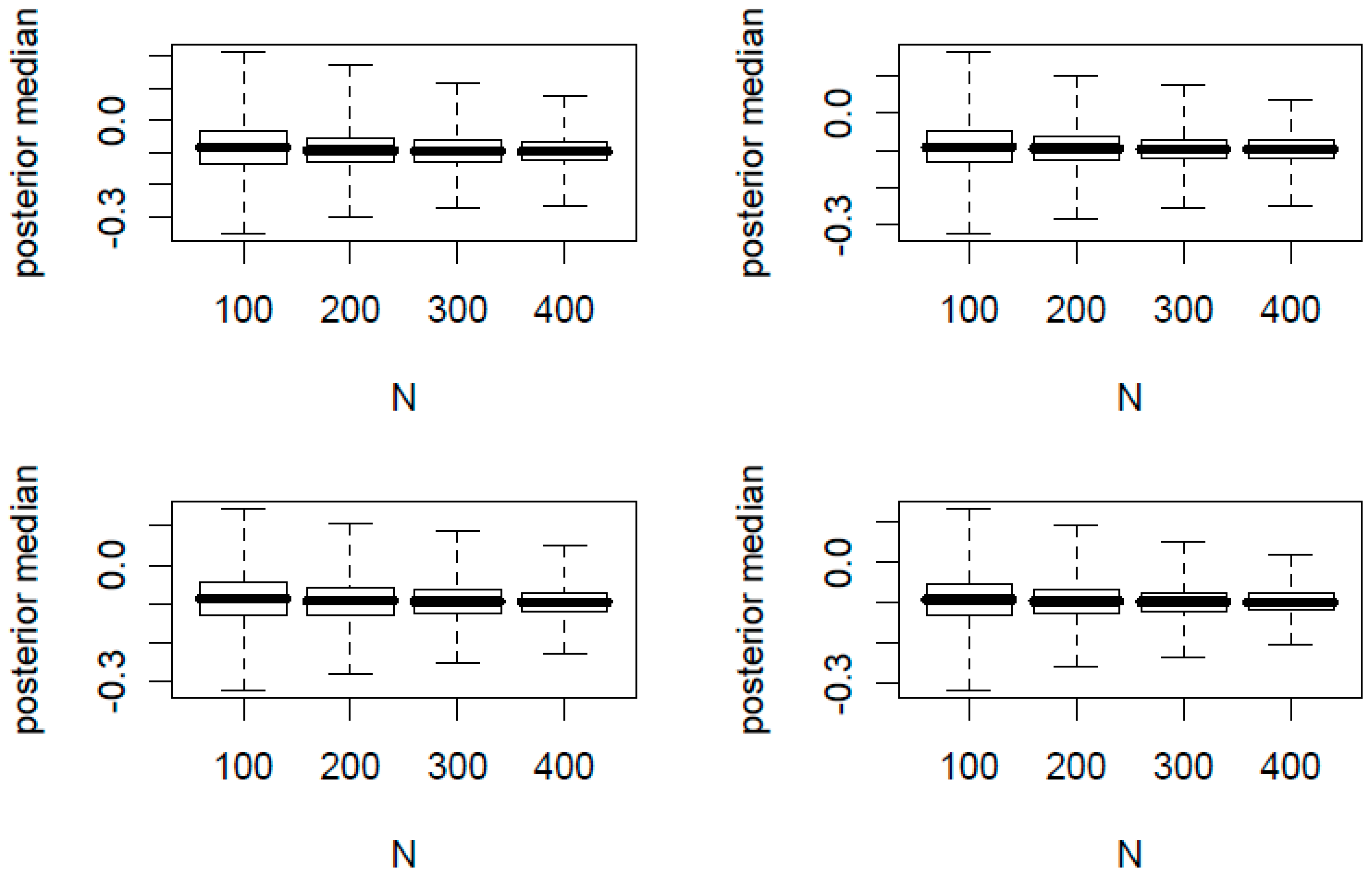
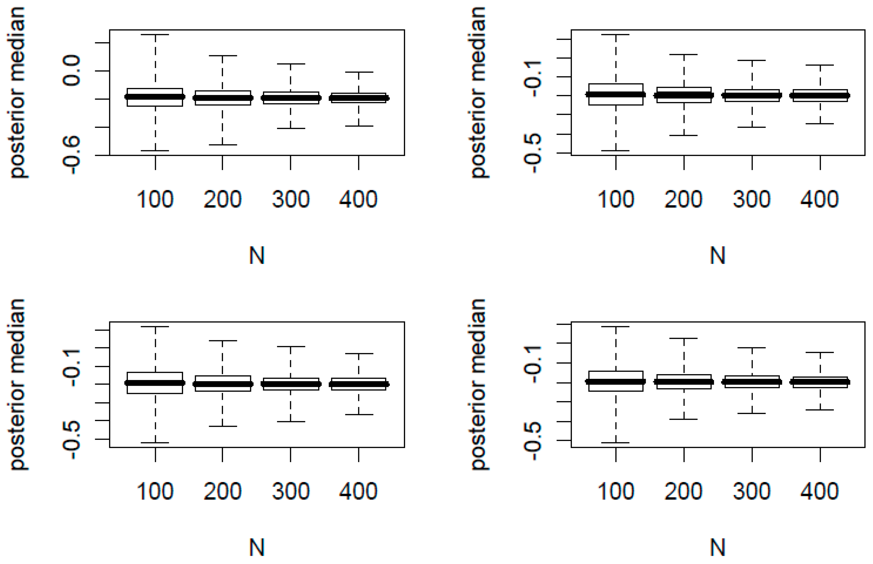
In
Figure 1 and
Figure 2, we present the boxplots of
K posterior medians of
against the total sample size
N. The true proportion parameters of
are (0.1, 0.2) and (0.4, 0.6) for
Figure 1 and
Figure 2, respectively. In each figure, the top two panels have
φ = 0.2 and the bottom two panels have
φ = 0.1. In addition, the left two panels have
n/
N = 0.2 and the right two panels have
n/
N = 0.4.
From the 32 simulation scenarios for both figures, the posterior medians are centered around the true and hence is a good point estimator. Additionally we made the following observations:
For each panel of four boxplots, the variation of the posterior medians decreases as N increases.
For each figure, the variation of the posterior medians of the top two panels with a larger φ is slightly greater than that of the bottom two panels with a smaller φ.
For each figure, the variation of the posterior medians of the left two panels with a smaller n/N is slightly greater than that of the right two panels with a larger n/N.
In
Table 5, we show the CPs and ALs of the
K CIs of
for each simulation scenario. Since the CPs are all close to the nominal 90% level, this is an indication that our CI estimator is a good estimator. Similar to the observations made for the figures, we made the following observations in
Table 5:
For fixed , φ, n/N, the AL of the CIs decreases as N increases.
For fixed , n/N, N, the AL of the CIs decreases as φ decreases.
For fixed , φ, N, the AL of the CIs decreases as n/N increases.
6. Discussion
In this article we derived a Bayesian algorithm to conduct statistical inference on the difference of two proportion parameters for binary data subject to one type of misclassification. Our closed-form algorithm to draw from the full posterior distributions has many advantages, including the following:
Since we draw directly from the posterior distributions, there is no need to specify initial values and there is no burn-in period or convergence problem.
Our algorithm can handle zero counts as shown in Equations (13) and (14).
No asymptotic (large sample) theory is involved and hence it is easy to implement, in the sense that our algorithm does not require a large sample size for the complex asymptotic (large sample) theory, such as the regularity conditions, to work out—rather, it simply draws from the joint posterior distribution.
The uniform (0, 1) prior distribution in Equation (8) is identical to a Beta (1, 1) distribution; however, to generalize this prior distribution in Expression (8) to be Beta (α, β) would complicate Equations (8) and (9). This would affect the generalized sensibility of the results in relation to the choice of the hyper-parameter values. Still, doing so can be considered so long as the hyper-parameter choices produce sensible proper (i.e., a probability density that integrates to 1) posteriors and produce the corresponding good/matching frequentist’s counterpart of confidence intervals. For example, the Uniform (0, 1) priors which are Beta (1, 1) and the Jeffreys priors which are Beta (½, ½) satisfy the above two aforementioned criteria.

