A Support Vector Machine Based Approach for Predicting the Risk of Freshwater Disease Emergence in England

 ,
, 


Abstract
:1. Introduction
2. Data
3. Methodology
3.1. Classification of Disease Emergence Risk
- The native and non-native fish movements into a cell increases the diversity of fish species in a cell.
- The diversity of fish in a cell contributes towards the likelihood of one of fish holding a pathogen. That is, the more varied the more likely they are to hold a pathogen.
- The higher is the number of fish movements into a cell, the higher is the possibility of a freshwater fish disease emerging in that cell.
3.2. Support Vector Machine (SVM)
- Linear Kernel: .
- dth-Degree polynomial: .
- Gaussian: .
- Radial basis: .
- Neural network: .
4. Empirical Results
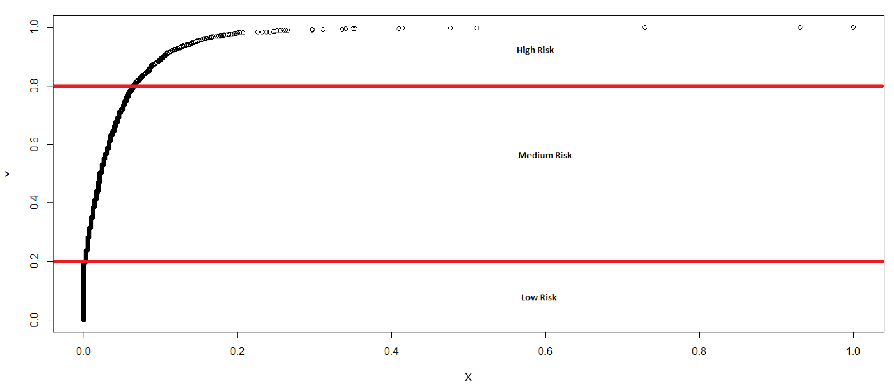
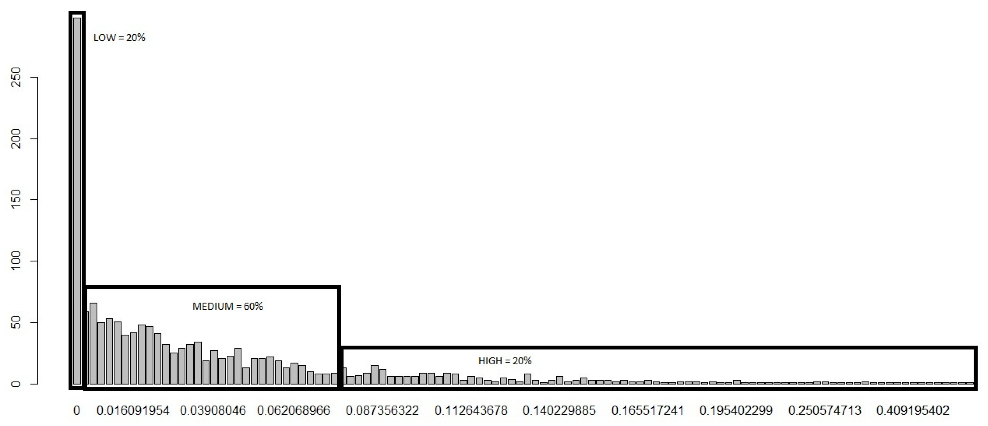
4.1. Risk Classification
- The risk of disease emergence is categorized as low where each cell in the dataset for which the corresponding “Sum” and No. of Varieties equal zero.
- The risk is classified as medium when each cell in the dataset records a “Sum” greater than or equal to one and less than or equal to 28, in addition to the corresponding No. of Varieties equalling zero.
- The risk categorization is high when each cell in the dataset records a “Sum” greater than 28 and the No. of Varieties greater than or equal to zero. We categorize using the greater than or equal to sign for High risk because it appears reasonable (based on initial assumptions and expert opinions) to conclude that, even if the No. of Varieties equal zero, if the “Sum” is greater than 28, the movement of fish into that cell is statistically large enough (based on our c.d.f) for us to expect a high risk of disease emergence.
4.2. Output from the Proposed SVM Model
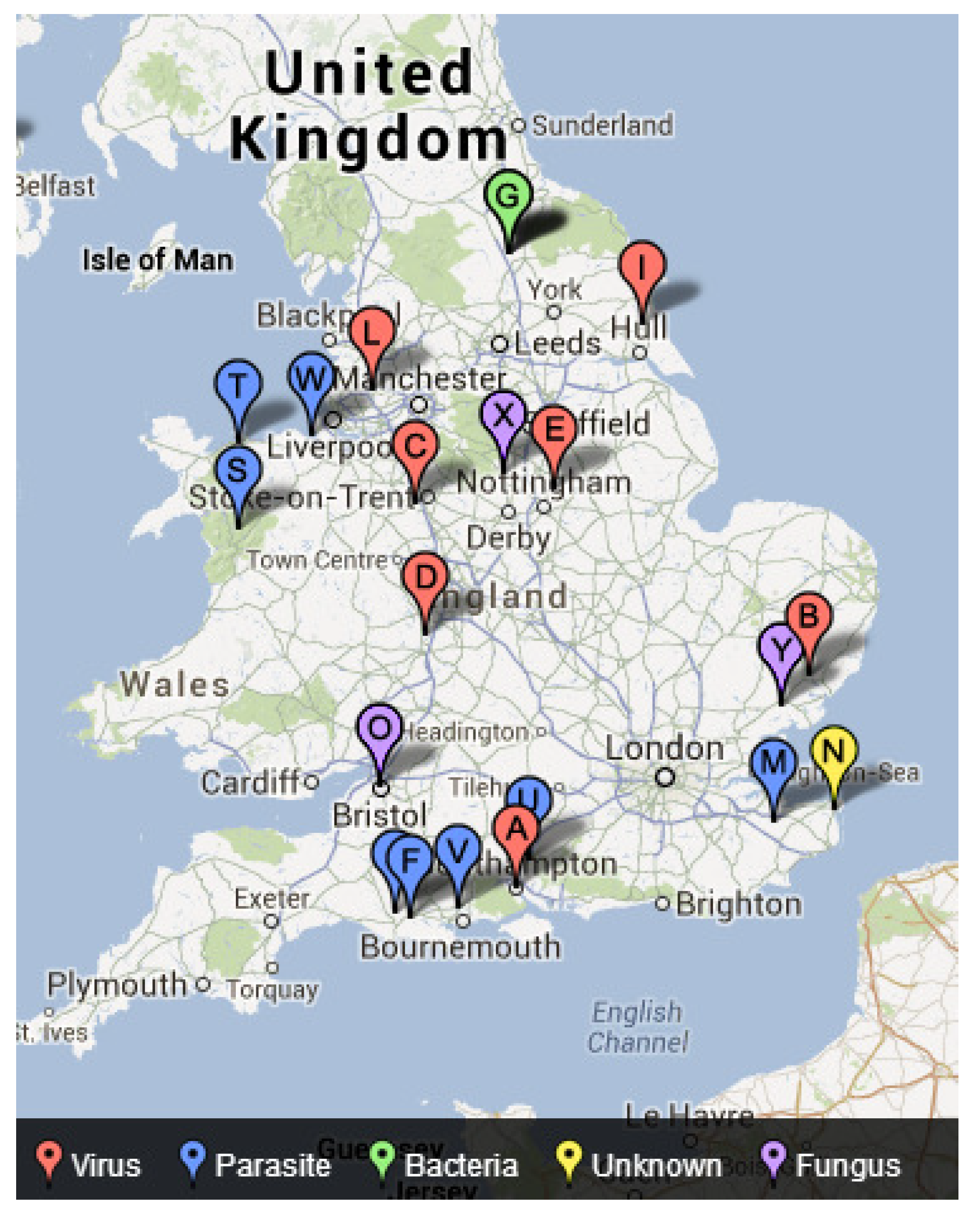
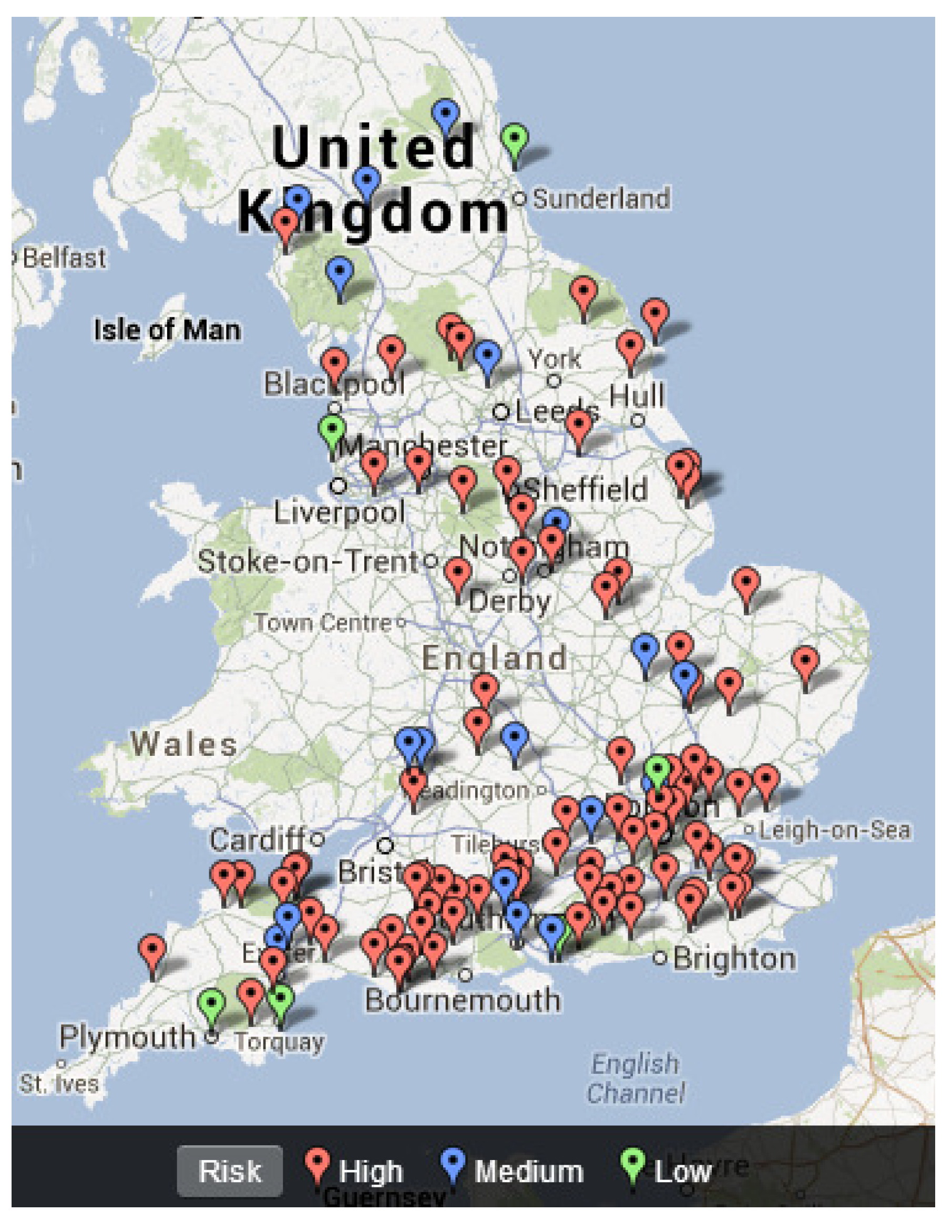
4.3. Mapping Freshwater Disease Emergence in England
5. Conclusions
Author Contributions
Funding
Acknowledgments
Conflicts of Interest
References
- Raptis, C.E.; van Vliet, M.T.H.; Pfister, S. Global thermal pollution of rivers from thermoelectric power plants. Environ. Res. Lett. 2017, 11, 104011. [Google Scholar] [CrossRef]
- Shen, Y.; Cao, H.; Tang, M.; Deng, H. The Human Threat to River Ecosystems at the Watershed Scale: An Ecological Security Assessment of the Songhua River Basin, Northeast China. Water 2017, 9, 219. [Google Scholar] [CrossRef]
- Wen, Y.; Schoups, G.; van de Giesen, N. Organic pollution of rivers: Combined threats of urbanization, livestock farming and global climate change. Sci. Rep. 2017, 7, 43289. Available online: https://www.nature.com/articles/srep43289 (accessed on 21 August 2018). [CrossRef] [PubMed]
- Crist, E.; Mora, C.; Engelman, R. The interaction of human population, food production, and biodiversity protection. Science 2017, 356, 260–264. [Google Scholar] [CrossRef] [PubMed]
- Vorosmarty, C.J.; McIntyre, P.B.; Gessner, M.O.; Dudgeon, D.; Prusevich, A.; Green, P.; Glidden, S.; Bunn, S.E.; Sullivan, A.; Reidy Liermann, C.; et al. Global threats to human water security and river biodiversity. Nature 2010, 467, 555–561. [Google Scholar] [CrossRef] [PubMed]
- Cortes, C.; Vapnik, V. Support Vector Machines. Mach. Learn. 1995, 20, 273–297. [Google Scholar] [CrossRef]
- Vapnik, V. The Nature of Statistical Learning Theory; Springer: New York, NY, USA, 1995. [Google Scholar]
- Auria, L.; Moro, R.A. Support Vector Machines (SVM) as a Technique for Solvency Analysis; Technical Report; Deutsche Bundesbank: Hannover, Germany; German Institute for Economic Research: Berlin, Germany, 2008; Available online: https://papers.ssrn.com/sol3/papers.cfm?abstract_id=1424949 (accessed on 21 August 2018).
- Xie, Z.; Lou, I.; Ung, W.K.; Mok, K.M. Freshwater Algal Bloom Prediction by Support Vector Machine in Macau Storage Reservoirs. Math. Prob. Eng. 2012, 2012, 397473. Available online: https://www.hindawi.com/journals/mpe/2012/397473/ (accessed on 21 August 2018). [CrossRef]
- Son, Y.-J.; Kim, H.-G.; Kim, E.-H.; Choi, S.; Lee, S.-K. Application of Support Vector Machine for Prediction of Medication Adherence in Heart Failure Patients. Healthc. Inform. Res. 2010, 16, 253–259. [Google Scholar] [CrossRef] [PubMed]
- Nicolaou, N.; Georgiou, J. Detection of epileptic electroencephalogram based on Permutation Entropy and Support Vector Machines. Expert Syst. Appl. 2012, 39, 202–209. [Google Scholar] [CrossRef]
- Sun, J.; Li, H. Financial distress prediction using support vector machines: Ensemble vs. individual. Appl. Soft Comput. 2012, 12, 2254–2265. [Google Scholar] [CrossRef]
- Danenas, P.; Garsva, G. Selection of Support Vector Machines based classifiers for credit risk domain. Expert Syst. Appl. 2015, 42, 3194–3204. [Google Scholar] [CrossRef]
- Jiang, P.; Craig, P.; Crosky, A.; Maghrebi, M.; Canbulat, I.; Saydam, S. Risk assessment of failure of rock bolts in underground coal mines using support vector machines. Stat. Methods Min. Ind. 2018, 34, 293–304. [Google Scholar] [CrossRef]
- Zhou, Y.; Su, W.; Ding, L.; Luo, H. Predicting Safety Risks in Deep Foundation Pits in Subway Infrastructure Projects: Support Vector Machine Approach. J. Comput. Civ. Eng. 2017, 31. [Google Scholar] [CrossRef]
- Lin, K.-P.; Pai, P.-F.; Lu, Y.-M.; Chang, P.-T. Revenue forecasting using a least-squares support vector regression model in a fuzzy environment. Inf. Sci. 2013, 220, 196–209. [Google Scholar] [CrossRef]
- Santamaria-Bonfil, G.; Reyes-Ballesteros, A.; Gershenson, C. Wind speed forecasting for wind farms: A method based on support vector regression. Renew. Energy 2016, 85, 790–809. [Google Scholar] [CrossRef]
- Ebrahim, H.; Rajaee, T. Simulation of groundwater level variations using wavelet combined with neural network, linear regression and support vector machine. Glob. Planet. Chang. 2017, 148, 181–191. [Google Scholar] [CrossRef]
- Omrani, E.; Khoshnevisan, B.; Shamshirband, S.; Saboohi, H.; Anuar, N.B.; Nasir, M.H.N.M. Potential of radial basis function-based support vector regression for apple disease detection. Measurement 2014, 55, 512–519. [Google Scholar] [CrossRef]
- Lou, I.; Xie, Z.; Ung, W.K.; Mok, K.M. Integrating Support Vector Regression with Particle Swarm Optimization for numerical modeling for algal blooms of freshwater. Appl. Math. Model. 2015, 39, 5907–5916. [Google Scholar] [CrossRef]
- Lou, I.; Xie, Z.; Ung, W.K.; Mok, K.M. Integrating Support Vector Regression with Particle Swarm Optimization for Numerical Modeling for Algal Blooms of Freshwater. In Advances in Monitoring and Modelling Algal Blooms in Freshwater Reservoirs; Lou, I., Han, B., Zhang, W., Eds.; Springer: Dordrecht, The Netherlands, 2017. [Google Scholar]
- Wu, Y.; Yin, J.; Dai, Y.; Yuan, Y. Identification method of freshwater fish species using multi-kernel support vector machine with bee colony optimization. Trans. Chin. Soc. Agric. Eng. 2014, 30, 312–319. [Google Scholar]
- Park, Y.; Cho, K.H.; Park, J.; Cha, S.M.; Kim, J.H. Development of early-warning protocol for predicting chlorophyll-a concentration using machine learning models in freshwater and estuarine reservoirs, Korea. Sci. Total Environ. 2015, 502, 31–41. [Google Scholar] [CrossRef] [PubMed]
- Thrush, M.A.; Dunn, P.L.; Peeler, E.J. Monitoring Emerging Disease of Fish and Shellfish Using Electronic Sources. Transbound. Emerg. Dis. 2012, 59, 385–394. [Google Scholar] [CrossRef] [PubMed]
- Copp, G.H.; Vilizzi, L.; Gozlan, R.E. Fish Movements: The Introduction Pathway for Topmouth Gudgeon Pseudorasbora Parva and Other Non-Native Fishes in the UK. Aquat. Conserv. 2010, 20, 269–273. [Google Scholar] [CrossRef]
- Copp, G.H.; Vilizzi, L.; Gozlan, R.E. The demography of introduction pathways, propagule pressure and occurrences of non-native freshwater fish in England. Aquat. Conserv. 2010, 20, 595–601. [Google Scholar] [CrossRef]
- Ripley, B.D. Pattern Recognition and Neural Networks; Cambridge University Press: Cambridge, UK, 1996. [Google Scholar]
- Peeler, E.J.; Oidtmann, B.C.; Midtlyng, P.J.; Miossec, L.; Gozlan, R.E. Non-native aquatic animals introductions have driven disease emergence in Europe. Biol. Invasions 2011, 13, 1291–1303. [Google Scholar] [CrossRef]
- Vapnik, V. Statistical Learning Theory; Springer: New York, NY, USA, 1998. [Google Scholar]
- Brereton, R.G.; Lloyd, G.R. Support vector machines for classification and regression. Analyst 2010, 135, 230–267. [Google Scholar] [CrossRef] [PubMed]
- James, G.; Witten, D.; Hastie, T.; Tibshirani, R. An Introduction to Statistical Learning; Springer: New York, NY, USA, 2013. [Google Scholar]
- Hastie, T.; Tibshirani, R.; Friedman, J. The Elements of Statistical Learning: Data Mining, Inference, and Prediction; Springer: New York, NY, USA, 2009. [Google Scholar]
- Shannon, C. A Mathematical Theory of Communication. Bell Syst. Tech. J. 1948, 27, 379–423. [Google Scholar] [CrossRef]
- Hassani, H.; Dionisio, A.; Ghodsi, M. The effect of noise reduction in measuring the linear and nonlinear dependency of financial markets. Nonlinear Anal. Real World Appl. 2010, 11, 492–502. [Google Scholar] [CrossRef]
- Granger, G.; Lin, J. Using the mutual information coefficient to identify lags in nonlinear models. J. Time Ser. Anal. 1994, 15, 371–384. [Google Scholar] [CrossRef]

| Risk | Sum Variable | No. of Varieties |
|---|---|---|
| Low | 0 | 0 |
| Medium | ≤ 1 Sum ≤ 28 | 0 |
| High | Sum > 28 | ≥0 |
| Optimal Model | nu-svc | - | - |
|---|---|---|---|
| Training error | 2.80% | - | - |
| No. of support vectors | 521 | - | - |
| Parameter: nu | 0.2 | - | - |
| Hyperparameter: Sigma | 0.17869 | - | - |
| Objective Function Value | 11.4719 | 94.7225 | 483.1845 |
| 500 Iterations | Low Risk | Medium Risk | High Risk |
|---|---|---|---|
| Average Accuracy | 93.6% | 95.8% | 96.9% |
| Standard Deviation | 1.99% | 0.95% | 1.28% |
| CV for Accuracy | 213% | 98.6% | 132.58% |
| 100 Observations | Low | Medium | High |
|---|---|---|---|
| Accuracy | 90.0% | 91.0% | 94.0% |
| Standard Deviation | 3.02% | 1.96% | 2.17% |
| CV for Accuracy | 335% | 215% | 231% |
| Chi-Square | p-Value | |
|---|---|---|
| England | 4.858 | 0.088 * |
| City: | ||
| Southampton | 4.348 | 0.114 |
| Suffolk/Ipswich | 10.747 | 0.005 * |
| Staffordshire | 9.211 | 0.010 * |
| Worcestershire | 11.989 | 0.002 * |
| Nottinghamshire | 3.254 | 0.197 |
| Dorset | 7.471 | 0.024 * |
| North Yorkshire | 34.909 | 0.000 * |
| South & East | 1.338 | 0.512 |
| Eden | 17.815 | <0.001 * |
| Lancashire | 4.439 | 0.109 |
| North Kent | 6.849 | 0.033 * |
| Pegwell Bay, Kent | 0.119 | 0.942 |
| Bristol | 13.243 | 0.001 * |
| Northern Ireland | 2.814 | 0.245 |
| Mawddach, Wales | 1.2 | 0.549 |
| Lune | 4.487 | 0.106 |
| Tamar | 0.743 | 0.69 |
| Dee | 0.959 | 0.619 |
| Derbyshire | 3.55 | 0.17 |
| Colchester | 3.981 | 0.137 |
| Disease | Chi-Square | p-Value |
|---|---|---|
| Virus | 4.801 | 0.091 * |
| Bacteria | 6.116 | 0.047 * |
| Parasite | 1.446 | 0.485 |
| Fungus | 10.348 | 0.006 * |
| Unknown | 0.119 | 0.942 |
© 2019 by the authors. Licensee MDPI, Basel, Switzerland. This article is an open access article distributed under the terms and conditions of the Creative Commons Attribution (CC BY) license (http://creativecommons.org/licenses/by/4.0/).
Share and Cite
Hassani, H.; Silva, E.S.; Combe, M.; Andreou, D.; Ghodsi, M.; Yeganegi, M.R.; Gozlan, R.E. A Support Vector Machine Based Approach for Predicting the Risk of Freshwater Disease Emergence in England. Stats 2019, 2, 89-103. https://doi.org/10.3390/stats2010007
Hassani H, Silva ES, Combe M, Andreou D, Ghodsi M, Yeganegi MR, Gozlan RE. A Support Vector Machine Based Approach for Predicting the Risk of Freshwater Disease Emergence in England. Stats. 2019; 2(1):89-103. https://doi.org/10.3390/stats2010007
Chicago/Turabian StyleHassani, Hossein, Emmanuel S. Silva, Marine Combe, Demetra Andreou, Mansi Ghodsi, Mohammad Reza Yeganegi, and Rodolphe E. Gozlan. 2019. "A Support Vector Machine Based Approach for Predicting the Risk of Freshwater Disease Emergence in England" Stats 2, no. 1: 89-103. https://doi.org/10.3390/stats2010007
APA StyleHassani, H., Silva, E. S., Combe, M., Andreou, D., Ghodsi, M., Yeganegi, M. R., & Gozlan, R. E. (2019). A Support Vector Machine Based Approach for Predicting the Risk of Freshwater Disease Emergence in England. Stats, 2(1), 89-103. https://doi.org/10.3390/stats2010007