The Exponentiated Burr XII Power Series Distribution: Properties and Applications


Abstract
:1. Introduction and Motivation
2. Construction of the New Family
3. Special Sub Models
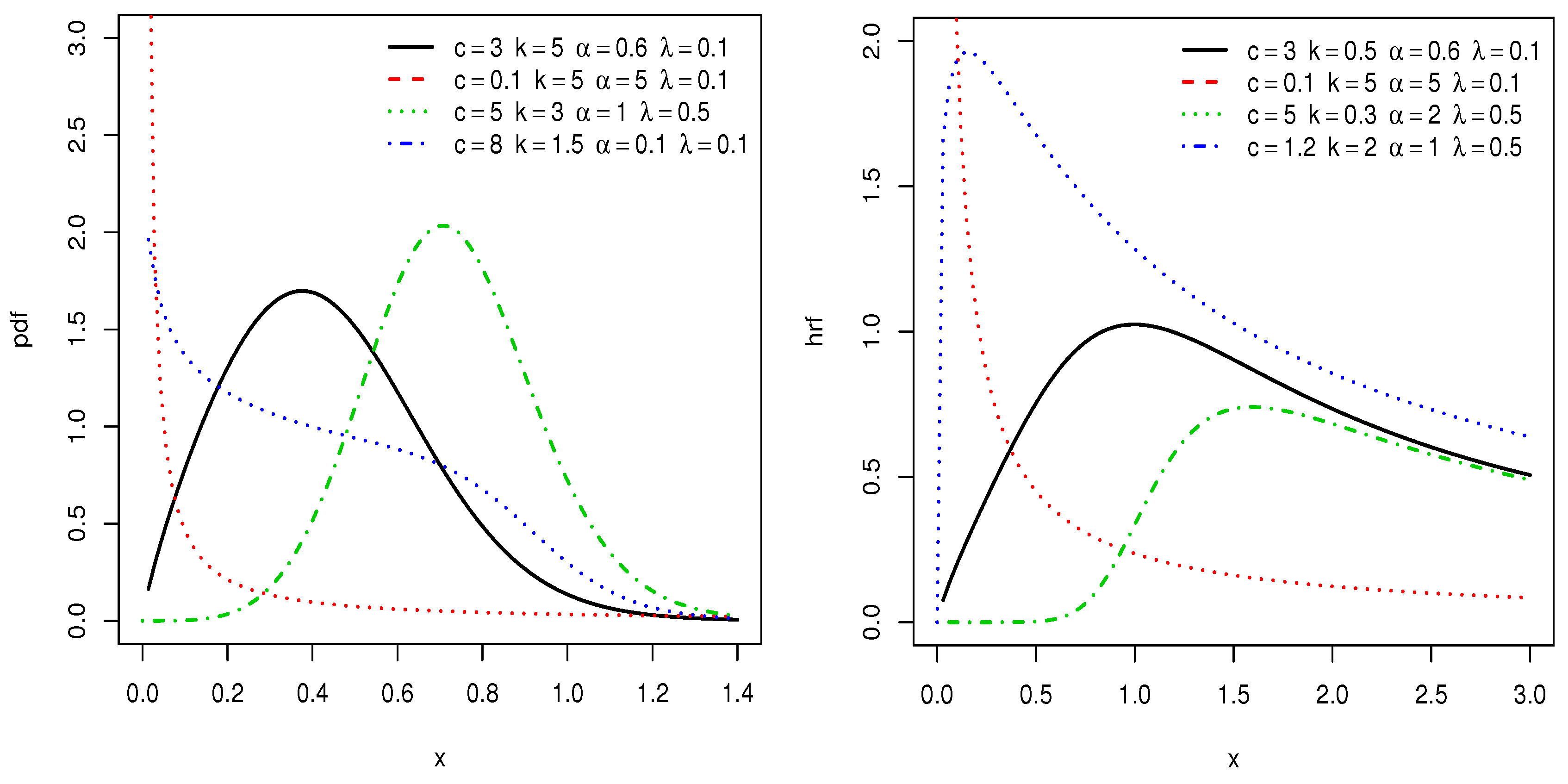
3.1. EBXII Logarithmic Distribution
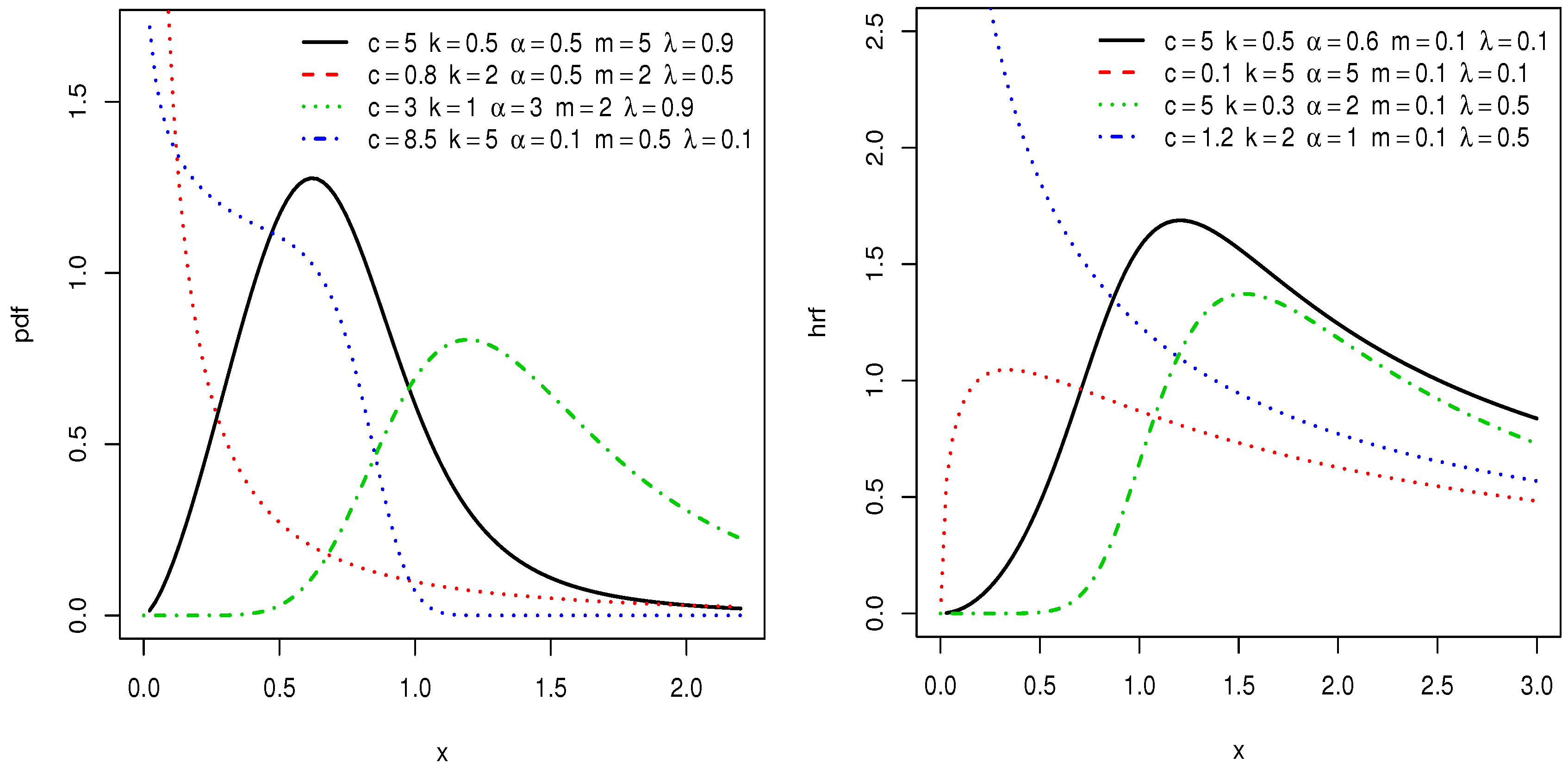
3.2. EBXII Binomial Distribution
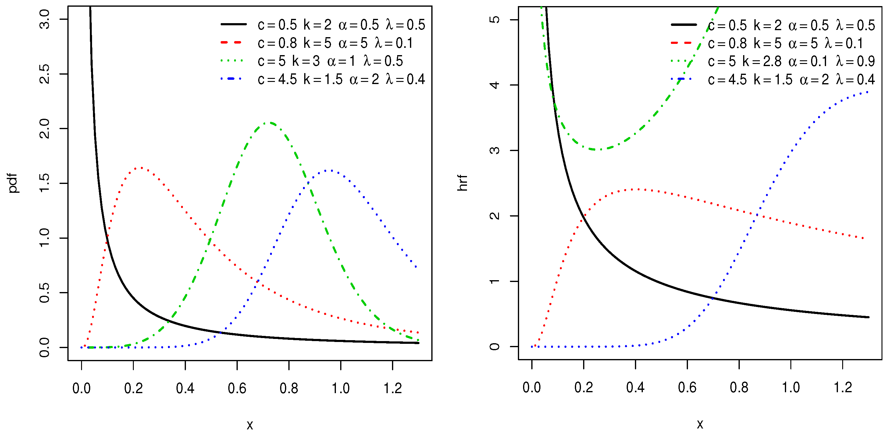
3.3. EBXII Poisson Distribution
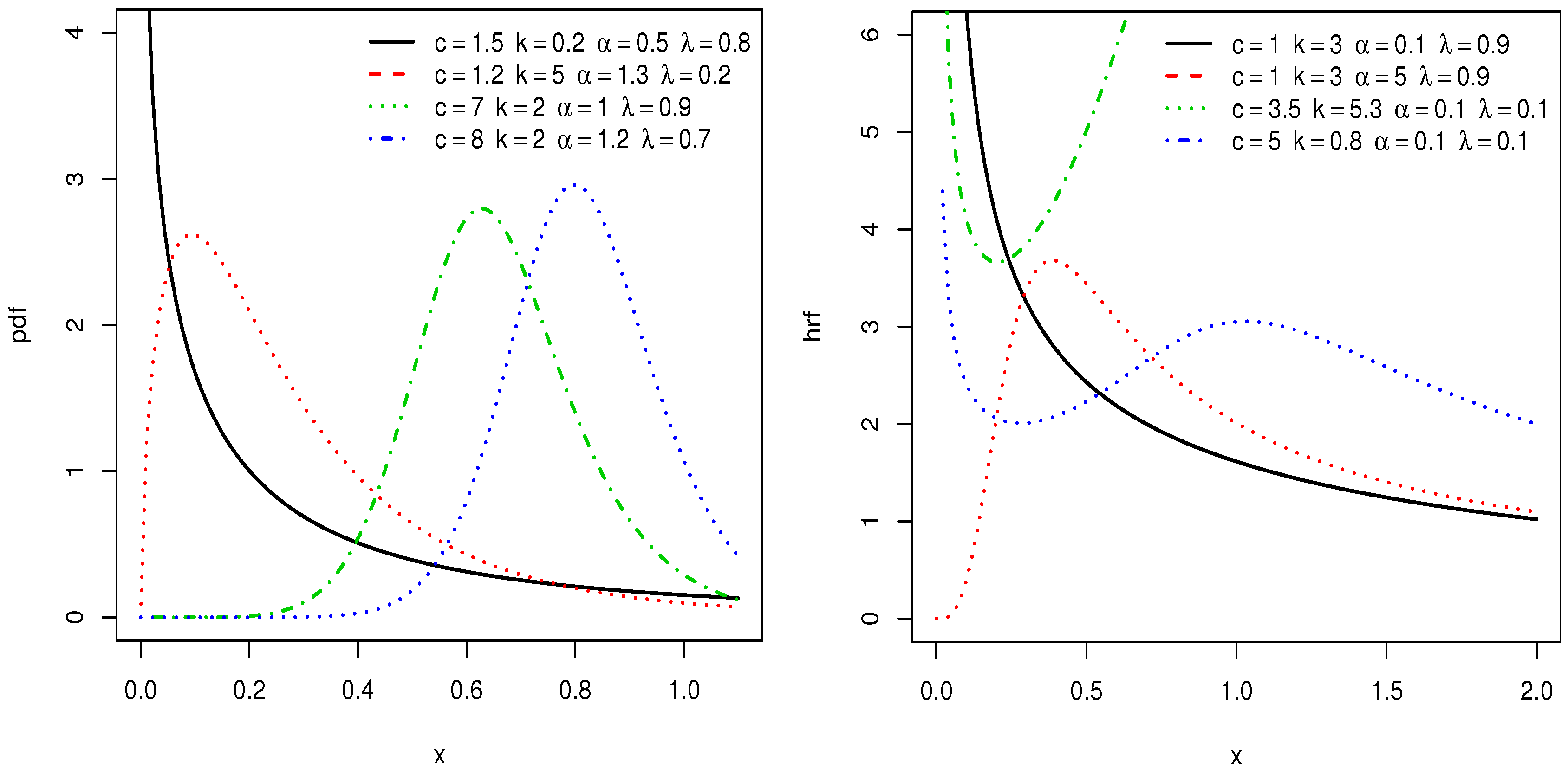
3.4. EBXII Geometric Distribution
4. Mathematical Properties
Moments
5. Estimation
6. Simulation Studies
- Generate
- Solve the following nonlinear equation for given parameters values,
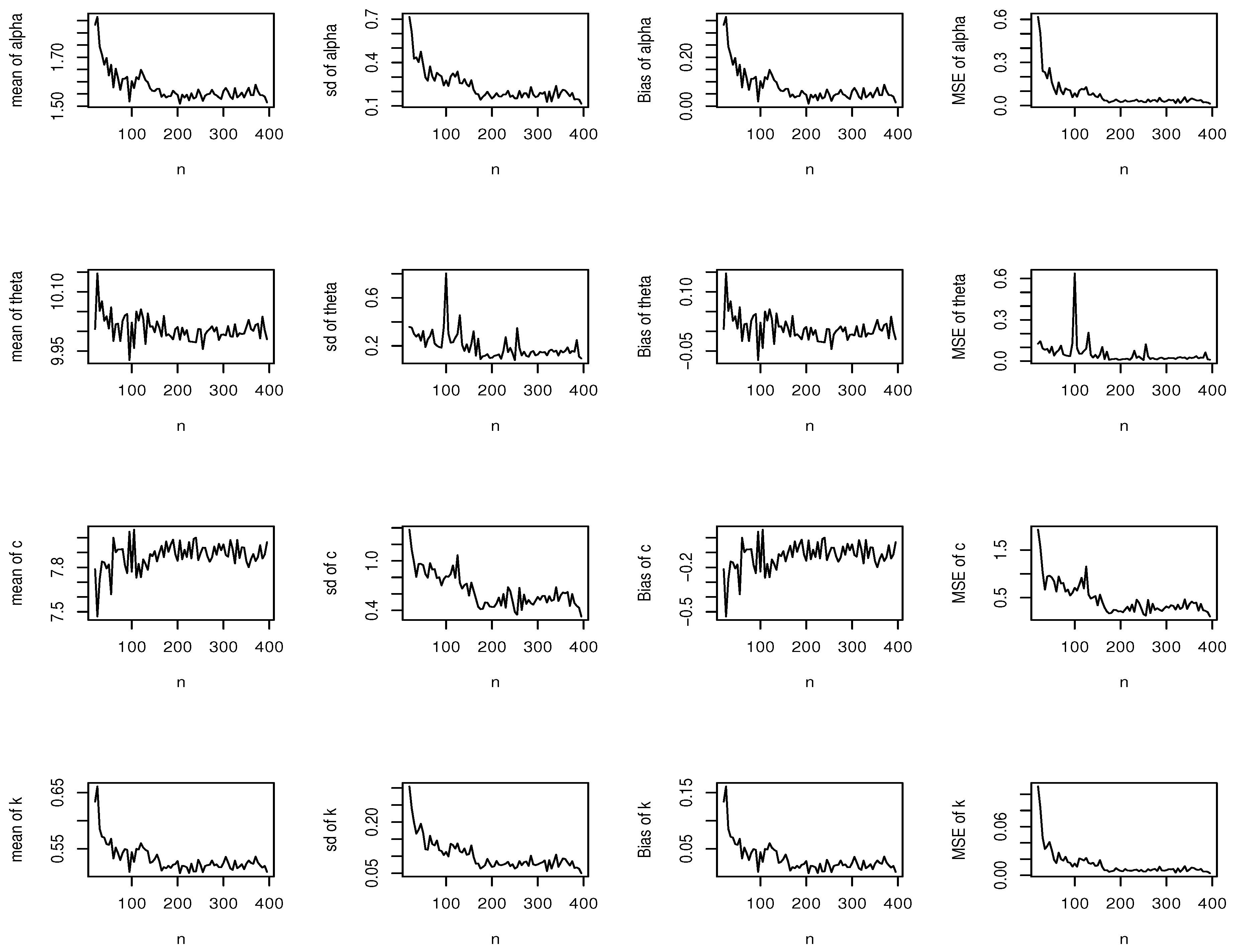
6.1. Simulation Study 1
6.2. Simulation Study 2
7. Data Analysis
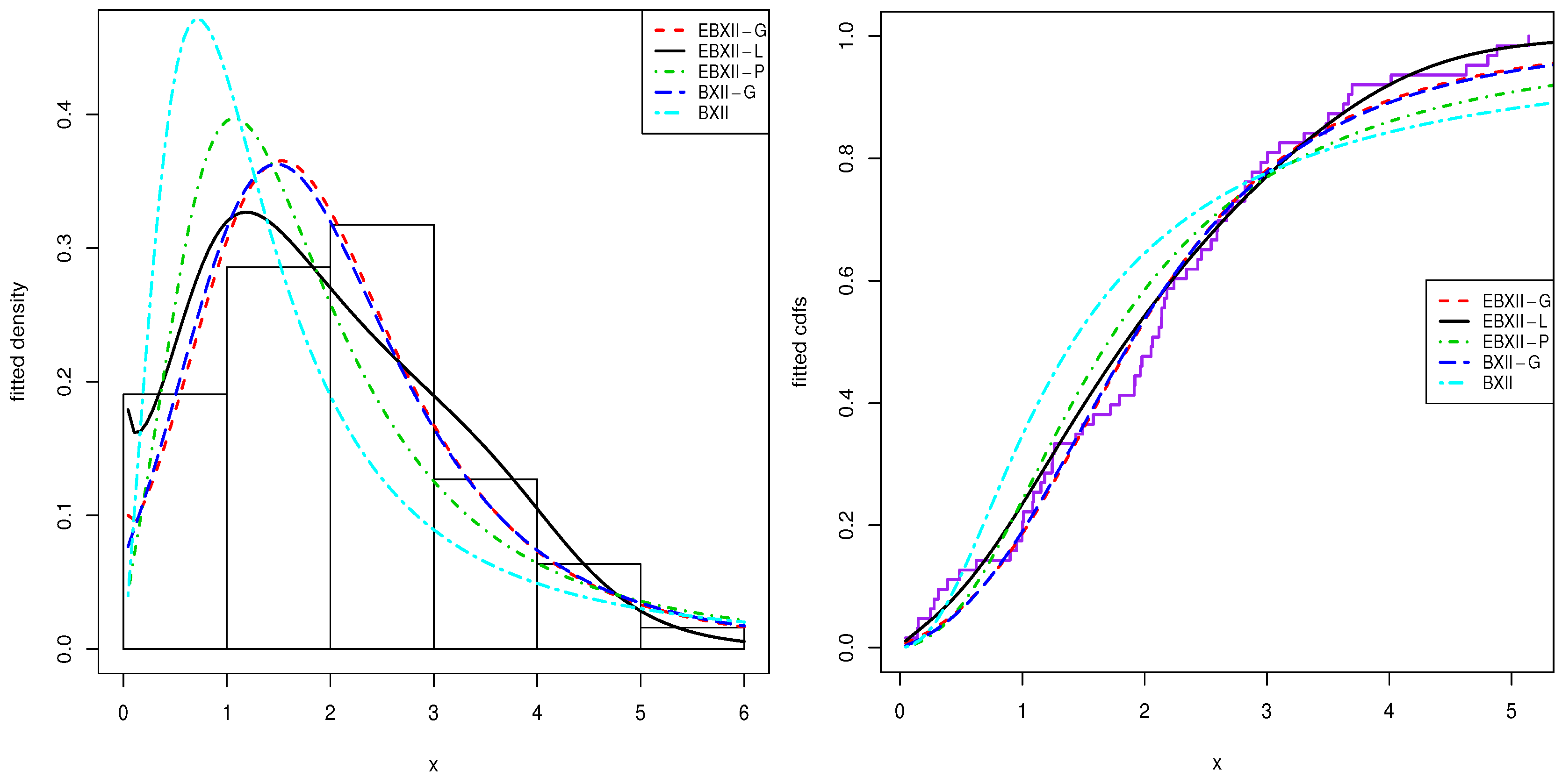
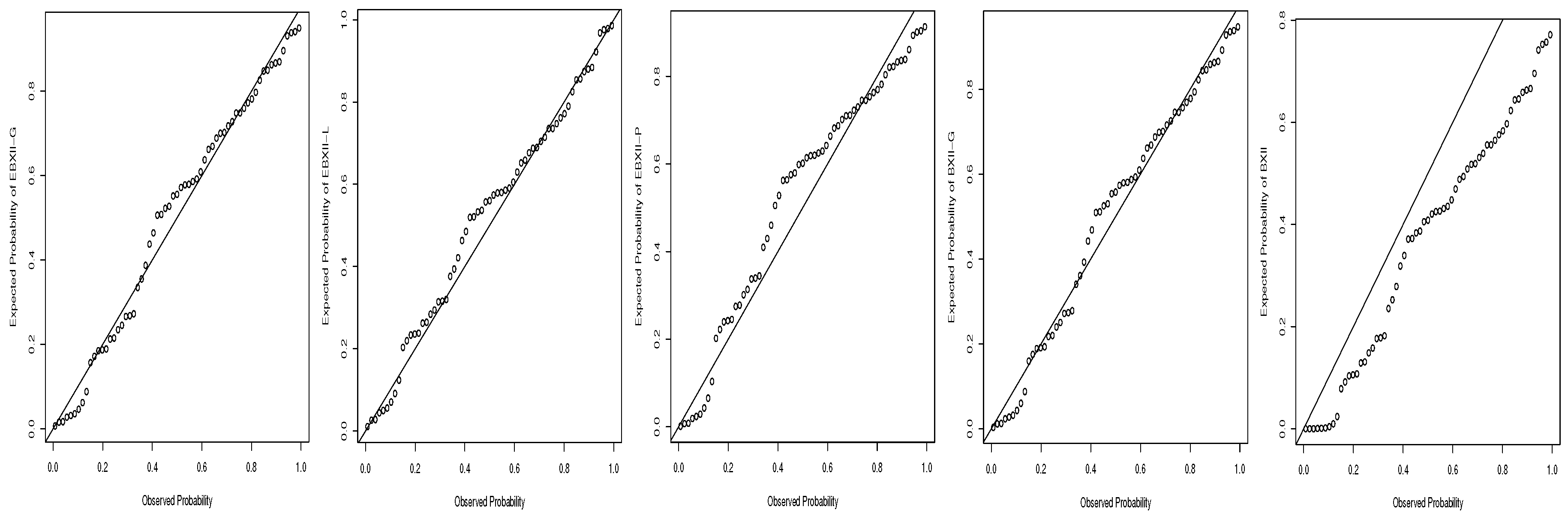
7.1. Stress Data
7.2. Service Times Data
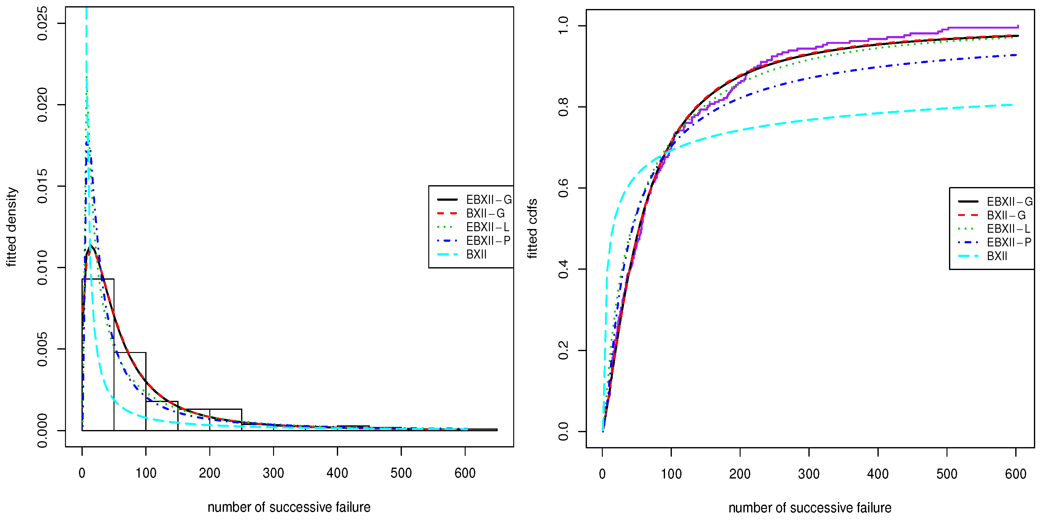
7.3. Failure Data
8. Conclusions
Author Contributions
Funding
Conflicts of Interest
References
- Paranaiba, P.F.; Ortega, E.M.; Cordeiro, G.M.; Pascoa, M.A.D. The Kumaraswamy Burr XII distribution: Theory and practice. J. Stat. Comput. Simul. 2013, 83, 2117–2143. [Google Scholar] [CrossRef]
- Al-Saiari, A.Y.; Baharith, L.A.; Mousa, S.A. Marshall-Olkin extended Burr type XII distribution. Int. J. Stat. Probab. 2014, 3, 78–84. [Google Scholar] [CrossRef]
- Gomes AE da-Silva, C.Q.; Cordeiro, G.M. Two extended Burr models: Theory and practice. Commun. Stat. Theory Methods 2015, 44, 1706–1734. [Google Scholar] [CrossRef]
- Arslan, A.M.; Tahir, M.H.; Jamal, F.; Ozel, G. A New Generalized Burr Family of Distributions for the Lifetime Data. J. Stat. Appl. Probab. 2017, 6, 401–417. [Google Scholar]
- Johnson, N.L.; Kotz, S.; Balakrishnan, N. Continuous Univariate Distributions, 2nd ed.; Jonh Wiley & Sons: New York, NY, USA, 1995; Volume 2. [Google Scholar]
- Garcia, A.; Torres, J.L.; Prieto, E.; De Francisco, A. Fitting wind speed distributions: A case study. Sol. Energy 1998, 62, 139–144. [Google Scholar] [CrossRef]
- Harris, R.I. Generalised Pareto methods for wind extremes. Useful tool or mathematical mirage. J. Wind Eng. Ind. Aerodyn. 2005, 93, 341–360. [Google Scholar] [CrossRef]
- Kantar, Y.M.; Usta, I. Analysis of Wind Speed Distribution. Energy Convers. Manag. 2008, 49, 962–973. [Google Scholar] [CrossRef]
- Carta, J.A.; Ramirez, P.; Velazquez, S. A review of wind speed probability distributions used in wind energy analysis. Renew. Sustain. Energy Rev. 2009, 13, 933–955. [Google Scholar] [CrossRef]
- Panteli, A.T.M.; Mancarella, P. Influence of extreme weather and climate change on the resilience of power systems: Impacts and possible mitigation strategies. Electr. Power Syst. Res. 2015, 127, 259–270. [Google Scholar] [CrossRef]
- Chiodo, E.; De Falco, P. The Inverse Burr Distribution for Extreme Wind Speed Prediction: Genesis, Identification and Estimation. Electr. Power Syst. Res. 2016, 141, 549–561. [Google Scholar] [CrossRef]
- Feijóo, D.V. Assessing wind speed simulation methods. Renew. Sustain. Energy Rev. 2016, 56, 473–483. [Google Scholar] [CrossRef]
- Noack, A. A Class of Random Variables with Discrete Distributions. Ann. Math. Stat. 1950, 21, 127–132. [Google Scholar] [CrossRef]
- Silva, R.B.; Cordeiro, G.M. The Burr XII power series distributions: A new compounding family. Braz. J. Probab. Stat. 2015, 29, 565–589. [Google Scholar] [CrossRef]
- Da Silva, R.V.; Gomes-Silva, F.; Ramos, M.W.A.; Cordeiro, G. The exponentiated Burr XII Poisson distribution with application to lifetime data. Int. J. Stat. Probab. 2015, 4, 112–131. [Google Scholar] [CrossRef]
- Korkmaz, M.Ç.; Erişoğlu, M. The Burr XII-Geometric Distribution. J. Selcuk Univ. Nat. Appl. Sci. 2014, 3, 75–87. [Google Scholar]
- Chen, G.; Balakrishnan, N. A general purpose approximate goodness-of-fit test. J. Qual. Technol. 1995, 27, 154–161. [Google Scholar] [CrossRef]
- Andrews, D.F.; Herzberg, A.M. Data: A Collection of Problems from Many Fields for the Student and Research Worker; Springer Series in Statistics: New York, NY, USA, 1985. [Google Scholar]
- Cooray, K.; Ananda, M.M. A generalization of the half-normal distribution with applications to lifetime data. Commun. Stat. Theory Methods 2008, 37, 1323–1337. [Google Scholar] [CrossRef]
- Murthy, D.P.; Xie, M.; Jiang, R. Weibull Models; John Wiley & Sons: Haboken, NJ, USA, 2004. [Google Scholar]
- Tahir, M.H.; Cordeiro, G.M.; Mansoor, M.; Zubair, M. The Weibull-Lomax distribution: Properties and applications. Hacet. J. Math. Stat. 2015, 44, 461–480. [Google Scholar] [CrossRef]
- Proschan, F. Theoretical explanation of observed decreasing failure rate. Technometrics 1963, 5, 375–383. [Google Scholar] [CrossRef]
- Kuş, C. A new lifetime distribution. Comput. Stat. Data Anal. 2007, 51, 4497–4509. [Google Scholar] [CrossRef]


| Distribution | Parameter Space | |||
|---|---|---|---|---|
| Poisson | ||||
| Geometric | 1 | (0,1) | ||
| Binomial | ||||
| Logarithmic | (0,1) |
| Parameters | ||||||||||||
|---|---|---|---|---|---|---|---|---|---|---|---|---|
| 2, 0.5, 0.5, 0.5 | 2.1928 | 0.5310 | 0.3114 | 2.1858 | 2.1284 | 0.5115 | 0.3696 | 2.0686 | 2.0594 | 0.5008 | 0.4321 | 2.0351 |
| (0.3739) | (0.1468) | (0.2383) | (0.5159) | (0.2951) | (0.1055) | (0.2005) | (0.4276) | (0.1405) | (0.0677) | (0.1259) | (0.2414) | |
| 1, 0.5, 3, 0.75 | 1.0621 | 0.6203 | 2.9386 | 0.6986 | 1.0569 | 0.5545 | 2.9642 | 0.7734 | 0.9722 | 0.5219 | 2.9723 | 0.7567 |
| (0.4210) | (0.2078) | (0.3679) | (0.3324) | (0.3474) | (0.1529) | (0.2411) | (0.2188) | (0.2352) | (0.0731) | (0.1793) | (0.1538) | |
| 3, 0.1, 3, 0.1 | 2.9904 | 0.1044 | 3.0617 | 0.1154 | 2.9902 | 0.1002 | 2.9978 | 0.0785 | 3.0087 | 0.1005 | 3.0027 | 0.1022 |
| (0.1310) | (0.0117) | (0.1578) | (0.1754) | (0.1053) | (0.0078) | (0.1181) | (0.1633) | (0.0805) | (0.0053) | (0.0942) | (0.1170) | |
| 5, 0.9, 2, 0.9 | 4.9810 | 0.9545 | 2.1140 | 0.8496 | 5.0138 | 0.9169 | 2.0942 | 0.8699 | 4.9976 | 0.9104 | 1.9875 | 0.8711 |
| (0.7592) | (0.1832) | (0.6073) | (0.9044) | (0.2847) | (0.0882) | (0.4431) | (0.4365) | (0.1819) | (0.0703) | (0.2970) | (0.1816) | |
| 5, 5, 5, 0.99 | 4.9483 | 4.9838 | 5.0854 | 0.9572 | 4.9415 | 5.0126 | 5.1212 | 0.9842 | 4.9743 | 4.9785 | 5.0246 | 0.9954 |
| (0.3309) | (0.2440) | (0.4827) | (0.1362) | (0.3526) | (0.2423) | (0.5678) | (0.1036) | (0.1308) | (0.1446) | (0.2212) | (0.0209) | |
| 10, 0.7, 0.5, 0.3 | 10.0795 | 0.7367 | 0.4899 | 0.2615 | 10.0686 | 0.7103 | 0.4901 | 0.2925 | 10.0355 | 0.7077 | 0.4974 | 0.3026 |
| (0.3178) | (0.2787) | (0.1950) | (0.5675) | (0.2825) | (0.2398) | (0.1558) | (0.4701) | (0.1563) | (0.2049) | (0.1341) | (0.2793) | |
| 0.8, 2, 0.2, 0.5 | 1.0035 | 1.8689 | 0.2907 | 0.4027 | 0.8862 | 1.9841 | 0.2169 | 0.5169 | 0.8488 | 1.9911 | 0.2104 | 0.5121 |
| (0.3488) | (0.4761) | (0.2087) | (0.4911) | (0.1938) | (0.3719) | (0.0883) | (0.2861) | (0.1275) | (0.2608) | (0.0616) | (0.2586) | |
| Model | |||||||||
|---|---|---|---|---|---|---|---|---|---|
| EBXII-G | 0.1837 | −2.3736 | 2.8794 | 0.7734 | 102.2356 | 212.4712 | 0.0835 | 0.8597 | 0.1276 |
| (0.0531) | (1.2987) | (0.0852) | (0.0573) | ||||||
| BXII-G | −6.5779 | 0.7905 | 3.8292 | 103.7589 | 213.5178 | 0.0907 | 1.3308 | 0.1920 | |
| (9.3669) | (0.2420) | (1.6013) | |||||||
| EBXII-L | 0.1466 | −16.6902 | 3.5208 | 0.7453 | 101.0149 | 210.0298 | 0.0761 | 0.6064 | 0.0821 |
| (0.0244) | (5.1283) | (0.0233) | (0.1067) | ||||||
| EBXII-P | 0.2237 | −1.6098 | 2.8432 | 0.6581 | 103.4967 | 214.9934 | 0.0850 | 1.2765 | 0.2155 |
| (0.0592) | (0.8678) | (0.0996) | (0.1445) | ||||||
| BurrXII | 1.1736 | 1.6327 | 108.5477 | 221.0955 | 0.1143 | 2.8873 | 0.3072 | ||
| (0.0983) | (0.1638) |
| Model | |||||||||
|---|---|---|---|---|---|---|---|---|---|
| EBXII-G | 0.3573 | −69.4175 | 1.3364 | 2.6885 | 102.0361 | 212.0721 | 0.0935 | 0.6693 | 0.0803 |
| (0.4481) | (7.6873) | (0.7013) | (1.7470) | ||||||
| BXII-G | −47.7605 | 1.0344 | 3.6365 | 102.3057 | 210.6114 | 0.0967 | 0.7748 | 0.0861 | |
| (4.0336) | (0.1569) | (0.3727) | |||||||
| EBXII-L | 0.2364 | 2.9710 | 3.0922 | 99.5671 | 207.1343 | 0.1067 | 0.4639 | 0.0860 | |
| (0.0461) | (0.4027) | (0.1331) | (0.1867) | ||||||
| EBXII-P | 1.0879 | −3.6258 | 1.4626 | 1.5307 | 108.0832 | 224.1664 | 0.1498 | 1.7402 | 0.2545 |
| (0.6565) | (1.1587) | (0.4915) | (0.6687) | ||||||
| BurrXII | 2.1335 | 0.6151 | 116.1148 | 236.2296 | 0.2545 | 10.4160 | 1.3521 | ||
| (0.2804) | (0.0982) |
| Model | |||||||||
|---|---|---|---|---|---|---|---|---|---|
| EBXII-G | 324.1786 | −59.7180 | 0.2562 | 7.4612 | 1178.5170 | 2365.0330 | 0.0410 | 0.5110 | 0.0592 |
| (0.5597) | (0.1066) | (0.0085) | (0.1257) | ||||||
| BXII-G | −349.9338 | 0.8401 | 1.7449 | 1180.261 | 2366.5210 | 0.0413 | 0.5832 | 0.0678 | |
| (1.2261) | (0.2915) | (0.5884) | |||||||
| EBXII-L | 377.6428 | −267.0753 | 0.3544 | 5.6072 | 1189.0280 | 2386.0560 | 0.1026 | 3.9962 | 0.7387 |
| (0.1188) | (0.1809) | (0.0226) | (0.2711) | ||||||
| EBXII-P | 68.2377 | −4.1156 | 0.3268 | 3.9270 | 1186.3710 | 2380.7430 | 0.0645 | 1.4650 | 0.1768 |
| (2.2356) | (0.9638) | (0.0319) | (0.3690) | ||||||
| BurrXII | 53.7460 | 0.0047 | 1335.4150 | 2674.8300 | 0.3697 | 44.8020 | 9.2016 | ||
| (1.6200) | (0.0004) |
© 2018 by the authors. Licensee MDPI, Basel, Switzerland. This article is an open access article distributed under the terms and conditions of the Creative Commons Attribution (CC BY) license (http://creativecommons.org/licenses/by/4.0/).
Share and Cite
Nasir, A.; Yousof, H.M.; Jamal, F.; Korkmaz, M.Ç. The Exponentiated Burr XII Power Series Distribution: Properties and Applications. Stats 2019, 2, 15-31. https://doi.org/10.3390/stats2010002
Nasir A, Yousof HM, Jamal F, Korkmaz MÇ. The Exponentiated Burr XII Power Series Distribution: Properties and Applications. Stats. 2019; 2(1):15-31. https://doi.org/10.3390/stats2010002
Chicago/Turabian StyleNasir, Arslan, Haitham M. Yousof, Farrukh Jamal, and Mustafa Ç. Korkmaz. 2019. "The Exponentiated Burr XII Power Series Distribution: Properties and Applications" Stats 2, no. 1: 15-31. https://doi.org/10.3390/stats2010002