Cronbach’s Alpha under Insufficient Effort Responding: An Analytic Approach

Abstract

Surveys commonly suffer from insufficient effort responding (IER). If not accounted for, IER can cause biases and lead to false conclusions. In particular, Cronbach’s alpha has been empirically observed to either deflate or inflate due to IER. This paper will elucidate how IER impacts Cronbach’s alpha in a variety of situations. Previous results concerning internal consistency under mixture models are extended to obtain a characterization of Cronbach’s alpha in terms of item validities, average variances, and average covariances. The characterization is then applied to contaminating distributions representing various types of IER. The discussion will provide commentary on previous simulation-based investigations, confirming some previous hypotheses for the common types of IER, but also revealing possibilities from newly considered responding patterns. Specifically, it is possible that the bias can change from negative to positive (and vice versa) as the proportion of contamination increases.

1. Introduction

When administering self-report surveys, there is often a class of respondents that fail to provide accurate and thoughtful responses [1]. This type of responding, referred to as careless responding or insufficient effort responding (IER) [2], can contaminate otherwise accurate data and bias statistical summaries. Intuition suggests that IER would weaken measures of the association of variables, and often it does [3]. However, recent research [4,5] has observed and discussed the non-intuitive phenomena of IER inflating measures of association.

The negative consequences of inflated measures of association due to IER are many. The effect of IER on the linear correlation coefficient has been well documented [4,6,7], and conditions causing the magnitude of correlation to inflate have been characterized. Other studies have suggested that patterned careless responses in surveys with positively and negatively keyed items can lead to misleading conclusions about the dimensionality of constructs [8,9].

Cronbach’s alpha [10] is also subject to possible inflation under IER [5,11]. Whether justified or not [12], Cronbach’s alpha is often the only reported measure of reliability. McNeish [13] found that of 118 studies published in a 21-month period in American Psychological Association flagship journals, 109 used Cronbach’s alpha as the sole assessment of reliability. Therefore the possibility of inflation due to careless responses is particularly insidious, as it is possible that researchers will overestimate an instrument’s reliability. Ultimately, this can have downstream effects on the evaluation of the study, and can make studies seem more sound than they actually are.

Work Related to Cronbach’s Alpha under IER or Mixture Models

Previous investigations into the effect of IER on Cronbach’s alpha fall into three categories: those that remove suspected IER from real data and see how the value of Cronbach’s alpha changes [2,14], those that simulate a combination of valid and careless responses and examine alpha and other statistics [5], and those that proceed by mathematical derivations. Previous works in the last category include Attali’s [15] investigation of reliability in the context of speeded multiple-choice questions, and Fong, Ho, and Lam’s [11] study which considered IER as consisting of either random or straight-lining responses, derived a formula for the bias in Cronbach’s alpha, and plotted the bias for various proportions of each kind of IER.

The present paper primarily consists of mathematical derivations with a small simulation component. The main result is a characterization of the behavior of Cronbach’s alpha under a mixture of two distributions, representing valid responses and IER. An important earlier work in this area is that of Waller [16], in which he derived an expression for the value of Cronbach’s alpha under a mixture model and illustrated through several examples how the mixture can create either a negative or positive bias. Our analysis will extend his work in two directions. First, we will relate the sign of the bias in Cronbach’s alpha to a quadratic function of the mixing proportion. The roots and leading coefficient of this function yield five mathematical possibilities. Simulation is used to show that all five possibilities are potential realities by identifying sampling scenarios that correspond to each. Second, we relate the result to IER. Six distinct observations will be made, which include not only general confirmations of previous observations from simulation studies, but also the existence of a case which we have not seen mentioned in the literature.

The intent of this paper is to demonstrate via mathematical proof all of the ways that Cronbach’s alpha can be biased, including some possibilities that are non-intuitive. As an educational aid, we include a link to a simulation app to help visualize the impact of varying proportions of IER.

The remaining sections will derive the mathematics, apply the main result in the context of IER, and conclude.

2. Mathematics for General Result

As the result builds on Waller’s [16], we adopt his notation wherever possible. Kuder and Richardson [17] defined a measure of internal reliability for binary choices (commonly known as KR-20), which was generalized by Hoyt [18] and Guttman [19] and popularized by Cronbach [10] to the form bearing his name. Let $\mathbf{V}=(V_1,V_2,\dots ,V_k)$ represent responses from a multivariate probability distribution to k items on an instrument. The notation V is used to represent the valid distribution. Cronbach’s alpha is defined as

$${\alpha }_V=\frac{k}{k-1}\left(1-\frac{{\sum }_{i=1}^k\mathrm{var}\left(V_i\right)}{\mathrm{var}\left({\sum }_{i=1}^k{V}_i\right)}\right).$$

(1)

An alternate formulation in terms of average variances and covariances will be convenient. Define $\overline{{\sigma }_{iV}^2}$ to be the average variance of components of V, and $\overline{{\sigma }_{ijV}}$ to be the average covariance between distinct components of V. Specifically,

$$\overline{{\sigma }_{iV}^2}=\frac{{\sum }_{i=1}^k\mathrm{var}\left(V_i\right)}{k}$$

and

$$\overline{{\sigma }_{ijV}}=\frac{{\sum \sum }_{i\ne j}\mathrm{cov}(V_i,V_j)}{k(k-1)}.$$

Then Cronbach’s alpha may be expressed in the form [16,20]

$$\alpha =\frac{k\overline{{\sigma }_{ijV}}}{(k-1)\overline{{\sigma }_{ijV}}+\overline{{\sigma }_{iV}^2}}.$$

(2)

Now consider an instrument with k items given to a population with two distinct subgroups. The first subgroup has a response distribution denoted by $\mathbf{V}=(V_1,V_2,\dots ,V_k)$, and the second subgroup has a response distribution denoted by $\mathbf{C}=(C_1,C_2,\dots ,C_k)$. The notation C is used to represent the contaminating IER.

Let W be a Bernoulli random variable with parameter p, where p is a value between zero and one representing the probability of observing a response from the contaminating class. That is, W is a random variable which takes value one with probability p and zero with probability $1-p$. The responses actually recorded on the instrument are described by the multivariate distribution M, defined by

$$\mathbf{M}=(1-W)\mathbf{V}+W\mathbf{C}.$$

(3)

The notation M is used to emphasize that it is a mixture of the valid and contaminating responses. Because W is either zero or one, each individual gives responses from one of the two response distributions. With probability p an individual will give contaminating responses, and with probability $1-p$ an individual will give valid responses.

By adopting this model, it is assumed that a respondent will either respond attentively to all items, or respond in an invalid manner to all items. We acknowledge that this assumption does not perfectly model real-life data; responses may be partially invalid [21] and are more likely to be invalid at the end of a survey [22]. However, we believe (and there is precedent in the literature [16]) that this assumption represents a reasonable trade-off between the realism of the assumptions and the complexity of the model. Furthermore, the usual data cleaning methods used by a practitioner to remove suspected IER operate at the respondent level rather than the item level.

The goal is to find when ${\alpha }_M>{\alpha }_V$; that is, when contamination inflates Cronbach’s alpha. First, notation and two results that will aid in the comparison are introduced.

Let ${\mu }_{iV}$ and ${\mu }_{iC}$ denote the respective means of responses to item i from the valid and contaminating distributions. The differences in these means are called “item validities” in the taxometrics literature and are denoted by ${\Delta }_i={\mu }_{iV}-{\mu }_{iC}$ [16]. As with the variances and covariances, only averages are needed. Specifically, the average product of item validities for distinct items, and the average of squared item validities:

$$\overline{{\Delta }_i{\Delta }_j}=\frac{{\sum \sum }_{i\ne j}{\Delta }_i{\Delta }_j}{k(k-1)}=\frac{{\sum \sum }_{i\ne j}({\mu }_{iV}-{\mu }_{iC})({\mu }_{jV}-{\mu }_{jC})}{k(k-1)},$$

$$\overline{{\Delta }_i^2}=\frac{{\sum }_{i=1}^k{\Delta }_i^2}{k}=\frac{{\sum }_{i=1}^k{({\mu }_{iV}-{\mu }_{iC})}^2}{k}.$$

The first of the two needed results is known as the general covariance mixture theorem [23,24]. Here, it will be expressed in terms of averages.

Lemma 1.

Let M be defined as a mixture of V and C as in Equation (3), where p is the probability of observing a response from C. Assume that the random quantities V, C, and W are independent. Then

1.

$\overline{{\sigma }_{ijM}}=(1-p)\overline{{\sigma }_{ijV}}+p\overline{{\sigma }_{ijC}}+p(1-p)\overline{{\Delta }_i{\Delta }_j}$

2.

$\overline{{\sigma }_{iM}^2}=(1-p)\overline{{\sigma }_{iV}^2}+p\overline{{\sigma }_{iC}^2}+p(1-p)\overline{{\Delta }_i^2}$

A proof is in Appendix A of Meehl [23].

The second result is an inequality between average variances and covariances of items within a distribution, and will be used to investigate special cases during the discussion.

Lemma 2.

The average of covariances between distinct components of a multivariate distribution V is less than or equal to the average variance. Symbolically,

$$\overline{{\sigma }_{ijV}}\le \overline{{\sigma }_{iV}^2}.$$

The proof is in the appendix. The main result can now be stated and proved.

Theorem 1.

Let V and C be multivariate distributions with k components representing potential responses to an instrument. Let W be a Bernoulli random variable with parameter p between zero and one. Define $\mathit{M}=(1-W)\mathit{V}+W\mathit{C}$ as a mixture of V and C. Assume that V, C, and W are independent. The behavior of Cronbach’s alpha under the mixture can be broken down into five categories.

1.

Cronbach’s alpha does not change for any mixing proportion. ${\alpha }_M={\alpha }_V$ for all p.

2.

Cronbach’s alpha inflates for any mixing proportion. ${\alpha }_M>{\alpha }_V$ for all p.

3.

Cronbach’s alpha deflates for any mixing proportion. ${\alpha }_M<{\alpha }_V$ for all p.

4.

Cronbach’s alpha inflates for small mixing proportions, but deflates for large mixing proportions. There is a value $p_0$ in the interval $(0,1)$ such that ${\alpha }_M>{\alpha }_V$ for $p<p_0$, but ${\alpha }_M<{\alpha }_V$ for $p>p_0$.

5.

Cronbach’s alpha deflates for small mixing proportions, but inflates for large mixing proportions. There is a value $p_0$ in the interval $(0,1)$ such that ${\alpha }_M<{\alpha }_V$ for $p<p_0$, but ${\alpha }_M>{\alpha }_V$ for $p>p_0$.

Furthermore, there exist distributions that will yield each of the above cases, including when the item scale is continuous, discrete, or binary.

Proof. 

The general strategy is to derive that the sign of the bias in Cronbach’s alpha has the same sign as a quadratic function of the mixing proportion p, and then invoke elementary properties of quadratic functions. Begin by finding conditions under which Cronbach’s alpha inflates, or when ${\alpha }_M-{\alpha }_V>0$. Apply Equation (2), the alternate form of Cronbach’s alpha.

$$\frac{k\overline{{\sigma }_{ijM}}}{(k-1)\overline{{\sigma }_{ijM}}+\overline{{\sigma }_{iM}^2}}-\frac{k\overline{{\sigma }_{ijV}}}{(k-1)\overline{{\sigma }_{ijV}}+\overline{{\sigma }_{iV}^2}}>0.$$

Combine into a single fraction with a common denominator.

$$k\frac{\overline{{\sigma }_{ijM}}\left((k-1)\overline{{\sigma }_{ijV}}+\overline{{\sigma }_{iV}^2}\right)-\overline{{\sigma }_{ijV}}\left((k-1)\overline{{\sigma }_{ijM}}+\overline{{\sigma }_{iM}^2}\right)}{\left((k-1)\overline{{\sigma }_{ijM}}+\overline{{\sigma }_{iM}^2}\right)\left((k-1)\overline{{\sigma }_{ijV}}+\overline{{\sigma }_{iV}^2}\right)}>0.$$

Expand the numerator. The term $(k-1)\left(\overline{{\sigma }_{ijM}}\right)\left(\overline{{\sigma }_{ijV}}\right)$ will cancel.

$$\frac{k}{\left((k-1)\overline{{\sigma }_{ijM}}+\overline{{\sigma }_{iM}^2}\right)\left((k-1)\overline{{\sigma }_{ijV}}+\overline{{\sigma }_{iV}^2}\right)}\left(\overline{{\sigma }_{iV}^2}\overline{{\sigma }_{ijM}}-\overline{{\sigma }_{ijV}}\overline{{\sigma }_{iM}^2}\right)>0.$$

(4)

The denominator of (4) is a scaled product of variances and must be positive, so it will not affect the sign of the bias. Thus, to determine whether Cronbach’s alpha has inflated, it suffices to find when

$$\overline{{\sigma }_{iV}^2}\overline{{\sigma }_{ijM}}-\overline{{\sigma }_{ijV}}\overline{{\sigma }_{iM}^2}>0.$$

Apply the general covariance mixture theorem to the average variances and covariances of M.

$$\overline{{\sigma }_{iV}^2}\left((1-p)\overline{{\sigma }_{ijV}}+p\overline{{\sigma }_{ijC}}+p(1-p)\overline{{\Delta }_i{\Delta }_j}\right)-\overline{{\sigma }_{ijV}}\left((1-p)\overline{{\sigma }_{iV}^2}+p\overline{{\sigma }_{iC}^2}+p(1-p)\overline{{\Delta }_i^2}\right)>0.$$

Expand and group terms that include $p^2$ and p. The term $(1-p)\overline{{\sigma }_{iV}^2}\overline{{\sigma }_{ijV}}$ will cancel. The result is

$$\left(\overline{{\sigma }_{ijV}}\overline{{\Delta }_i^2}-\overline{{\sigma }_{iV}^2}\overline{{\Delta }_i{\Delta }_j}\right)p^2+\left(\overline{{\sigma }_{iV}^2}\overline{{\sigma }_{ijC}}-\overline{{\sigma }_{ijV}}\overline{{\sigma }_{iC}^2}-\overline{{\sigma }_{ijV}}\overline{{\Delta }_i^2}+\overline{{\sigma }_{iV}^2}\overline{{\Delta }_i{\Delta }_j}\right)p>0.$$

Define a and b as

$$\begin{array}{cc}\hfill a& =\overline{{\sigma }_{ijV}}\overline{{\Delta }_i^2}-\overline{{\sigma }_{iV}^2}\overline{{\Delta }_i{\Delta }_j},\hfill \end{array}$$

(5)

$$\begin{array}{cc}\hfill b& =\overline{{\sigma }_{iV}^2}\overline{{\sigma }_{ijC}}-\overline{{\sigma }_{ijV}}\overline{{\sigma }_{iC}^2}-\overline{{\sigma }_{ijV}}\overline{{\Delta }_i^2}+\overline{{\sigma }_{iV}^2}\overline{{\Delta }_i{\Delta }_j}=\overline{{\sigma }_{iV}^2}\overline{{\sigma }_{ijC}}-\overline{{\sigma }_{ijV}}\overline{{\sigma }_{iC}^2}-a.\hfill \end{array}$$

(6)

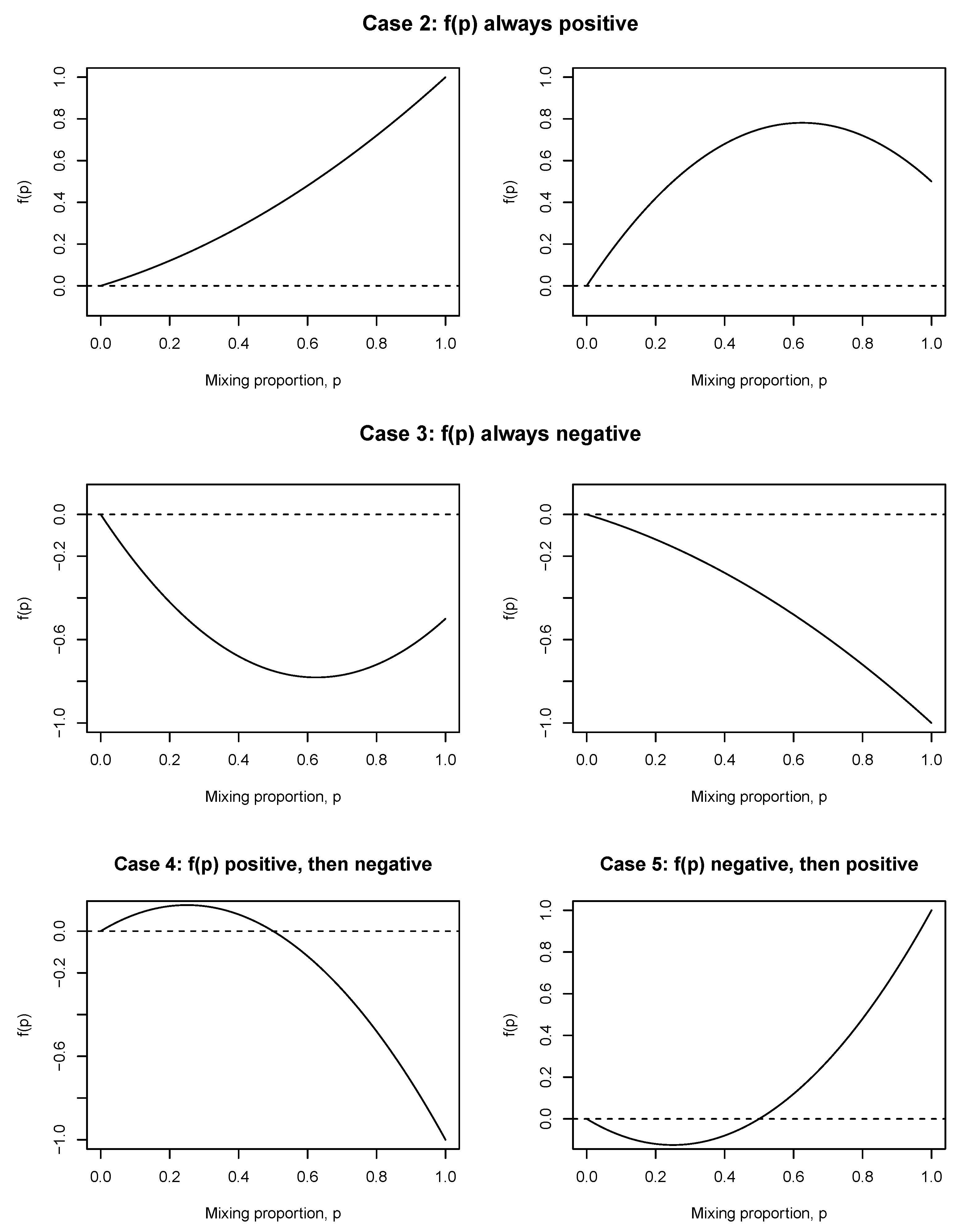
It is now easy to see that Cronbach’s alpha inflates when $f\left(p\right)=a{p}^2+bp>0$. $f\left(p\right)$ is a quadratic with no constant term. This is a simple family of functions, though the coefficients are not simple. Momentarily ignore how a and b are defined (we will return to this soon), and consider the possible behaviors of functions of the form $f\left(p\right)=a{p}^2+bp$. In particular, we are interested in the sign for values of p in the interval $(0,1)$, as this will determine when Cronbach’s alpha inflates or deflates. This behavior can be characterized in terms of the concavity and roots of $f\left(p\right)$. The roots are at 0 and $-b/a$ (as long as $a\ne 0)$. Consider each case in turn.

• Case one is a trivial possibility when $a=b=0$. $f\left(p\right)=0$ for all p in $(0,1)$.
• Case two is $f\left(p\right)>0$ for all p in $(0,1)$. This has two subcases: if $a\ge 0$ and $b\ge 0$ (but not both $a=b=0$), or if $0<-a\le b$.
• Case three is $f\left(p\right)<0$ for all p in $(0,1)$. This has two subcases: if $a\le 0$ and $b\le 0$ (but not both $a=b=0$), or if $b\le -a<0$.
• Case four occurs when $0<b<-a$. The non-zero root $p_0$ lies in the interval $(0,1)$, meaning $f\left(p\right)$ changes sign at $p_0$. Because $a<0$ the function is concave down, so the bias changes from positive to negative.
• Case five occurs when $-a\le b<0$. The non-zero root $p_0$ is in the interval $(0,1)$, except now $a>0$ and the function is concave up. The bias changes from negative to positive.

Examples of each non-trivial case, including the subcases for two and four, are included in Figure 1.

Because the sign of the bias is derived to be the same as the sign of a quadratic function with a root at zero, these scenarios are exhaustive. For example, a scenario in which Cronbach’s first deflates, then inflates, and deflates again as p increases would require three crossings of the horizontal axis. This is not possible for a quadratic and is logically excluded.

To complete the proof, remember that the values a and b are not arbitrary, but defined in Equations (5) and (6) in terms of summaries of two multivariate probability distributions which represent responses to an instrument. Item validities, representing differences in means, are bounded by the item scale. Variances and covariances are also limited by the range of the scale and inequalities such as Cauchy-Schwarz [25]. Furthermore, if the scale has a small number of discrete options or is binary, then means, variances, and covariances are not independent parameters. A natural question is: are all five cases actually possible? The answer is yes, and the following two paragraphs describe how to obtain each.

Consider an instrument with 20 items on a five-point scale from one to five. No questions use negative keying. Discrete data are produced by first generating multivariate normal observations with a given mean vector and covariance matrix, and then rounding. The covariance matrix is constructed by using the average variance for the diagonal entries and the average covariance for the off-diagonal entries. The multivariate normal observations are rounded to the nearest integer in the scale. Forcing discrete responses by rounding will, of course, change the means, variances, and covariances, but in the particular cases considered, the change is not enough to alter the characterization of Cronbach’s alpha. Two data sets are produced, representing valid responses and mixed responses. Cronbach’s alpha is calculated for each, and the bias is recovered as the difference. This simulation is repeated for values of p, the mixing proportion, in increments of 0.025 between zero and one.

Table 1. Summaries of V and C (before discretization) for producing each case in the context of a scale with five options.

	Means of V	$\overline{{\mathit{\sigma }}_{\mathit{iV}}^2}$	$\overline{{\mathit{\sigma }}_{\mathit{ijV}}}$	Means of C	$\overline{{\mathit{\sigma }}_{\mathit{iC}}^2}$	$\overline{{\mathit{\sigma }}_{\mathit{ijC}}}$
Case 1	${\mu }_{iV}=3$ for all items	2	1	${\mu }_{iC}=3$ for all items	2	1
Case 2	${\mu }_{iV}=2$ for all items	1	0	${\mu }_{iC}=4$ for all items	1	0
Case 3	${\mu }_{iV}=2$ for all items	2	1.5	${\mu }_{iC}=4$ for all items	6	0
Case 4	${\mu }_{iV}=2$ for all items	1	0.5	${\mu }_{iC}=4$ for all items	1	0
Case 5	${\mu }_{iV}=3$ for all items	1	0.2	${\mu }_{iV}=1$ for odd items;	1	0.8
				${\mu }_{iV}=5$ for even items

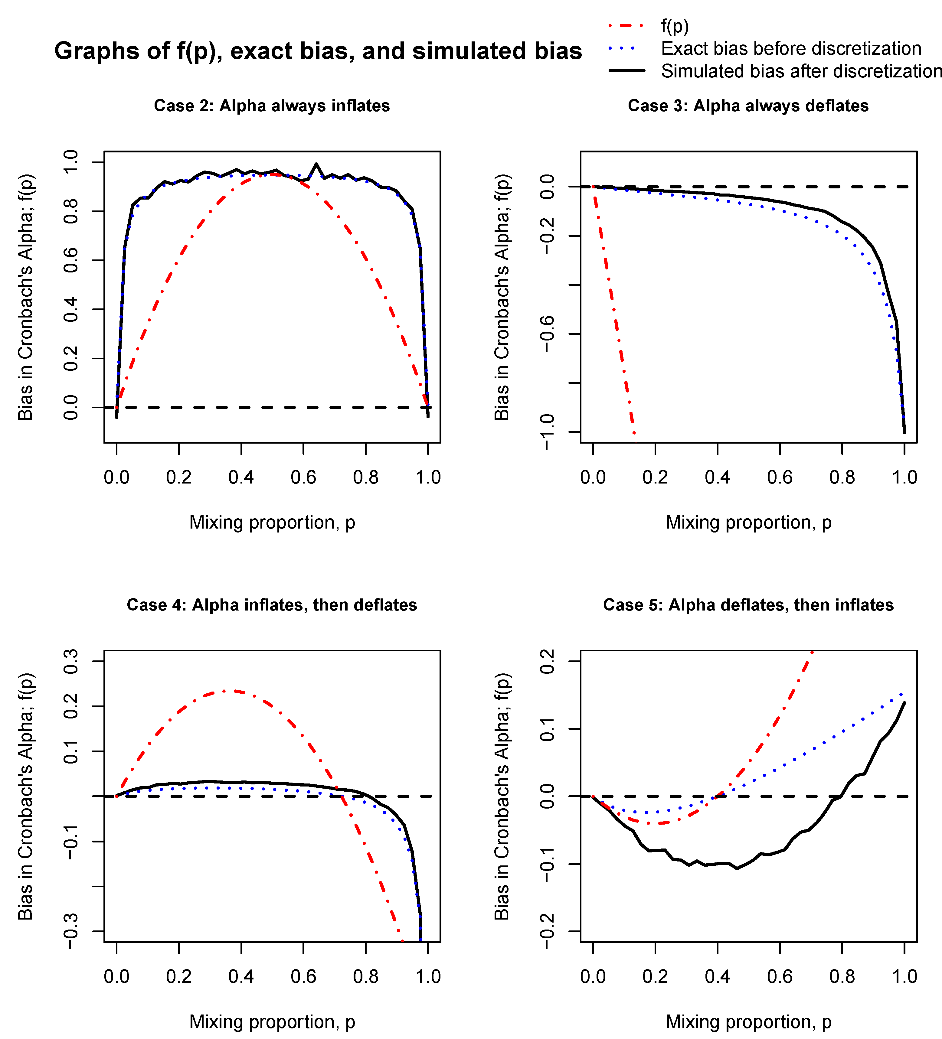
describes the means, variances, and covariances of the multivariate normal values which were rounded to obtain V and C in order to reproduce each case. Figure 2 shows, for each case, the bias of the simulation as a solid black line, the exact bias before discretization as a dotted blue line, and the function $f\left(p\right)$ as a dot-dash red line. To aid in seeing when the sign changes, there is a dashed line for the horizontal axis. The simulations used 10,000 respondents at each value of p.

Reproducing all cases when all items are binary options is trickier, but still possible. The data were simulated in the same manner as before, except responses were rounded to the nearest of zero or one.

Table 2. Summaries of V and C (before discretization) for producing each case in the context of a scale with binary options.

	Means of V	$\overline{{\mathit{\sigma }}_{\mathit{iV}}^2}$	$\overline{{\mathit{\sigma }}_{\mathit{ijV}}}$	Means of C	$\overline{{\mathit{\sigma }}_{\mathit{iC}}^2}$	$\overline{{\mathit{\sigma }}_{\mathit{ijC}}}$
Case 1	${\mu }_{iV}=0.5$ for all items	1	0.5	${\mu }_{iC}=0.5$ for all items	1	0.5
Case 2	${\mu }_{iV}=0.4$ for all items	1	0	${\mu }_{iC}=0.6$ for all items	1	0.8
Case 3	${\mu }_{iV}=0.4$ for all items	0.5	0.4	${\mu }_{iC}=0.6$ for all items	1	0
Case 4	${\mu }_{iV}=0.2$ for all items	0.3	0.1	${\mu }_{iC}=0.8$ for all items	0.3	0
Case 5	${\mu }_{iV}=0.5$ for all items	1	0.3	${\mu }_{iC}=0$ for odd items;	0.5	0.2
				${\mu }_{iC}=1$ for even items

describes the summaries of the multivariate normal values which were rounded to obtain V and C in order to reproduce each case. A larger number of simulations was necessary to reduce the sampling variability and clearly see the bias in Cronbach’s alpha. We found 20,000 to be sufficient for all except case five, which used 100,000 simulations. The graphs for the binary case are not significantly different from the five-option case, and are omitted. This completes the proof. □

We illustrate one of the non-intuitive possibilities, case 2, through an example with simulated data.

Table 3. An example of data simulated from case 2. Each class is inconsistent, with estimates of Cronbach’s alpha being 0.13 for the valid class and 0.063 for the contaminating class, yet the combined data set estimates alpha as 0.87.

Respondent	Response Class	Q1	Q2	Q3	Q4	Q5
1	Contaminating	4	5	4	3	4
2	Valid	3	1	3	1	1
3	Valid	1	1	1	1	2
4	Valid	1	2	4	2	1
5	Contaminating	4	4	3	2	4
6	Valid	1	1	1	1	2
7	Valid	2	3	1	2	2
8	Contaminating	3	5	3	5	5
9	Contaminating	3	5	3	4	3
10	Valid	2	2	4	2	1

contains data from ten respondents for an instrument with five items. The data were generated such that there was a $p=0.5$ chance of a contaminating response. In this sample, the result was six valid responses and four contaminating responses. Each class has a variance of one for all items and a covariance of zero (due to independence) between any pair of items. Because any pair of items has independent responses, the exact value for Cronbach’s alpha is zero, which is estimated from this sample to be 0.13 for the valid class and 0.063 for the contaminating class. However, because the valid class has a mean of two and the contaminating class has a mean of four, responses appear to be consistent when the two classes are combined into a single data set. The resulting estimate of Cronbach’s alpha for the entire sample is 0.87, a value generally seen as desirable, yet we see it is only due to contamination in the sample.

Now let us relate this example to Theorem 1. The contaminating classes have summaries ${\mu }_{iV}=2$, ${\mu }_{iC}=4$, $\overline{{\sigma }_{iV}^2}=1$, $\overline{{\sigma }_{iC}^2}=1$, $\overline{{\sigma }_{ijV}}=0$, and $\overline{{\sigma }_{ijC}}=0$. Applying Equations (5) and (6), we see:

$$\begin{array}{cc}\hfill a& =\overline{{\sigma }_{ijV}}\overline{{\Delta }_i^2}-\overline{{\sigma }_{iV}^2}\overline{{\Delta }_i{\Delta }_j}=0·4-1·4=-4,\hfill \\ \hfill b& =\overline{{\sigma }_{iV}^2}\overline{{\sigma }_{ijC}}-\overline{{\sigma }_{ijV}}\overline{{\sigma }_{iC}^2}-a=1·0-0·1-(-4)=4.\hfill \end{array}$$

As $0<-a=b$, this is case 2 of Theorem 1, so Cronbach’s alpha will inflate for any proportion p of contamination.

For this example, we estimated Cronbach’s alpha using Equation (1) with sample estimates of variance, but most software solutions have built-in functions with helpful features. For example, the alpha() function in the psych package [26] in R [27] produces a confidence interval for alpha and an analysis of how alpha will change if items are removed from this instrument.

At this point, no claim is made as to how likely each case is, only that all are possible. In the discussion, we will demonstrate that each of these cases could potentially be arrived at through specific types of IER.

Because of the removal of the positive term in Equation (4), $f\left(p\right)$ does not give the magnitude of the bias, but is a function with the same sign as the bias. The cancelled term includes covariances of M which implicitly depend on p, so the magnitude of the bias is a ratio of polynomials in p and is more difficult to analyze. Figure 2 makes it clear that $f\left(p\right)$ and the magnitude of the exact bias share the same roots and sign but potentially very different magnitudes. This is why the cases in Table 1 and Table 2 and Figure 2 do not differentiate between $f\left(p\right)$ being concave or convex; that property is not necessarily shared with the magnitude of the bias.

The simulation code that produced Figure 2 is available through a Shiny R [28] web app found at https://alphaier.shinyapps.io/cronbachs_alpha_under_ier/. The app allows users to investigate how Cronbach’s alpha will behave under a mixture model consisting of discretized multivariate normal distributions with any mean vector, average variance, and average covariance (as long as the resulting covariance matrix is valid). We see two potential uses for this tool. The first is educational, as it allows the user to visualize the effects of contamination on Cronbach’s alpha and test the effect when the valid and contaminating distributions are altered. Second, the forthcoming discussion relates Theorem 1 to the two main types of IER, but IER could potentially manifest through myriad possible response distributions. For any other hypothesized pattern of IER, if the means, variances, and covariances can be specified, this tool can immediately determine the effect of that contamination on Cronbach’s alpha.

The reader is reminded that the preceding is true for any mixture of two distributions, whether the interpretation of “valid” and “contaminating” holds or not.

3. Discussion and Special Cases

This section refers repeatedly to the quadratic coefficients a and b, which were defined as

$$\begin{array}{cc}\hfill a& =\overline{{\sigma }_{ijV}}\overline{{\Delta }_i^2}-\overline{{\sigma }_{iV}^2}\overline{{\Delta }_i{\Delta }_j},\hfill \\ \hfill b& =\overline{{\sigma }_{iV}^2}\overline{{\sigma }_{ijC}}-\overline{{\sigma }_{ijV}}\overline{{\sigma }_{iC}^2}-\overline{{\sigma }_{ijV}}\overline{{\Delta }_i^2}+\overline{{\sigma }_{iV}^2}\overline{{\Delta }_i{\Delta }_j}=\overline{{\sigma }_{iV}^2}\overline{{\sigma }_{ijC}}-\overline{{\sigma }_{ijV}}\overline{{\sigma }_{iC}^2}-a.\hfill \end{array}$$

With effort, these complicated coefficients yield much information about the behavior of Cronbach’s alpha under mixture models.

Now we relate the behavior of Cronbach’s alpha to IER. Studying IER in any generality is difficult because IER can take so many forms. IER is defined more by what the responses are not, rather than by what they are. For this reason, past investigations [5,11] have typically considered two extreme forms through which IER may manifest:

• Random responding: Item responses are uniformly and independently chosen from those available.
• Straight-lining: The respondent chooses the same option for all items, either in an attempt to complete the instrument as quickly as possible or operating on the belief that all questions are sufficiently similar to the first. Different respondents may choose different options, but each respondent repeats their choice without deviation.

A strength of the current approach is that any form of IER can be investigated as long as the means, average variance, and average covariance can be determined. Some of the following observations will refer specifically to random responding or straight-lining, and the fifth observation will deal with a potential form of IER we have not seen studied in the literature.

Observation 1: If all components of V have a common mean, and all components of C have a common mean, then the quadratic coefficient a cannot be positive. Cases one through four are still possible, but case five is not.

Suppose that all means are equal within a response distribution, that is, ${\mu }_{iV}={\mu }_{jV}$ and ${\mu }_{iC}={\mu }_{jC}$ for all items i and j. This implies $\overline{{\Delta }_i^2}=\overline{{\Delta }_i{\Delta }_j}$, and so Equation (5) can be simplified as

$$a=\left(\overline{{\sigma }_{ijV}}-\overline{{\sigma }_{iV}^2}\right)\overline{{\Delta }_i^2}.$$

(7)

$\overline{{\Delta }_i^2}$ is an average of squares and is clearly positive, while Lemma 2 implies the term in parentheses is negative. Thus, a is non-positive, precluding the possibility of case five.

Actually, the assumption of common means within a distribution is stronger than necessary, as it is sufficient for all item validities to be equal. However, the case of common means within a distribution is an important special case for many of the following observations, so that is the form in which the observation is stated.

Observation 2: The forces pressuring Cronbach’s alpha to inflate are:

• Increasing the differences between means of V and C when item validities have the same sign,
• Increasing the ratio of average covariance to variance for the contaminating distribution,
• Decreasing the ratio of average covariance to variance for the valid distribution.

Likewise, forces in the opposite direction will pressure Cronbach’s alpha to deflate.

The first part of this observation is easiest to see when response distributions have common means, so consider $a\ne 0$ as expressed in Equation (7). As the difference in means grows, a becomes more negative and b becomes more positive. This moves in the direction of cases two and four, so alpha tends to inflate. This is pertinent to situations in which the content of the survey will lead the mean of attentive responses to be close to an extreme bound. Consider a survey attempting to detect a rare trait like psychopathy. The mean of attentive responses is expected to be low, but if careless responses are chosen randomly and have a mean close to the midpoint of the scale, it is possible that alpha will inflate due to IER. This suggests that measures of extreme psychopathology may report inflated values of Cronbach’s alpha.

The second part of this observation is intuitively plausible, as it corresponds to contaminating with a highly internally consistent distribution, such as straight-lining. As the average covariance of C increases, b becomes more positive, moving away from case three towards case two, possibly moving through cases four and five.

The third part of this observation corresponds to a valid distribution with low internal consistency, leaving ample opportunity for inflation. As the average covariance of V decreases, a becomes more negative, which by itself would pressure alpha towards deflation, but b includes $-a$ in the sum, so b is becoming more positive. Also, the second term in b includes a negative average covariance of V. Thus, b is increasing faster than a is decreasing, moving in the direction of case two and possibly case four.

Observation 3: If means are equal across items and distributions and contamination consists purely of random responses, then Cronbach’s alpha must deflate (except for the unusual case that ${\alpha }_V\le 0$). However, if the distributions have different means, either inflation or deflation is possible.

The key characteristic of random responding is the independence between responses, so $\overline{{\sigma }_{ijC}}=0$. All means being equal implies that all item validities are zero, thus $a=0$. Combining these observations, $b=-\overline{{\sigma }_{ijV}}\overline{{\sigma }_{iC}^2}$. The assumption that ${\alpha }_V>0$ implies $\overline{{\sigma }_{ijV}}>0$, so b is negative. This is case three, in which Cronbach’s alpha deflates. The example of case three in Table 1 illustrates this exact situation.

However, if the means of V and C are not equal, then deflation is not guaranteed. Consider case two in Table 1 and Figure 2, in which the contaminating distribution has independent responses, yet alpha always inflates due to the difference in means. Case four also uses a contaminating distribution with independent observations, but whether alpha inflates or deflates depends on the exact mixing proportion p. Case two is noteworthy because both of the distributions contributing to the mixture have average covariances of zero (thus ${\alpha }_V={\alpha }_C=0$), yet the mixture has a positive value of Cronbach’s alpha. This scenario is discussed by Waller [16] as admittedly contrived and non-realistic, but useful as an example of the non-intuitive nature of reliability measures under mixtures.

The scenario of contamination with random responses is included in the simulation study of DeSimone et al. [5]. Prior to the study, the authors state the expectation that random responding will reduce alpha (p. 312). Figure 2 of the same article confirms that for their particular situation, random responses did indeed result in a strict decrease in Cronbach’s alpha. However, the results of the present article show that this is not the only possibility, and that random responses can increase Cronbach’s alpha if the means of the valid and contaminating distributions are sufficiently different.

Observation 4: Assume the valid distribution has a common mean and no questions use reverse keying. If contamination consists purely of straight-lining, then alpha is guaranteed to inflate.

The key characteristic of straight-lining respondents is that covariance equals the variance, which can be seen from applying $C_i=C_j$ to the definition of covariance. Furthermore, straight-lining forces a common mean. Thus, the item validities are all identical, and from Observation 1 a is negative. Combining with the fact $\overline{{\sigma }_{ijC}}=\overline{{\sigma }_{iC}^2}$ and Lemma 2, b can be simplified as

$$b=\overline{{\sigma }_{iC}^2}\left(\overline{{\sigma }_{iV}^2}-\overline{{\sigma }_{ijV}}\right)-a\ge -a>0.$$

This is case two, so Cronbach’s alpha can only inflate. This confirms generally the expectation by DeSimone et al. [5] that pure straight-lining will inflate alpha.

Observation 5: If contamination is of a form that alternates between extremes, then case five is a possibility. Cronbach’s alpha deflates for small p, but inflates for larger p.

Consider a mischievous responder who deliberately alternates between the first and last option in a scale for the entirety of the instrument. This form of IER can produce case five. We are not aware of (nor would we expect) any studies of this contrived style of response (though anecdotally, one of the authors observed a classmate exhibit this behavior on a standardized test in secondary school). This is case five in Table 1 and Figure 2. This could also be produced by straight-lining respondents when the survey alternates between regular and reverse keying.

Observation 6: To investigate the effects of multiple types of IER occurring simultaneously, mixture models and the general covariance mixture theorem can be applied iteratively.

In reality, IER rarely consists exclusively of purely random or straight-lining responses. It is more likely that non-valid responses from C are themselves a mixture of random, straight-lining, and perhaps other kinds of IER. Therefore the general covariance mixture theorem (Lemma 1 in the present paper) can be applied repeatedly to obtain the parameters of C, at which point Theorem 1 can be applied to determine whether Cronbach’s alpha will deflate or inflate.

Consider the following illustrative example. An instrument has five questions, with each having five options. Of the respondents, 75% will answer in a valid manner, 20% will answer randomly, and 5% will straight-line. The valid responses follow a discrete uniform with ${\alpha }_V=0.4$, corresponding to a common mean ${\mu }_{iV}=3$, an average variance of $\overline{{\sigma }_{iV}^2}=2$ and an average covariance of $\overline{{\sigma }_{ijV}}=0.235$. Careless responses come in two forms. The 20% of respondents who respond randomly (denote corresponding quantities with the subscript R) have a common mean ${\mu }_{iR}=3$, an average variance of $\overline{{\sigma }_{iR}^2}=2$, and an average covariance of $\overline{{\sigma }_{ijR}}=0$. The 5% of respondents who straight-line (denote corresponding quantities with the subscript S) choose the first item uniformly, so these responses have a common mean ${\mu }_S=3$, an average variance of $\overline{{\sigma }_{iS}^2}=2$, and an average covariance of $\overline{{\sigma }_{ijS}}=2$. All means are identical, so item validities are zero. Within the contaminating class, 80% come from random responses and 20% are straight-line responses, so an application of Lemma 1 yields $\overline{{\sigma }_{iC}^2}=0.8\times 2+0.2\times 2=2$, and $\overline{{\sigma }_{ijC}}=0.8\times 0+0.2\times 2=0.04$. Next, applying Equations (5) and (6) yields $a=0$ and $b=2\times 0.04-0.235\times 2=-0.39<0$, so this is case three, where Cronbach’s alpha will always deflate. It is interesting that for this example, only the mixing proportion within the contaminating class is important. The more numerous random responders have a larger effect than the few straight-lining responders, so changing the mixture proportion between the valid and contaminating class may change the magnitude of the bias, but will not alter the fact that Cronbach’s alpha will deflate due to contamination.

In the previous example, the random responding followed a uniform distribution (a sort of pure randomness). There are infinite other potential response distributions, but fortunately, a full specification of the exact distribution is not necessary. The behavior of Cronbach’s alpha depends on the valid and contaminating distributions only through the variances, covariances, and differences in means. So, in a partial sense, the realm of possibilities is reduced. Any multivariate distribution of responses with identical means, variances, and covariances will bias Cronbach’s alpha in the same manner.

How do real-life manifestations of careless responses tend to affect Cronbach’s alpha? For an answer, we defer to studies with real data where alpha is calculated with and without suspected IER. Huang et al. [2] compared alpha for 30 facets and found that generally alpha decreases as a result of careless responses, with a notable exception: one section with eight positively keyed and only two negatively keyed items manifested in an increase in alpha, which the authors attribute to straight-lining respondents, which is consistent with the present analysis. Wertheimer [14] conducted a similar analysis for multiple data sets and classified respondents as conscientious, random, or patterned. In summary, removing random respondents tended to increase alpha, removing patterned respondents tended to decrease alpha, and removing both tended to increase alpha, but to a lesser degree. This agrees with the results of the present paper, lending evidence that the mathematical assumptions are not too unrealistic.

4. Conclusions

This paper has presented a mathematical analysis of the behavior of Cronbach’s alpha when responses are contaminated with a secondary distribution, with a discussion emphasizing the implications for contamination from careless responses.

One limitation is the assumption that a respondent will answer all questions in either a valid or non-valid manner. In reality, some individuals will become weary part-way through a survey and begin to answer carelessly, or give careless answers to items that demand a greater deal of thought. On one hand, this simplification makes a mathematical analysis feasible, reveals the possibility of behavior not mentioned in previous IER literature (case 5), and offers mathematical certainty whenever the assumption is met. On the other hand, because the model excludes the possibility of partial IER by an individual, the conclusions reached in this investigation will not apply perfectly to real-life manifestations of IER. This is a weakness likely to affect any conceptual research into IER, as any model general enough to encompass all possible IER patterns is probably too broad to reach any specific conclusions. More complex models may allow the relaxation of this assumption, such as specifying probabilities of careless responses based on cognitive load and distance into the instrument, or modeling the number of items a respondent will answer validly before answering carelessly from that point on. Such models may not allow for a tractable analysis, and might be better suited for simulation studies. Another possibility is applying person-fit statistics [29,30] and item-response theory [31] to investigations of reliability under IER.

This paper does not address the issue of how a researcher should deal with IER. The reader is referred to one of the many articles detailing methods for detecting and removing IER [2,32,33,34,35].

Though not the only measure of reliability, Cronbach’s alpha is the most common. This paper should not be viewed as an indictment of a deficiency unique to Cronbach’s alpha, but alpha is the first natural choice for investigating the effect of IER on internal consistency. Investigation into the effect of IER on other measures of reliability, including beta [36] or ${\omega }_h$ [37], is a possible avenue for future research.

Hopefully, the analysis in this paper will increase understanding of how Cronbach’s alpha will behave under IER, and convince practitioners that IER is a threat to high quality research. In particular, except for the special cases of straight-lining when no questions use reverse keying and random responding with the same mean, IER can cause Cronbach’s alpha to behave in non-intuitive and unpredictable ways. Because Cronbach’s alpha can inflate due to IER, practitioners should be aware that a high value of alpha does not imply respondents were sufficiently attentive; it may be due to straight-lining or random responding with a different mean. In the other direction, random responding with a mean similar to the valid responses can decrease Cronbach’s alpha, underestimating the reliability of an instrument. We suggest a best practice is that measures for prevention, detection and removal of IER take place before analysis [32], especially calculations of reliability.