1. Introduction
The topic of this article is a saddlepoint approximation to the distribution of the M-statistic
, precisely
, which is the implicit solution with respect to (w.r.t.)
t of
where the function
:
is continuous (thus measurable), decreasing in its second argument, for
,
, and where the random variables
are nonnegative, dependent and satisfy
, for some fixed
. Decreasing is meant in the strict sense. The sample vector
takes values in a simplex. It is often referred to as compositional data, by referring to the situation where
represents the number of units of the
jth category, for
, given
n possible categories (see e.g., [
1]). When
follows the multinomial distribution, it is also referred to as categorical data. We consider three discrete and one continuous joint distributions for
and relate these multivariate distributions to three general urn sampling schemes that are given, e.g., in [
2].
The derivation of the saddlepoint approximation to the distribution of
relies on the distributional equivalence
which means that
has the conditional distribution of
given
. The nonnegative random variables
form a conditional triangular array in the sense that, conditionally on their sum, they are independent and their individual distributions may depend on
n. We refer to Equation (
2) as the conditional representation of
in terms of
. The computation of the distribution of
, as function of the dependent random variables
, is generally difficult. It is however simplified by replacing these dependent random variables by the triangular array random variables
, in the same order, conditional on their sum. Gatto and Jammalamadaka [
3] extended the saddlepoint approximation for tail probabilities of Skovgaard [
4] to M-statistics and used the conditional representation in Equation (
2) to derive saddlepoint approximations for important classes of nonparametric tests, such as tests based on spacings, two-sample tests based on spacing-frequencies and various tests based on ranks. The application of this conditional saddlepoint approximation to the computation of quantiles can be found in [
5]. Further applications can be found in [
6,
7].
This article presents the conditional saddlepoint approximation from the general perspective of the urn sampling model. Four cases of the of conditional representations given in Equation (
2) are related to the urn model: the joint multinomial in terms of Poisson random variables conditional on their sum (M-P), the joint multivariate hypergeometric in terms of binomial random variables conditional on their sum (MH-B), the joint multivariate Polya in terms of negative binomial random variables conditional on their sum (MP-NB) and the joint Dirichlet in terms of gamma random variables conditional on their sum (D-G). New applications or examples are given and tested numerically. Various previous applications of the conditional saddlepoint approximation are reviewed. Two other general references on conditional saddlepoint approximations are found in [
8] (Chapter 4 and Section 12.5) and [
9]. This article completes these references in various ways. It provides a concise and complete presentation of the conditional saddlepoint approximation for M-statistics (that includes an approximation to quantiles). It updates the previous reviews by presenting additional recent important examples. It gives a general reformulation with a consistent and homogeneous notation, that corresponds to a single underlying mathematical model (viz., the urn model and the simplex sample space). It includes new important examples and new numerical comparisons. The numerical illustrations are given for: the distribution of an estimator of the entropy that relates to the urn model, the power of the likelihood ratio test, the distribution of the insurer’s total claim amount and the null distribution of a test for symmetry of Dirichlet’s distribution.
Mirakhmedov et al. [
10] used the three well-known conditional representations M-P, MH-B and MP-NB with the Edgeworth approximation. The Edgeworth is however not a large deviations approximation. Edgeworth approximations to small tail probabilities are usually less accurate than saddlepoint approximations. Butler and Sutton [
11] proposed a particular saddlepoint approximation that exploits the conditional representation in Equation (
2). It implies that, for all intervals
,
Then, the conditional probability above is approximated by a saddlepoint approximation for independent and truncated random variables. This method allows approximating the distribution of
, for example, but does not allow approximating the distribution of the M-statistic in Equation (
1). Note that, for the case where
follows the multinomial distribution, given in Equation (
3), Good [
12] proposed a specific saddlepoint approximation for
.
This article has the following structure.
Section 2 presents the four conditional representations, in
Section 2.1 and
Section 2.3. They are related to urn sampling schemes in
Section 2.2. The three first conditional representations, namely M-P, MH-B and MP-NB, are for counting random variables. The fourth conditional representation is D-G and holds for positive random variables.
Section 3 summarizes the conditional saddlepoint approximation for a M-statistics given another one:
Section 3.1 and
Section 3.2 are for tail probabilities and
Section 3.3 for quantiles. Then,
Section 4 provides new applications and numerical studies for this saddlepoint approximation and briefly reviews other important existing applications. Some final remarks are given in
Section 5.
Regarding notation, we define
,
,
as already defined and
. The Pochhammer symbol is defined by
The binomial coefficient is defined by
The indicator function of the statement
A is defined by
Let
. A
-simplex is the
-dimensional polytope determined by the convex hull of its
n vertices. We consider only the symmetric simplex. It is obtained by defining the
jth vertex
by
for any desired size
and for
. This representation corresponds to the set
We define also by
the integer
-simplex of size
.
We denote by the fact that the two random elements X and Y have same distribution. The same symbol is used for the asymptotic equivalence.
3. Conditional Saddlepoint Approximation for M-Statistics
The saddlepoint method, viz. method of steepest descent, allows approximating integrals of the form
, for large values of
, where
f:
and
g:
are analytic functions in a domain containing the path
and its deformations. Let
be point where the real part of
g is the highest. It is a saddlepoint of the surface given by the real part of
g. For large values of
, the value of the integral is accurately approximated as follows. First, restrict
to a small neighborhood of
. Second, deform
such that it crosses
and so that the real part of
g decreases fast to
, when descending from
down to the endpoints of the deformed
. This is the path of steepest descent. The final step is the term-by-term integration, within the neighborhood of
, of an asymptotic expansion of the integrand around
. Two references are [
15,
16].
This method yields approximations to densities or tail probabilities of various random variables such as estimators or test statistics. The sample size
n takes the role of the asymptotic parameter
and the relative error of the saddlepoint approximation vanishes at rate
, as
. Unlike normal or Edgeworth approximations, saddlepoint approximations are valid at any fixed point (not depending on
n) of the support of the distribution. They are thus large deviations techniques. For these two reasons, they provide accurate approximations to small tail probabilities, in fact even for small values of
n. The saddlepoint approximation was introduced into statistics by Daniels [
17], for approximating density functions. Lugannani and Rice [
18] provided a formula for tail probabilities (see also [
19]).
Saddlepoint approximations for conditional distributions were proposed by: Skovgaard [
4] for the distribution of a sample mean given another mean; Wang [
20] for the distribution of a mean given a nonlinear function of another mean; and Jing and Robinson [
21] for the distribution of a nonlinear function of a mean given a nonlinear function of another mean. Kolassa [
22] derived higher order terms to the conditional saddlepoint approximation of a sample mean given another mean, by using a different expansion to an integral appearing [
4]. DiCiccio [
23] provided a different approximation, which is however restricted to the exponential class of distributions.
Some survey articles are [
24,
25,
26,
27]. General references are [
8,
28,
29,
30].
The saddlepoint approximation to conditional distribution of Skovgaard [
4] is re-expressed for the M-statistic defined in Equation (
1) by [
3]. This is summarized in
Section 3.1. A modification for the lattice case is given in
Section 3.2. A method for computing quantiles is given in
Section 3.3.
3.1. Approximation to the Distribution
Consider
n absolutely continuous and independent random variables
and the M-statistic
viz.
, which is the solution w.r.t.
of
where
is a continuous function that is decreasing in its second argument and
is a continuous function that is decreasing in its second argument, for
. The joint cumulant generating function (c.g.f.) of the summands in Equation (
11) is given by
where
and
. Define also
. The first computational step is to find the saddlepoint
, which is the solution w.r.t.
of
and the “marginal saddlepoint”
, which is the solution w.r.t.
of
With these quantities, we obtain the saddlepoint approximation
where
and
are the standard normal density and distribution function. Then,
Thus, the saddlepoint approximation in Equation (
16) possesses a vanishing relative error and at any value of the argument
, that is, over large deviations regions.
By selecting
from any one of the four conditional representations, M-P, MH-B, of MP-NB of
Section 2.1 or D-G of
Section 2.3, and by setting
and
, for
, we obtain
for
defined in Equation (
1).
Precisely, it follows from the conditional representation in Equation (
2) that
This equivalence and Equation (
17) give Equation (
18).
The argument
of
is not considered here, but it is useful in one example in [
3].
As mentioned, the justification of this saddlepoint approximation can be found in [
4] and it would be too long to reproduce it here. However, we can give a few general ideas. Let us consider
independent and identically distributed (i.i.d.), absolutely continuous and with joint c.g.f.
K. Let
denote their sample mean. Then, the Fourier inversion and integration of the joint density gives
for
and
. For the integral w.r.t.
s, a standard saddlepoint approximation is used. The resulting saddlepoint approximation is an integral w.r.t.
t and, due to a singularity, a modified saddlepoint approximation similar to the one in [
18] must used to approximate this integral. The generalization from the sample mean to the M-statistic in Equation (
11) follows directly from
for
, which is due to the fact that
and
are decreasing in their second argument.
3.2. Modifications for Discrete Statistics
A slight modification of this saddlepoint approximation for the case where
takes values in the lattice
, for some
, is obtained by replacing
in Equation (
16) by
Moreover, the following continuity correction can be considered. For the lattice point
, define
,
and
as the solution w.r.t.
of
Then, replace
and
in Equation (
16) by
respectively. The justifications can be found in [
4,
19]. The relative error of these modified approximations remains
.
3.3. Approximation to Quantiles
Define
, for
and
defined in Equation (
15). An asymptotically equivalent version of the saddlepoint approximation in Equation (
16) is given by
. This formula leads to a fast algorithm for approximating quantiles, with same asymptotic error as the one entailed by exact inversion of the saddlepoint approximation. The general idea of Wang [
31] was adapted to the present situation by Gatto [
5].
Let
. One starts with any reasonable approximation to the desired
-quantile, for example the normal one, given by
where
and
.
Re-denote by
the saddlepoint at
, viz. the solution of Equation (
13) w.r.t.
. Denote
. One computes, for
,
where
. If
denotes the exact
-quantile, then
Moreover, if
denotes the
-quantile obtained by exact inversion of the saddlepoint distribution, then
, as
. Therefore, stopping the iteration of Equation (
20) at
is sufficient in terms of asymptotic accuracy.
Consider the simple case
, for some continuous function
. Then, Equation (
11) yields
. In this situation, the denominator of the ratio in Equation (
20) simplifies to
.
4. Applications
This section presents various examples that illustrate the relevance and accuracy of the conditional saddlepoint approximation for M-statistics of
Section 3 with the M-P, MH-B, MP-NB and D-G representations of
Section 2, respectively, in
Section 4.1,
Section 4.2,
Section 4.3 and
Section 4.4. Important applications or examples from previous articles are summarized and novel examples are developed. The common urn sampling model of all examples is always put in the forefront. Many examples are studied numerically. The values obtained by the saddlepoint approximation are always very close to the ones obtained by Monte Carlo simulation. This section is however not a complete list of applications: further examples can be found, e.g., in [
8,
9] (Chapter 4 and Section 12.5).
As mentioned, the accuracy of the saddlepoint approximation is assessed through comparisons with simple Monte Carlo simulation. The following measures of accuracy for approximating the distribution of the statistic
are considered. Let
. The probabilities obtained by simulation are considered as exact and denoted
. The probabilities obtained by the saddlepoint approximation are denoted
. Then,
denotes the absolute error and
denotes the absolute relative error.
4.1. Sampling with Replacement and M-P Representation
Three new illustrations of the saddlepoint approximation with the M-P representation are presented. Example 1 considers the entropy of the coloration probabilities of the balls of the urn. Numerical evaluations of the saddlepoint approximation to the distribution of the estimator of the entropy are given. Example 2 concerns the likelihood ratio test for the null hypothesis of equality of the coloration probabilities. The power under a particular alternative hypothesis is computed numerically. Example 3 considers the insurer total claim amount when the individual claim settlement is delayed. The saddlepoint approximation to the distribution of the total claim amount is analyzed numerically. Example 4 reviews the application of the saddlepoint approximation to the bootstrap distribution of the M-statistic in Equation (
1).
Example 1 (Entropy’s estimator under sampling with replacement)
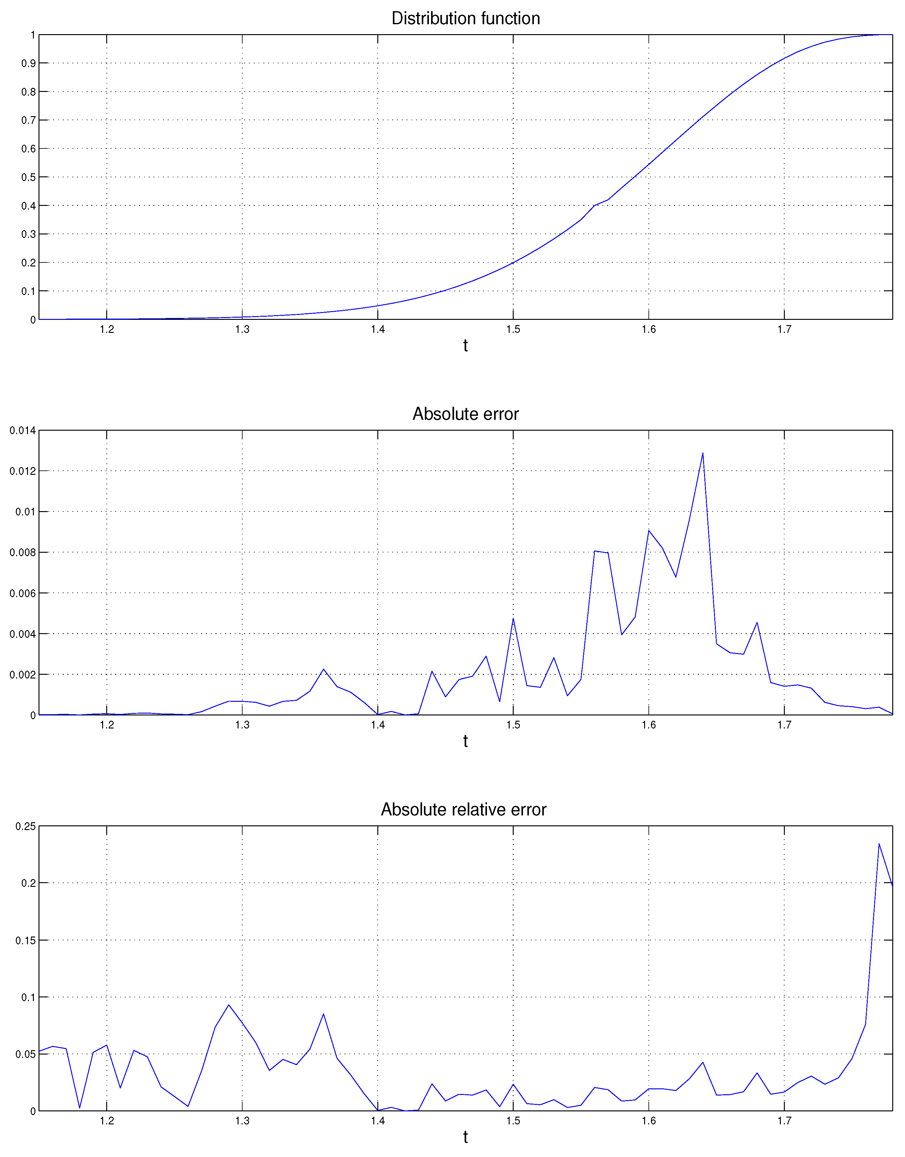
. The mathematical study of entropy began with Shannon [32], for the construction of a model for the transmission of information. In sampling with replacement from the urn, the probability of drawing a ball of color is fixed and given by , for . Define . The entropy of the coloration is given bywhere is assumed. The entropy is an appropriate measure of the uncertainty about the colors of the drawn balls. Indeed, it satisfies the following properties. First, takes its largest value for . Second, if we consider the equivalent coloration with probabilities and , respectively, then . Theorem 1 on pp. 9–10 of [33] states that the only continuous function that satisfies these two properties plus another one related to conditional entropy, has the form given in Equation (23) multiplied by a positive constant. As in Section 2.2, denotes the number of drawn balls for each of the n colors , respectively, after draws. Defineand that is, the multinomial probability of the configuration under uniformity. It is directly shown that Asymptotically, the entropy of the configuration is thus an increasing transform of the probability of the configuration under uniformity. The probability is maximized by the constant configuration and so is the entropy . Consider now the multinomial model in Equation (3) with unknown vector of probabilities . The frequency is an unbiased estimator of , for . Thus, is an estimator of the entropy . It takes the form of the M-statistic in Equation (1) with . Using the M-P representation and some algebraic manipulations, the c.g.f. in Equation (12) takes the formwith arbitrary. We set and select q such that , i.e., . With this choice of q, the marginal saddlepoint equation, cf. Equation (14), has the trivial solution . This yields Computing the second order derivatives is long but basic. We only give the simple result ; it can be used for controlling the formula of the second derivative.
We can now apply the saddlepoint approximation of Section 3 to the following case: , for , and . The saddlepoint approximation is compared with the Monte Carlo distribution of based on simulations. The numerical results are displayed in Figure 1 and Table 1. The probabilities obtained by simulation are denoted , the probabilities obtained by the saddlepoint approximation are denoted , denotes the absolute error defined in Equation (21) and denotes the absolute relative error defined in Equation (22), for . We see that the relative errors are mostly very small. The largest one occurs in the extreme right tail and it is around 31%. Example 2 (Power of likelihood ratio test)
. The estimator of entropy in Equation (24) is closely related to the likelihood ratio test. Consider a sample of k i.i.d. random variables and consider any partition of their range that is made by n intervals of positive length. Denote by the probability that any one of the sample values belongs to the jth interval, for . Denote by the number of sample values that belong to the jth interval, for . Then, takes values in and follows the multinomial distribution in Equation (3). Consider the null hypothesis , where . The likelihood ratio test statistic for against the general alternative is given by By restricting to , for some , we obtain In the case , which can be obtained without loss of generality by the probability integral transform, is equal to plus a constant term. Then, , as . In addition, if , with , for some , then is asymptotically normal.
The numerical evaluation of the saddlepoint approximation to the distribution of , with , and under , is given in Table 1 in [5]. We now extend the numerical study to the evaluation of the power function at any point of the alternative, viz. at any . Because is an affine transform of the entropy estimator given in Equation (24), we rather consider as test statistic. Thus, the c.g.f. for the saddlepoint approximation is already given in Equation (25). Consider the power function at the point of alternative hypothesis , for . We select and . The saddlepoint approximation to the distribution of under givesThe saddlepoint approximation to the distribution of under the chosen alternative point givesThis distribution is computed in Example 1. Thus, is the saddlepoint approximation to the power of the test with size 0.0495 at the given alternative. In situations where is the singleton containing the vector of unequal elements , the saddlepoint approximation can be obtained in a similar way. An important application is with language identification, where these probabilities represent the frequencies of the n letters of the alphabet of a language and are the frequencies of these n letters within a text of k letters. The belonging of the text to the language can be tested with the statistic , which is in fact proportional to the Kullback–Leibler information. Precisely, denotethe Kullback–Leibler information or discrepancy between the two probability distributions and , that satisfy the absolute continuity condition , for . Then, . Example 3 (Total claim amount under delayed settlement)
. We are interested in the distribution of the total claim amount of an insurance company over a fixed time horizon. We assume that the delay of claim settlement increases as the individual claim amount increases. This can happen in actuarial practice, partially because large claim amounts require longer controls. Precisely, the individual claim amounts are i.i.d. random variables taking the n values , all in , for . Let . Claims of amount are settled exactly after the jth unit of time (e.g., months). During a given time horizon (e.g., a year), claims of amount occur. We assume that claims have occurred during the time horizon under consideration and that , which takes values in , follows the multinomial distribution in Equation (3). The total claim amount settled during the time horizon is thus . We are interested in the distribution of the proportion of total claim amount that is settled exactly after the mth unit of time, viz. offor some . It can be re-expressed as the M-statistic in Equation (1) with The M-P representation tells that the multinomial claim counts have the distribution of independent Poisson occurrences, given a total of k claim occurrences. Thus, with some algebraic manipulations, the c.g.f. in Equation (12) becomeswith arbitrary . We set and select q such that , i.e., . Thus, the marginal saddlepoint equation, cf. Equation (14), is solved by . This leads to By computing the second order derivatives, we find .
For the numerical illustration, consider the multinomial distribution in Equation (3) with probabilities , , , , , , , and and the total number of claims. Thus, and the possible claim amounts are , , , , , , and . The number of unit of times for the proportion of settled total claim amount, cf. Equation (27), is . To assess the accuracy of the saddlepoint approximation, we compute the Monte Carlo distribution of , based on simulations. The numerical results are displayed in Table 2. The probabilities obtained by simulation are denoted , the probabilities obtained by the saddlepoint approximation are denoted and denotes the relative error, cf. Equation (22), for . Most relative errors are below 5%. The largest one occurs in the extreme left tail and is approximatively . A practical question would be the following: Which value of t bounds from above the proportion of total claim amount with probability 0.99? One computes directly and thus , approximately.
Example 4 (Bootstrap distribution of M-statistic)
. Let be a sample of i.i.d. random variables taking values in , for . Absolute continuity is assumed, in order to avoid repeated values a.s. Consider the M-statistic or defined as the root in t onwhere is continuous and decreasing in its second argument. Let be a realization of the sample and let be the random variables obtained by sampling with replacement from the values with respective probabilities , for . The distribution of , or simply , is the bootstrap distribution of . This coincides with sampling with replacement from the general urn model of Section 2.2, if the color is associated to the value , for , and if the number of draws from the urn is . Define , for , and for . Then, can be represented as the solution w.r.t. t of Equation (1), denoted , in which is the number of times that has been sampled, for . The conditional saddlepoint approximation of Section 3 yields the distribution of , i.e., of , i.e., of the bootstrap distribution of . In most practical cases, , i.e., . The saddlepoint approximation for bootstrap distributions was introduced by [34,35,36] and for M-estimators by [37]. A review can be found in [38] (Section 9.5). Thus, the conditional saddlepoint approximation of Section 3 provides an alternative saddlepoint approximation to the bootstrap distribution of M-estimators. Other applications of this saddlepoint approximation with the M-P representation that can be found the literature are the following. Saddlepoint approximations for likelihood ratio test and for chi-square tests for grouped data, under the null hypotheses, are given in [
3]. For the numerical evaluation of the saddlepoint approximation for the likelihood ratio statistic, refer to [
5].
4.2. Sampling without Replacement and MH-B Representation
The saddlepoint approximation combined with the MH-B representation can be applied for approximating the distribution of the M-statistic in Equation (
1) in finite population sampling, viz. under sampling without replacement. Example 5 analyzes the numerical accuracy of the saddlepoint approximation to the distribution of the coloration entropy when sampling is without replacement.
Example 5 (Entropy’s estimator under sampling without replacement)
. We consider the entropy estimation of Example 1 in the context of sampling without replacement. We are interested in the coloration entropy , as given by Equation (23), with unknown. It is the entropy of the initial state of the urn. In the multivariate hypergeometric model in Equation (4), is an unbiased estimator of , for , where takes values in . Thus, an estimator of this entropy is given by Equation (24). The unknown parameters of the multivariate hypergeometric distribution in Equation (4) are , for . With the MH-B representation and some algebraic manipulations, the c.g.f. in Equation (12) becomeswith arbitrary. We set and select q such that , i.e., . For this purpose, we assume . With this choice, the marginal saddlepoint equation, cf. Equation (14), has the trivial solution and the c.g.f. in Equation (28) becomes The second order derivatives of can be obtained through long but simple algebraic manipulations. In particular, we find .
For the numerical illustration, we consider the multivariate hypergeometric distribution with , , , , , , , and . We compute the Monte Carlo distribution of based on simulations. The saddlepoint approximation is obtained by following the steps of Section 3. The results are given in Table 3. The saddlepoint probabilities are obtained instantaneously and we see that the relative errors are below 15%, with the exception an extreme left tail point, for which the relative error is . We now summarize two practical applications of the conditional saddlepoint approximation with the MH-B representation. The first one can be found in [
39] and concerns a permutation test of comparison of two groups. The
jth individual belongs to the control group, when
, and to the treatment group, when
, for
. We have
, where
k is the number of individuals of the treatment group. The realizations of
represent the permutations of the individuals and the test statistic
is a linear combination of the elements of
. The permutation distribution of
is obtained from Equation (
2), where
are i.i.d. Bernoulli random variables.
The second application can be found in [
40] and concerns the jackknife distribution of a ratio. Consider the fixed sample
, sample without replacement
values and define
, if
is not sampled, and
, if
is sampled, for
. This procedure is repeated many times and a statistic of interest is computed
times, from the
k sampled values of each iteration. In the terminology of B. Efron, this is called the delete-
d jackknife. We have
, where
k is the sample size of the jackknife samples. The realizations of
represent the permutations of
. The statistic considered in [
40] is
, for
, for
. The permutation, viz. delete-
d jackknife, distribution of
is obtained from Equation (
2), where
are independent Bernoulli random variables with parameter
, together with the saddlepoint approximation for M-statistics of
Section 3.
4.3. Polya’s Sampling and MP-NB Representation
This section provides various applications of the saddlepoint approximation with the MP-NB representation. Example 6 considers the estimator of the entropy of the initial coloration probabilities of the urn, in the setting of Polya’s sampling. Example 7 considers the Bayesian analysis if this entropy. The Bayesian Entropy’s estimator under multivariate Polya a priori and sampling without replacement is considered. The saddlepoint approximation to this the posterior distribution of the entropy can be obtained by MP-NB representation. Example 8 concerns the saddlepoint approximation with the MP-NB representation for many two-sample tests based on spacing-frequencies.
Example 6 (Entropy’s estimator under Polya’s sampling)
. We consider the entropy estimation problem introduced in Example 1, now in the context of Polya’s sampling. We are interested in the entropy of the initial coloration probabilities , given in Equation (23), where are unknown. In the multivariate Polya model in Equation (5), is an unbiased estimator of , for , and so an estimator of the entropy is given by Equation (24). The parameters of the multivariate Polya distribution in Equation (5) are k equal to k of the urn model and , for . Using the MP-NB representation, the c.g.f. in Equation (12) becomeswith arbitrary. This formula allows for the direct evaluation of the conditional saddlepoint approximation of Section 3. Example 7 (Bayesian Entropy’s estimator under multivariate Polya a priori and sampling without replacement)
. The multivariate Polya distribution is often used as a prior distribution in Bayesian statistics, because it constitutes a conjugate class when associated to the multivariate hypergeometric likelihood. Precisely, consider the priortaking value in , for , and , and consider the likelihoodfor , and taking values in . Then, the posterior is given byfor . Indeed,where the last result is in fact equal to the posterior probability. Thus, Equation (31) holds. The underlying urn model is the sampling without replacement described, in Section 2.2, where the initial number of balls of each one of the colors , viz. , for , in the same order, is unknown. Only is known. These initial counts are the elements of the random vector with prior distribution in Equation (30). Sampling without replacement has led to the counts , for the colors , in same order. The updated or posterior distribution of is given by Equation (31). Assume that we are interested in the entropy of the probabilities of the initial coloration. The a priori entropy is thus , cf. Equation (23). According to Equation (31), the a posteriori entropy is , where . The saddlepoint approximations to the distributions of the a priori and a posteriori entropies can be obtained by the saddlepoint approximation of Section 3 with MP-NB representation, as in Example 6. The a priori and a posteriori c.g.f. can be obtained by minor adaptations of the c.g.f. in Equation (29). Example 8 (Two-sample tests based on spacing frequencies)
. Consider two independent samples: the first consisting of k independent random variables with common absolutely continuous distribution and the second sample consisting of l independent random variables with common absolutely continuous distribution . All these random variables have common range given by the real interval . We wish to test the null hypothesis . Define , and the ordered . Let . The random countsare called spacing-frequencies: they provide the number of random variables that lie between gaps made by . Thus, takes values in and possesses exchangeable components under . Denote by the rank of the jth largest in the combined sample, for . It is easily seen that , or, , for . Consequently, many two-sample test statistics based on ranks can be re-expressed in terms of spacing-frequencies. Besides this, spacing-frequencies are essential for the analysis of circular data, because they are invariant w.r.t. changes of null direction and sense of rotation (clockwise or anti-clockwise) (for a review, see, e.g., [41]). Circular data are planar directions and can be re-expressed as angles in radians, so that , or any other interval of length . Holst and Rao [42] consider nonparametric test statistics of the form offor some Borel functions . If , then the test statistic is called symmetric. Under , the multivariate Polya distribution in Equation (5) holds with . Consequently, and all Polya’s probabilities in Equation (5) are equal to . This is in accordance with the result of combinatorics that the number of solutions of the equation , i.e., card , is given by . Thus, the equivalence in Equation (2) holds with the MP-NB representation, where the negative binomial reduces to the geometric distribution. Clearly, Equation (33) takes the form of the M-statistic in Equation (1) and the saddlepoint approximation of Section 3 can be applied. We now summarize the examples presented in [3,5]. In the classical Wald–Wolfowitz run test, takes the symmetric form of Equation (33) with . We define a U-run in the combined sample as a maximal non-empty set of adjacent . Since each positive is mapped to a different U-run and conversely, yields the number of U-runs and it takes values in . Large values of show evidence for equal spread, i.e., for . [5] provides the numerical evaluation of the saddlepoint approximation to the distribution of under . The saddlepoint approximation to the distributions of the Wilcoxon viz. Mann–Whitney, the van der Waerden viz. normal score and the Savage viz. exponential score tests are developed in [3], The numerical study of Savage’s test appears in [5]. In the context of directional data, a generalization of Rao’s spacings tests (see Section 4.4) to spacing-frequencies together with the saddlepoint approximation is given in [41], which mention its saddlepoint approximation. The so-called multispacing-frequencies are obtained by gaps of order larger than one made by . Let denote the differentiation gap order, such that is an integer. Then, the multispacing-frequencies are defined by In the case , Equation (34) coincides with the spacing-frequencies in Equation (32). As before with , takes values in . We reconsider the null hypothesis and the general test statistics in Equation (33), however with the multispacing-frequencies in Equation (34). Under , the multivariate Polya distribution in Equation (5) holds with , and the MP-NB representation applies. The saddlepoint approximation with MP-NB representation was analyzed by Gatto and Jammalamadaka [7] in the context of the asymptotically most powerful multispacing-frequencies test against a specific sequence of alternative distributions and also in the context of the test statistic defined by the sum of squared multispacing-frequencies. It seems difficult to formulate an arbitrary alternative hypothesis in terms of a particular multivariate Polya distribution, for the multispacing-frequencies. In this sense, the conditional saddlepoint approximation with the MP-NB representation may not be easily applied to power computations.
4.4. D-G Representation
Example 9 of this section analyzes the most powerful test of symmetry of the Dirichlet distribution. The saddlepoint approximation based on the D-G representation to the distribution of the test statistic under an asymmetric alternative is developed and its numerical accuracy is studied. The Dirichlet associated to the multinomial distribution is an important conjugate class of distributions in Bayesian statistic. This is illustrated in Example 10, which presents a Bayesian bootstrap test on the entropy. The D-G representation with the conditional saddlepoint approximation allow to compute the Bayes factor of the test, without resampling. Another important application of the saddlepoint approximation with the D-G representation is for the class of one-sample tests based on spacings. This class of nonparametric tests is presented in Example 11 and has some similarities with the two-sample tests based on spacing frequencies of Example 8. Example 11 provides a summary of the applications that can be found in the literature of this saddlepoint approximation to tests based on spacings.
Example 9 (Test for Dirichlet’s symmetry)
. The symmetric Dirichlet distribution is obtained by setting in Equation (9), for any . In Bayesian statistics, symmetric priors are of particular interest in absence of prior knowledge on the individual elements, because they become exchangeable random variables. The single parameter a becomes a concentration parameter: yields the uniform distribution over (thus, the noninformative prior); yields a concave density over (thus, promoting similarity of elements); and yields a convex density over (thus, promoting dissimilarity of elements). For , consider the testing problem of a particular symmetry against any particular asymmetric alternative. Precisely, given , where at least one the values differs from the other ones, consider , against . The test of uniformity is obtained with . Neyman–Pearson’s Lemma tells that the most powerful test has the form , where viz. is given by It is the M-statistic in Equation (1) with , for . From the D-G representation and some algebraic manipulations, the c.g.f. in Equation (12) becomeswhere and arbitrary. We set and select q such that , i.e. . The marginal saddlepoint equation, cf. Equation (14), has then as solution. This leads to The second order derivatives of can be expressed in terms of polygamma functions , for . We skip the details but note that .
In the following numerical illustration, and , for , so . The saddlepoint approximation is computed under , so it gives the power of the test. It is compared with the Monte Carlo distribution of with simulations. The numerical results are displayed in Table 4. The probabilities obtained by simulation are denoted , the probabilities obtained by the saddlepoint approximation are denoted and denotes the absolute relative error given in Equation (22), for t in the lower and in the upper tails of the distribution. The relative errors of both lower and upper tails do not exceed . Example 10 (Bayesian bootstrap and Bayesian entropy test)
. In Bayesian statistics, Dirichlet and multinomial distributions are conjugate: Dirichlet prior and multinomial likelihood lead to Dirichlet posterior. Precisely, ifandthen and . The Bayesian bootstrap was introduced by Rubin [43] as a method for approximating the posterior distribution of a random parameter; precisely the distribution of a function of , given the observed data . It consists in sampling of from Equation (38). This can be done by generating Gamma
, for , independently, and by setting The value of is irrelevant. Details can be found in Section 10.5 of [38]. Assume that the parameter of interest is that admits the M-statistic representation in Equation (1), then the saddlepoint approximation with the D-G representation can be used instead of the described sampling method. Consider now the urn model of Section 2.2 with sampling with replacement, where the probability of drawing a ball of color is given by the random variable , for . We are interested in the entropy , viz. Equation (23) as a function of . According to Equation (10), is the entropy of the sample proportions of colors under Polya’s sampling at steady state. Thus, , for ; cf. Section 2.3. We consider the Bayesian testing problem , against , for some . Then, and are the prior probabilities of and , respectively. Their analog posteriors are and , where and . The Bayes factor of to is the posterior odds ratio over the prior odds ratio , namely . The Monte Carlo solution consists in sampling of from the prior in Equation (37) and then from the posterior (38), both levels by means of Equation (39). Thus, and are Bayesian bootstrap estimators of and , respectively, and they allow for the evaluation of . Alternatively, these values can be obtained without repeated sampling by using the conditional saddlepoint approximation of Section 3 with the D-G representation. Example 11 (Tests based on spacings)
. The so-called spacings are the first order differences or gaps between successive values of the ordered sample. Let be absolutely continuous and i.i.d. over , without loss of generality by the probability integral transform, let denote the ordered sample and let and . For , the spacings are defined by Thus, takes values in . Statistics that are defined as functions of spacings are used in various statistical problems, goodness-of-fit testing representing the most important (see, e.g., [44]). Spacings are essential in the analysis of circular data, because they form a maximal invariant w.r.t. changes of null direction and sense of rotation. For Borel functions , for , important spacings statistics have the form If , then the test statistic is called symmetric. Under the null hypothesis of uniformity of , the D-G representation holds with , so that the n spacings are equivalent in distribution to n i.i.d. exponential random variables conditioned by their sum. As Equation (41) takes the form of the M-statistic in Equation (1), the saddlepoint approximation of Section 3 can be directly applied. The conditional saddlepoint approximation with the D-G representation under is analyzed numerically by [3] in the following cases: Rao’s spacings test (viz., , for ), the logarithm spacings test (viz., , for ), Greenwood’s test (viz., , for ) and a locally most powerful spacings test (viz., , for ). In the context of reliability, Gatto and Jammalamadaka [6] re-expressed a uniformly most powerful test of exponentially, against alternatives with increasing failure rate, in terms of spacings. They obtained the saddlepoint approximation and show some numerical comparisons. These spacings can be generalized to higher order differences or gaps. Let denote the gap order, selected such that . The so-called multispacings are defined as As previously, takes values in . When , the random variables in Equation (42) coincide with the spacings in Equation (40). Under , the D-G representation holds with . Gatto and Jammalamadaka [7] provided explicit formulae of the saddlepoint approximations for Rao’s multispacings test and for the logarithmic multispacings test, together with a numerical study. The next problem would be the computation of the distribution of a spacings or multispacings test statistic under a non-uniform alternative distribution. This can be done by saddlepoint approximation with the D-G representation whenever one can find the parameters such that, under the alternative distribution, the spacings or multispacings satisfy Dirichlet(). This would give the power of the test. However, re-expressing a non-uniform distribution in terms of a particular Dirichlet distribution does not appear practical, in general.
5. Final Remarks
This article presents the saddlepoint approximation for M-statistics of dependent random variables taking values in a simplex. Four conditional representations that allow re-expressing these dependent random variables as independent ones are presented. A detailed presentation of the underlying urn sampling model that is common to all four conditional representations is given. Important applications are reviewed. New applications are presented with some numerical comparisons between this saddlepoint approximation and Monte Carlo simulation. The numerical accuracy of the saddlepoint approximation appears very good.
A practical question concerns the relative advantages and disadvantages of using the conditional saddlepoint approximation presented in this article. Indeed, tail probabilities can be computed rapidly and more easily by means of Monte Carlo simulation. However, there is no unique answer to this general question, because several aspects should be considered.
First, when very small tail probabilities, e.g.,
, or extreme quantiles are desired, then the simple Monte Carlo used in this article may not always lead to accurate results. The reason is that the saddlepoint approximation is a large deviation technique, with bounded relative error everywhere in the tails, whereas simple Monte Carlo has unbounded relative error in the tails. In fact, simple Monte Carlo is even not logarithmic efficient. This is well explained in [
45] (pp. 158–160). To have bounded relative error, importance sampling is required. Then, the mathematical complexity would become close to the one of the saddlepoint approximation. Moreover, computing quantiles by importance sampling may not be straightforward. As shown above, this is quite simple with the saddlepoint approximation.
The computations required for this article were done with
Matlab (R2017b, The MathWorks, Natick, MA, USA). The minimization program
fminsearch was used for obtaining the saddlepoint defined in Equation (
13). All
Matlab programs are available at
http://www.stat.unibe.ch. They should be easily used and modified for new related applications.
One should also mention that, having analytical expression such as a saddlepoint approximation for computing a quantity of interest, may have advantages. Monte Carlo and other purely numerical methods often do not provide such an expression. For example, the saddlepoint approximation can be used for computing the sensitivity of the upper tail probability, viz. the derivative of the tail probability w.r.t. to a parameter of the model. Gatto and Peeters [
46] proposed evaluating the sensitivityof the tail probability of the random sum w.r.t. the parameter of the summation index distribution (which is either Poisson or geometric) with the saddlepoint approximation. They showed numerically that the sensitivities obtained by the saddlepoint approximation and by simulation with importance sampling are very close, but this no longer true when simulation is without importance sampling. In the case of computing sensitivity, importance sampling is significantly more computationally intensive than the saddlepoint approximation.
An application of the saddlepoint approximation that exploits a different conditional representation concerns the distribution of the inhomogeneous compound Poisson total claim amount under force of interest, in the context of insurance. It was suggested by [
47] and the main idea is the following. The inhomogeneous Poisson process of occurrence times of individual claims is given by
. Let
denote the number of occurrences during the time interval
, for some
. Then,
,
where
are the ordered values of some random variables
that are nonnegative, i.i.d. and independent of
. The individual claim amounts are represented by the random variables
that are nonnegative, i.i.d. and independent of
. Let
denote the force of interest. The discounted total claim amount is
, for
, and Equation (
43) implies
, for
. The last random sum has a simple structure and its distribution can be computed by the saddlepoint approximation of [
18].
A technique that could exploit the four conditional representations of
Section 2 for computing the conditional c.g.f. (and not the conditional saddlepoint approximation) can be found in [
48]. It is tentatively applied, with the MP-NB representation, to the symmetric spacing-frequencies test statistic in Equation (
33) in [
41] (Section 6.3.2). However, this approach seems impractical.
Another extension of the proposed approximation would concern neutrosophic statistics. In standard statistics, observations and parameters are represented by precise values, whereas in neutrosophic statistics they remain indeterminate (see, e.g., [
49]).


