Using Various Models for Predicting Soil Organic Carbon Based on DRIFT-FTIR and Chemical Analysis

Abstract

Soil organic carbon (SOC) is a crucial factor influencing soil quality and fertility. In this particular investigation, we aimed to explore the possibility of using diffuse reflectance infrared fourier transform spectroscopy (DRIFT-FTIR) in conjunction with machine-learning models, such as partial least squares regression (PLSR), artificial neural networks (ANN), support vector regression (SVR) and random forest (RF), to estimate SOC in Sohag, Egypt. To achieve this, we collected a total of ninety surface soil samples from various locations in Sohag and estimated the total organic carbon content using both the Walkley-Black method and DRIFT-FTIR spectroscopy. Subsequently, we used the spectral data to develop regression models using PLSR, ANN, SVR, and RF. To evaluate the performance of these models, we used several evaluation parameters, including root mean square error (RMSE), coefficient of determination (R²), and ratio of performance deviation (RPD). Our survey results revealed that the PLSR model had the most favorable performance, yielding an R² value of 0.82 and an RMSE of 0.006%. In contrast, the ANN, SVR, and RF models demonstrated moderate to poor performance, with R² values of 0.53, 0.27, and 0.18, respectively. Overall, our study highlights the potential of combining DRIFT-FTIR spectroscopy with multivariate analysis techniques to predict SOC in Sohag, Egypt. However, additional studies and research are needed to improve the accuracy or predictability of machine-learning models incorporated into DRIFT-FTIR analysis and to compare DRIFT-FTIR analysis techniques with conventional soil chemical measurements.

1. Introduction

SOC is the main factor influencing soil quality, fertility, agricultural economic viability, and sequestration of atmospheric carbon dioxide (CO₂). The presence of SOC modifies the physical, chemical, and biological properties of the soil, resulting in improved soil water and nutrient retention [1] as well as improved soil health and sustainability [2]. SOC plays a crucial role in carbon sequestration and climate change mitigation [2].

The range of SOC can differ depending on various factors such as soil type, land management practices, and vegetation cover [3]. SOC levels below 1.5% are considered low and may indicate long-term degradation, limited organic matter inputs, or intensive cultivation without appropriate organic matter management [1]. On the other hand, SOC levels ranging from 1.5% to 3% are considered moderate and suggest reasonably good organic matter content, reflecting adequate organic inputs and appropriate land management practices [4].

Accurate determination of SOC is of immense importance in formulating effective land management tactics, environmental regulations, climate change mitigation plans, and conservation methodologies aimed at increasing soil carbon sequestration [5,6]. It provides vital information for understanding and monitoring soil health, carbon sequestration potential, and sustainable land use practices [7,8,9,10].

There are various common techniques available for determining SOC, including Walkley-Black and dry elemental analysis methods. However, the Walkley-Black method is commonly used in routine soil-testing laboratories due to its widespread adoption [11]. However, this method is known to be time-consuming, laborious, expensive, and environmentally hazardous [12]. On the other hand, near-infrared spectroscopy (NIRS) and mid-infrared spectroscopy (MIRS) are rapid and non-destructive techniques that exploit the spectral properties of soil samples to estimate SOC content [13]. These advanced techniques provide faster results and can be applied in the laboratory, in situ, or during large-scale investigations [14].

The use of DRIFT-FTIR spectroscopy and other advanced techniques to estimate SOC aligns with the principles of precision agriculture, which involves the implementation of site-specific management practices based on soil variability [15]. By examining the spectral patterns of soil samples, DRIFT-FTIR spectroscopy can offer valuable insights into the spatial distribution of SOC content in a field. One of the main advantages of DRIFT-FTIR spectroscopy is its ability to provide accurate and rapid SOC determination, as previously studied by [16,17], typically requiring only a few minutes per sample. This efficiency allows for high sample throughput, making it well-suited for large-scale studies or monitoring programs where time efficiency is crucial [18]. Additionally, DRIFT-FTIR spectroscopy facilitates the monitoring of carbon sequestration efforts for sustainable agriculture and climate change mitigation [6].

DRIFT-FTIR spectroscopy is a non-destructive method, which means that soil samples remain intact and can be used for later analyzes or for archiving. DRIFT-FTIR spectroscopy can provide accurate estimates of SOC content when properly calibrated and validated [19]. The technique uses the specific infrared absorption characteristics of soil organic functional groups, allowing quantification of SOC with good accuracy over a wide range of SOC values, from low to high levels [20]. However, the accuracy and precision of the determination may vary within this range. DRIFT-FTIR spectroscopy is particularly effective for estimating SOC levels between 1% and 10% (w/w) or higher [21]. This range covers typical SOC levels found in agricultural soils and can be reliably detected using well-developed calibration models and appropriate sample analysis techniques. The presence of gypsum and limestone can have an impact on the level of SOC. Adding limestone to soil as a liming agent can significantly increase plant biomass above and below ground, which increases carbon yield [22]. Additionally, the presence of limestone in the soil can increase soil pH, which will impact microbial activity and soil carbon sequestration [23,24]. A significant amount of terrestrial carbon can be stored in gypsum soils, preventing it from being released as carbon dioxide, the main greenhouse gas, into the atmosphere [25]. The application of gypsum can continuously dissolve organic carbon, leading to higher organic carbon content compared to unchanged controls [26].

In some cases, DRIFT-FTIR spectroscopy can detect SOC content as low as 0.5% or less, but this may require careful calibration and validation. It is important to note that the lower detection limits of the DRIFT-FTIR determination of SOC may depend on factors such as soil mDRIFTix, the presence of interfering substances, and instrument sensitivity. Additionally, extremely high SOC contents (>30% or more) can pose problems in terms of spectral saturation, where absorption bands associated with SOC become saturated, making accurate quantification more difficult [19]. Certain soil characteristics affect the DRIFT-FTIR analysis, such as soil moisture (by changing the water absorption bands), pH (extreme values of soil pH [very acidic or alkaline] can affect spectral properties of organic compounds and reduce analysis accuracy estimation of SOC), texture (some textures, such as clay-rich soils, may exhibit higher spectral noise due to increased interference from clay minerals), clay minerals, and iron oxides (overlapping absorbances of these minerals can facilitate the interpretation of spectra for SOM characterization) [4]. These influence the accuracy of prediction models [27].

To eliminate the effect of soil moisture on the FTIR spectra, all soil samples were oven dried at the same temperature for the same time. On the other hand, to solve the problem of the effects of several soil parameters, such as pH, texture, minerals, oxides, etc., there are certain procedures which can be described as follows.

(i)

Sample preparation was carried out uniformly and one procedure was used for sample collection, storage, and analysis.

(ii)

Spectral preprocessing techniques, such as normalization to FTIR spectra, can help reduce noise and variability in spectra, thereby facilitating the identification and interpretation of organic carbon bands.

(iii)

Using calibration models of PLSR, ANN, RF, and SVR can help correlate FTIR spectra with SOC content while considering the effect of other soil parameters.

(iv)

Standardization of FTIR measurements, including calibration of instruments to ensure that the data collected is reliable and consistent for different soil parameters.

The correlation between DRIFT-FTIR data and soil organic carbon (SOC) content is established through the absorption of infrared radiation in the mid-infrared range (4000–400 cm⁻¹) by the organic functional groups present in the ground [19]. The infrared spectrum contains unique absorption bands for different functional groups, such as aliphatic compounds, aromatic compounds, and carboxylic acid groups. Chemical bonds exhibit distinct vibrational movements, including stretching, bending, and deformation, specific to each molecule. DRIFT-FTIR spectroscopy measures the molecular vibrations of organic compounds, producing a spectral fingerprint that can be used to estimate SOC content [28,29]. The calibration process involves the analysis of a set of soil samples with known SOC content (determined by traditional laboratory chemical methods) using DRIFT-FTIR spectroscopy [19]. The transmission data, usually represented as a spectral curve, is then correlated with the corresponding SOC content of each sample. This information is then used to build calibration models that establish the relationship between reflectance and SOC content. The correlation between the reflectance data is usually represented as a spectral curve, and the corresponding SOC content of each sample is used. This information is then used to build calibration models that relate reflectance data to SOC content. Once these calibration models are developed, reflectance data acquired from unknown soil samples can be input into the models to estimate SOC content [15]. The spectral information is used by the models to correlate with the known SOC content obtained from the calibration samples. This correlation allows quantitative estimation of SOC levels in unknown samples by analyzing their infrared spectra. The accuracy of this estimate depends on the quality and representativeness of the calibration data set. To assess the accuracy and reliability of calibration methods, cross-validation techniques such as splitting the dataset into training and validation sets or using independent validation samples are used [30].

Several machine-learning models can be used to estimate SOC using DRIFT-FTIR data. The choice of model depends on factors such as characteristics of the dataset (homogeneity and size), sample size (a large sample size is suitable for complex models while a smaller sample size is suitable for simple models), feature selection, and desired interpretability. Among these models, PLSR, SVR, RF, and ANN models can be used to predict SOC using DRIFT-FTIR spectra. These machine-learning models are described as follows:

1.1.

PLSR is a widely adopted regression technique for analyzing spectroscopic data, including DRIFT-FTIR. It identifies latent variables in the data and establishes a linear relationship between these factors and the targeted variable (SOC). PLSR is particularly suited to the processing of collinear and high-dimensional spectral data [18].

1.2.

SVR is a popular machine-learning algorithm that maps DRIFT-FTIR spectral data to SOC values while aiming to maximize the error tolerance margin. It can effectively handle nonlinear relationships and has the potential to provide accurate predictions [15].

1.3.

RF regression is an ensemble learning method combining multiple decision trees to provide predictions. It can handle complex relationships between variables, handle high-dimensional data, and has built-in feature importance ranking, which can help identify the most relevant spectral features for SOC estimation [31].

1.4.

ANN models, such as feed-forward neural networks, can capture complex nonlinear relationships between spectral features and SOC. By training on the DRIFT-FTIR dataset, ANNs can learn patterns and make predictions based on spectral information [20].

Model effectiveness is influenced by various factors, including the caliber and relevance of training data, feature engineering methods, hyperparameter tuning, and cross-validation approaches. Accordingly, it is advisable to study and compare the performance of distinct models on particular datasets to identify the optimal model for SOC estimation using DRIFT-FTIR data.

The effectiveness of PLSR, ANN, RF, and SVR machine-learning models has been widely studied in recent research for estimating and predicting SOC using DRIFT-FTIR data. The R-squared (R²) value, which is commonly used to evaluate the accuracy of SOC prediction, can vary depending on various factors such as the calibration dataset, complexity of the soil system, quality spectral data, and the calibration model used. It is difficult to provide an accurate R² value as it can differ significantly between different studies. However, in general, R² values for SOC prediction in calibration models using DRIFT-FTIR spectroscopy typically range from 0.7 to 0.9 or higher [18,20]. However, relying solely on the R² value may not fully account for the effectiveness or reliability of the calibration model. It is advisable to consider additional statistical measures such as root mean square error (RMSE), bias, or validation measures to comprehensively evaluate the accuracy and predictive performance of SOC estimates using the DRIFT-FTIR spectroscopy [20,32,33]. Goydaragh et al. [16] predicted the SOC content of some Iranian soils using DRIFT-FTIR. They found that the Cupist and Bat machine-learning models performed well for prediction with an R2 of 0.77 and RMSE of 0.28. Xu et al. [34] used DRIFT-FTIR-DRIFT data to predict SOM in some Chinese soils with reasonable performance while the R² values of PLSR, SVR, and CNN were 0.701, 0.643, and 0.635, respectively. Veum et al. [35] used PLSR combined with MIR ground data to predict SOC with an R² of 0.69, while they predicted SOC using VIS-NIR with an R² = 0.94. Calderon et al. [36] obtained good predictability of SOC using MIR data and the PLSR model, while the prediction R² was 0.81. Margenot et al. [37] used the ANN model with DRIFT-FTIR spectra to predict SOC. They found that the R² of the ANN validation was 0.92 with RMSE = 0.35.

The choice of significant bands in DRIFT-FTIR spectral data for SOC estimation or prediction varies depending on the specific research studies and calibration models used. The selection of these bands can be influenced by the presence of organic functional groups in the MOS. However, some general regions and bands in the mid-infrared range (4000–400 cm⁻¹) have been identified as useful for SOC prediction using DRIFT-FTIR spectroscopy, as reported in [16,38,39,40]. Specifically, C-H stretching vibrations are associated with bands between 2950 and 2800 cm⁻¹, which correspond to aliphatic (saturated) hydrocarbons.

The spectral region between 1750 and 1660 cm⁻¹ is attributed to the stretching vibrations of the C=O bond, which can be attributed to various carbonyl functional groups such as ketones, esters, or carboxylic acids [41]. The presence of O–H stretching vibrations originating from hydroxyl (OH) groups can be inferred from the bands observed in the range of 3500–3000 cm⁻¹. C–O stretching vibrations originating from C–OH or C–O–C functional groups are represented by bands on the order of 1200 to 1000 cm⁻¹. Aromatic compounds can be associated with bands observed from 1600–1490 cm⁻¹. Baes and Bloom [42] reported that the weak band near 1550 cm⁻¹ in the black soil spectra can be attributed to the aromatic C=C vibration, which reveals the distinctive structure of organic matter in the soil.

In Egypt, traditional methods of soil analysis are used. These methods are quite expensive due to the high price of chemicals. Additionally, these methods are laborious and time-consuming. Additionally, such studies or research are lacking in Egypt, as it is difficult to find similar work on using DRIFT-FTIR to estimate SOC.

The research deficiency lies in the fact that previous studies on Sohag soils failed to conduct a comparative analysis of various machine-learning models with the aim of estimating SOC using the data DRIFT-FTIR. Accordingly, this study aims to fill this gap by using several machine-learning models, including PLSR, ANN, RF, and SVR, to predict SOC in agricultural soils located in Sohag, Egypt, as a representative of alluvial soils. The ultimate goal is to identify the most efficient prediction model that can be used to estimate SOC based on DRIFT-FTIR data.

Based on the previous introduction, the main objective of this study is to predict SOC using the DRIFT-FTIR technique alongside various prediction models (PLSR, ANN, RF, and SVR). These models will be used to analyze soil samples obtained in the Sohag region of Egypt.

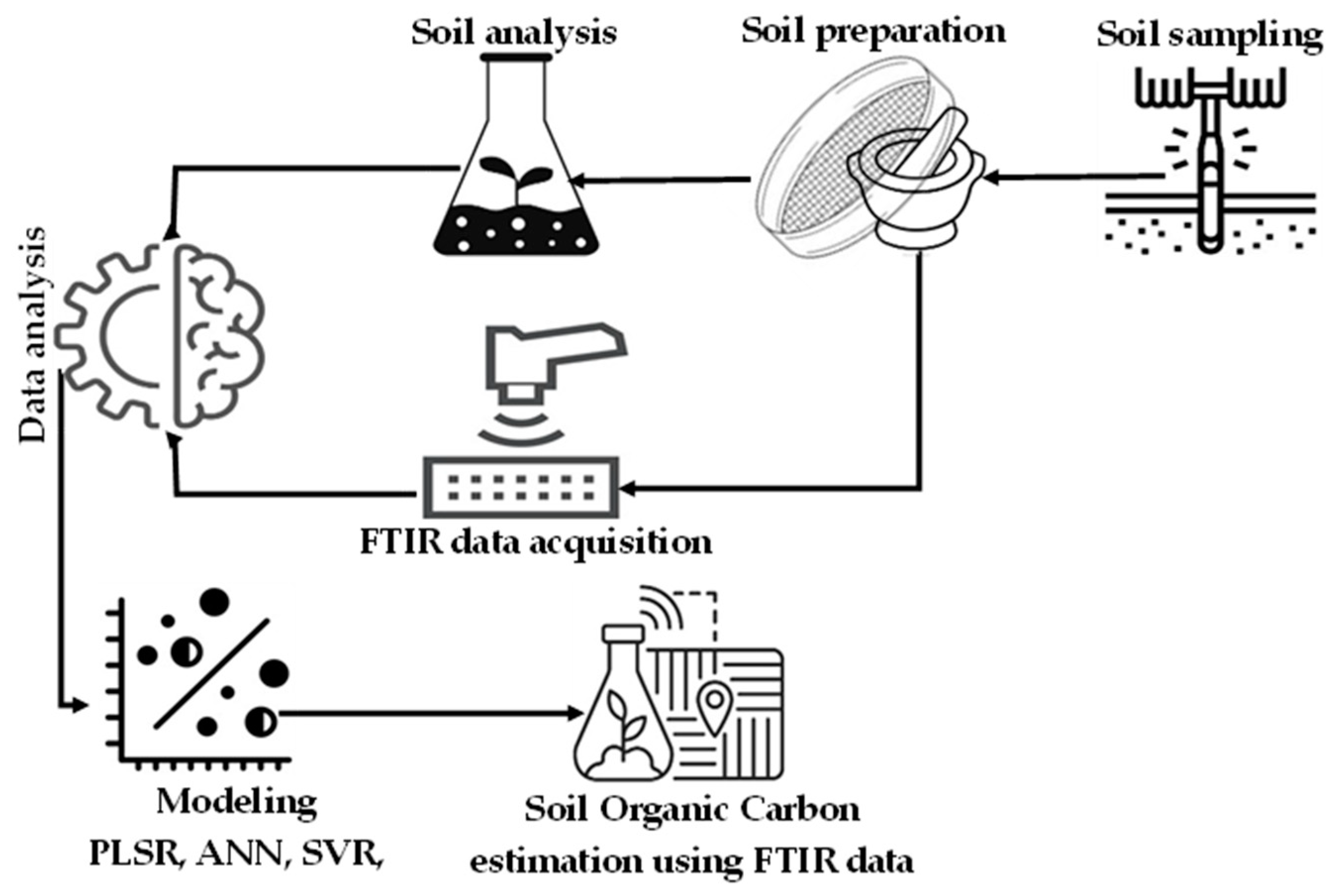
2. Materials and Methods

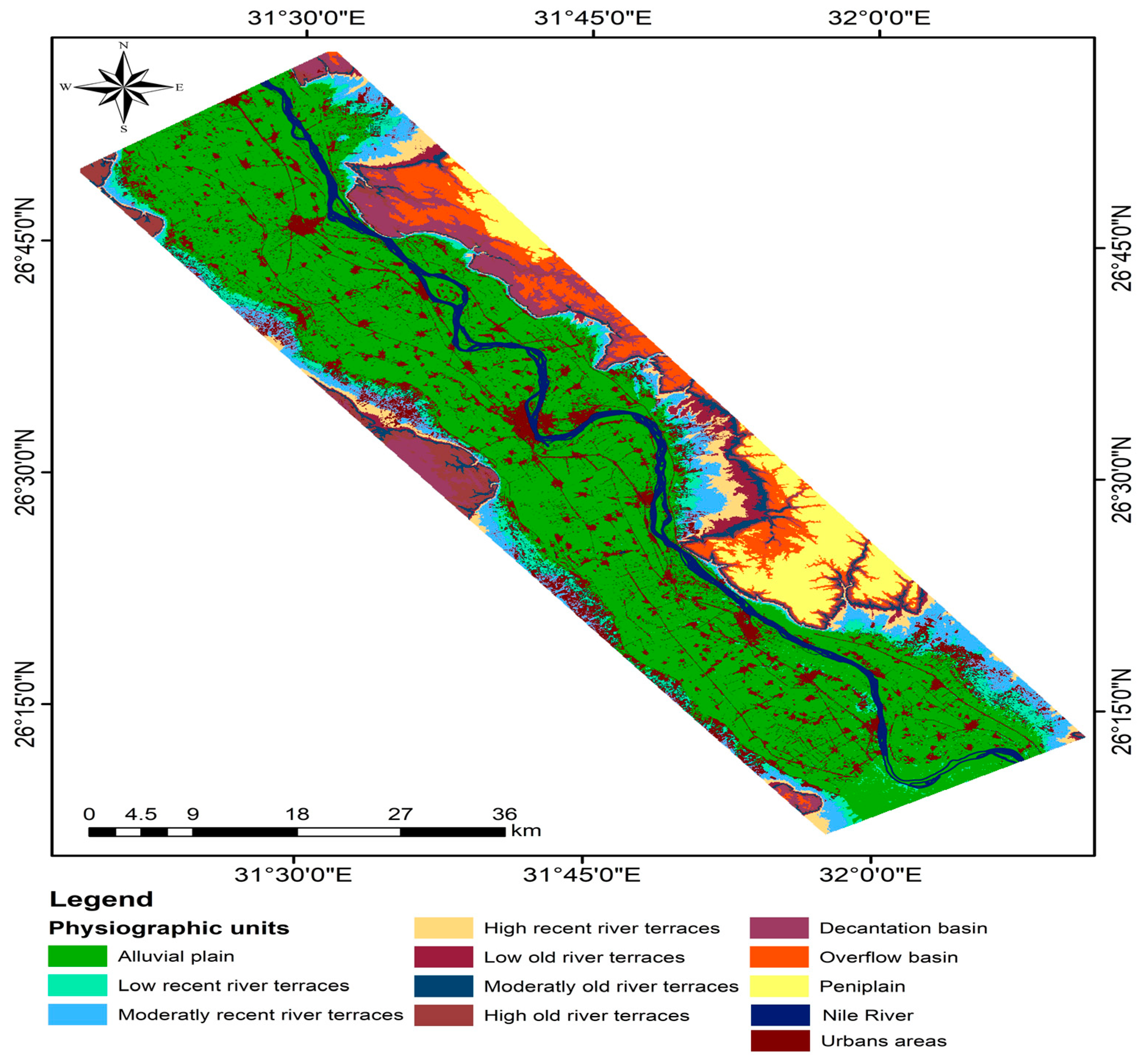
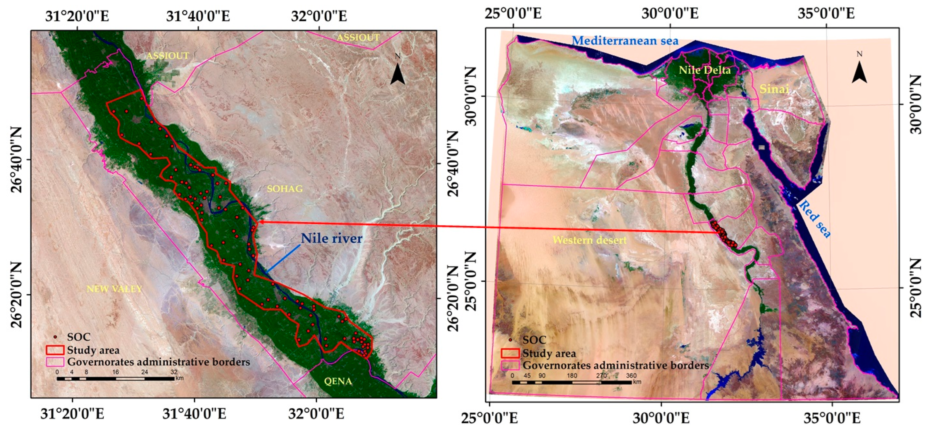
The methodology employed in this study is illustrated in Figure 1. The methodological framework included a series of steps from the collection of soil samples to their preparation, followed by SOC analysis using the conventional chemical method (Walkley-Black method); DRIFT-FTIR data acquisition; data processing; modeling using various models such as PLSR, ANN, SVR, RF; and SOC estimation using DRIFT-FTIR data, respectively.

2.1. The Study Area

The region examined encompasses part of Sohag Governorate, stretching from the town of Tima in the north to the town of El-Baliana in the south. It mainly includes historic agricultural fields located in the Nile Valley as well as recently reclaimed lands. The search area is located between latitudes 26°10′21.28″ and 26°50′30.95″ N and longitudes 31°20′51.45″ and 32°09′49.11″ E, with elevations ranging from 61 to 73 m above sea level. A map illustrating the study region can be found in Figure 2. This research area is located in North Africa, known for its hot summers, mild winters, and limited rainfall. The air temperature in this region fluctuates between 36.5 °C in summer and 15.5 °C in winter. Relative humidity ranges from 51 to 61% in winter, 33 to 41% in spring, and 35 to 42% in summer. Weather data for the year 2022 relating to the study area were obtained from the website (https://weatherspark.com/ (accessed on 13 July 2022)). In Sohag Governorate, cultivated alluvial areas extend along the banks of the Nile. The Nile is the main source of irrigation for existing agricultural soils, while groundwater supplies irrigation to some areas of recently reclaimed land.

The research site includes an alluvial plain, which is ancient cultivated agricultural soil. The majority of these soils have a dense texture, with clay being the main component, and moderate drainage. The study area generally cultivates a variety of crops, such as wheat, corn, alfalfa, sorghum, beans, tomato, potato, pepper, eggplant, onion, and others. During field sampling visits, some concerns were identified, including salinity in some areas caused by the intensive use of chemical fertilizers and soil degradation due to urban sprawl on agricultural fields.

2.2. Soil Sampling

Based on the generated physiographic map of Sohag Governorate, there are 12 physiographic units, as shown in Figure 2. The studied soils were located in the alluvial plain. Ninety soil samples from the surface layer (0–30 cm) were obtained vertically (North and South) across the study area, as shown in Figure 3. These soils were classified up to the level of great group level according to the world reference base (WRB) soil classification [43]. These soils belonged to the order Entisols [44].

The selection of sampling sites was based on the spatial heterogeneity observed in the alluvial soil. To account for the variability present across the area, a random sampling approach was used. This involved collecting soil samples from random locations within the designated sampling area. The study area included two distinct land uses: cultivated soils and uncultivated soils (soils after harvest of previous crops). Soil samples from uncultivated soils were collected following the harvest of previously cultivated crops. It is important to note that soil sampling took place during the summer of 2022, ensuring the absence of any plant residue. The WGS-1984 coordinate system was used to accurately record the latitudes and longitudes of the soil sampling sites using a GPS device (Garmin e-trix Kansas, USA) in the field. Aslan-Sungur et al. [45], Goydaragh et al. [16], and Tiruneh et al. [46] collected a similar number of samples for SOC prediction based on DRIFT-FTIR spectra and the same models used.

2.3. Soil Samples Preparation and Analysis

The collected soil samples were subjected to an air-drying process for three days at a room temperature of 40 ± 2 °C. During this time, all visible plant roots, rocks, and debris were carefully removed. Subsequently, the dried soil samples were crushed using a wooden mortar and then passed through a 2 mm sieve. In order to characterize the collected soil samples, routine soil analysis was carried out. Soil pH was measured using a pH-meter equipped with a glass electrode, including the pH 211 microprocessor pH-meter manufactured by HANNA Instruments (Leighton Buzzard, United Kingdom). This measurement was carried out on a soil/water suspension in a ratio of 1:2.5. To determine the electrical conductivity (EC) of the soil, an electrical conductivity meter known as Orion Model 150 (USA) from the United States was used. The EC measurement was carried out on an extract obtained from a soil/water ratio of 1:2.5. The particle size distribution of the soil was determined using the international pipette method referenced in [47,48]. Soil fractions (sand, silt, and clay) were calculated based on the mentioned method. The total calcium carbonates present in the soil were estimated volumetrically using the Colins’ calcimeter (USA)as mentioned in [49]. Soil organic carbon (SOC) content was determined by the wet oxidation method known as the Walkly and Black method, as described in [48].

2.4. Spectral Data Acquisition

To obtain ground spectral data, the methodology described by Margenot et al. [50] was followed. The prepared soil samples were ground again, then passed through a 0.2 mm sieve and oven dried at 60 °C overnight to remove moisture OH groups. Then, the sieved samples were scanned using the Bruker Alpha Platinum-DRIFT-FTIR spectrometer (Germany), covering the spectral range of 4000 to 400 cm⁻¹ of the wavenumber region, with a resolution of a wavenumber interval of 4 cm⁻¹. This analysis was performed using KBr pellets as the output of the device in transmission form. The resulting soil spectral signatures, acquired in transmission format from the DRIFT-FTIR spectrometer, were converted to text format using Origin-pro software version 8.0.63.988. This conversion facilitated the processing and sharing of the data with other software packages.

Table 1. The significant bands in the DRIFT-FTIR spectra of soil or some similar substrates and their assignments.

Wavenumber (cm−1)	Functional Group	Substrate	Assignment	Reference
3696, 3622, 3620	Si–O-H–vibrations	Soil	Clay minerals, gibbsite, Fe oxides	[51,52,53]
3640–3610/3420–3400	O–H stretching	Soil/peat	Alcohols and phenols	[54,55]
3246	H-bonded OH	Soil	Humic acid	[56]
3000–2800	C–H stretching	Lignite	aliphatic methylene groups	[57]
2941, 2922, 2885, and 2850	methyl C–H stretching	Soil	aliphatic compounds	[1]
2925–2855	asymmetric stretching of CH3 and CH2	Soil, Peat	Methyl and Methylene	[55,58]
1725–1710	C=O stretching	Peat	carboxylic acids	[55]
1760–1690, 1640, 1644,1648	C=O stretching and COO-	Soil	carboxylic acids	[56,59]
1600–1500/1625–1610	C=C stretching	Lignite/Peat	aromatic compounds	[55,60]
Around 1584	C=O stretching	Soil	carboxylic acids	[58]
1540	C–N stretching or N–H bending vibrations	Soil	amide groups	[61]
1433–1427, 1420–1425	C–O	Soil	carbonate minerals	[53,62,63]
1420, 1380/1370	C–H	Peat/Soil	Methoxyl and methyl/ C–H absorption in aliphatics, CO–CH3 vibrations in lignin- derived phenols	[53,64,65,66]
1200–1300	C–O stretching	Soil	carbohydrates, cellulose, and hemicellulose	[19]
1270 and 1235	C–O stretching	Peat	Phenolic group and aromatic ethers	[67]
1060–1010	Al–OH Deformation or C–O stretching	Soil	Kaolinite or polysaccharide groups	[53]
1033–1030	Si–O–Si, Si–O stretching	Soil	Clay minerals or quartz	[50]
915	Al–OH	Soil	Kaolinite and smectite minerals	[68,69,70]
870–890	C–O	Soil	carbonate minerals	[53]
779, 780, 690–695, 468	Si–O	Soil	Quartz	[52]
537–539	Al–O deformation	Soil	Kaolinite mineral	[71]

shows the significant bands that were observed in the DRIFT-FTIR spectra in the studied samples and their assignments.

2.5. Soil Laboratory Data and Spectral Data Preparation

The laboratory soil test data were subjected to descriptive statistical analysis, in which the mean, standard deviation (SD), and maximum and minimum SOC values were calculated using the analysis software package data from Microsoft Excel software. Additionally, the soil spectral data (in transmission format) was merged with the laboratory SOC data into a single Microsoft Excel spreadsheet for easy processing and subsequent calculations.

2.6. Removing the Outliers

There are various reasons why it is crucial to eliminate outliers from the DRIFT-FTIR dataset when determining SOC. One of the important benefits is improved model performance. Four SOC content values and their corresponding DRIFT-FTIR data were removed as outliers. These removed outliers are considered unrepresentative of the entire dataset. By removing outliers, a more resilient and accurate prediction model can be built [19].

Removal of outliers was achieved through the use of the Box–Cox procedure [72]. The “invBoxCox” function of R studio software version 2022.07.2 [73] was used to transform all calibration and validation datasets for the analyzed soil parameters. In order to obtain a normal distribution, the Box–Cox transformation (Equation (1)) was applied to the target variable (soil parameter). The normal distribution tends to perform better and provide more accurate results [74]. The Box–Cox transform is known for its ability to remove white noise (outliers), which improves the prediction ability of calibration and validation models.

$${\mathrm{w}}_{\mathrm{t}}=\left\{\begin{array}{c}\log \left({\mathrm{y}}_{\mathrm{t}}\right) \mathrm{if} \mathsf{\lambda }=0;\\ {(\mathrm{y}}_{\mathrm{t}}^{\mathsf{\lambda }}-1)/\mathsf{\lambda } \mathrm{otherwise}.\end{array}\right.$$

(1)

where ‘w’ is the transformed data of the targeted soil parameter ‘y’; ‘t’ is the time period (not included because the data is not a time series); and ‘λ’ is the parameter that we chose.

2.7. Partial Least-Squares Regression (PLSR)

Numerous researchers, including [5,6,14,75,76,77], have utilized PLSR to estimate or predict SOC. To conduct a quantitative spectrum analysis based on highly correlated predictor variables, the PLSR serves as a constructed prediction model. The PLSR algorithm is employed to select the orthogonal components that increase the variance of the predictor (X spectra that are mean-centered prior to decomposition) and response variables (Y lab data from the chemical analysis). PLSR breaks down X and Y into factor loading (P and q) and factor scores (T). The residues E and f are incorporated into Equations (2) and (3) to account for the remaining noise factors that can be disregarded [78].

X = TP + E

(2)

Y = Tq + f

(3)

The R Studio PLS package [73] was utilized to develop various soil parameter calibration and validation models by employing soil DRIFT-FTIR spectral data and laboratory soil data by removing data outliers; data normalization (using spectral range from 0 to 1 values); data division (into two data sets; 70% for the calibration data-set and 30% for the validation data); and data sorting (according to their weights among the calibration and validation data-sets).

By using 70% of the data, the optimal PLSR calibration model can be determined through leave-one-out cross-validation, which is selected by evaluating multiple bilinear components to ascertain the appropriate number to retain in the models. The predictive accuracy of the models was assessed by computing the root mean square error (RMSE) of the predictions [79]. For developing the PLSR-validation model, 30% of the data was tested using the same process.

2.8. The Neural Network Approach

Many researchers have used ANN to estimate or predict SOC, as evidenced by studies by [5,6,77,80,81]. In order to identify the optimal data weights in an ANN model, the Levenberg–Marquardt training approach was used. This approach ensures that the ANN model includes the minimum number of neurons required to accurately simulate the training data [81]. To predict the soil parameters for all soil data, the ANN model was implemented using MATLAB_R 2019a software (ver. 9.60). Various experiments were carried out, using sigmoidal linear activation functions, while taking precautions to avoid overfitting during the model development phase. This was achieved by carefully selecting the number of hidden neurons, with 70% of the data allocated to establishing or training the model, 15% to model validation, and the remaining 15% to model testing. The same procedure was followed by Prashanth et al. [82] and Xu et al. [83].

$$\mathrm{P}={\mathrm{f}}_{\mathrm{n}}\left({\mathrm{b}}_0+{\sum }_{\mathrm{k}=1}^{\mathrm{h}}\left({\mathrm{w}}_{\mathrm{k}}{\mathrm{f}}_{\mathrm{n}}\left({\mathrm{b}}_{\mathrm{h}\mathrm{k}}+{\sum }_{\mathrm{i}=1}^{\mathrm{m}}{\mathrm{w}}_{\mathrm{i}\mathrm{k}}{\mathrm{x}}_{\mathrm{i}}\right)\right)\right)$$

(4)

where: $\mathrm{P}$ is the data prediction; ${\mathrm{f}}_{\mathrm{n}}$ is the transfer function; ${\mathrm{b}}_0$ is the output layer bias; $\mathrm{h}$ is the hidden layer neuron number; $\mathrm{k}$ is the hidden layer neuron value; ${\mathrm{w}}_{\mathrm{k}}$, is the connection weight between $\mathrm{k}$ and a single output neuron; ${\mathrm{b}}_{\mathrm{h}\mathrm{k}}$ is the bias at the $\mathrm{k}$ and ${\mathrm{b}}_0$; $\mathrm{m}$ is the number of input variables; $\mathrm{i}$ is the layer of input; ${\mathrm{w}}_{\mathrm{i}\mathrm{k}}$ is the connection weight between $\mathrm{i}$ and $\mathrm{k}$; and ${\mathrm{x}}_{\mathrm{i}}$ is the input value.

The normalization of data sets allowed for the generation of quality indicators, namely RMSE and RPD, to assess the accuracy of the ANN regression model.

2.9. Support Vector Regression

Several researchers [20,84,85] have used SVR to predict SOC. When dealing with linear and nonlinear multivariate problems in regression classification, the least squares support vector regression (LS-SVR) method is preferred over quadratic programming due to its simplicity. LS-SVR is commonly used in chemometrics, which includes applications such as soil spectroscopy that are highly nonlinear [86]. However, a standard SVR, typically used for linear classification, may not have strong predictive power for such nonlinear regression problems. Therefore, a kernel function [87,88] should be incorporated to improve its performance in nonlinear regression, with the Gaussian radial basis function (RBF) kernel and LS-SVR being used in the training approach. the current study (Equation (5)).

Experiments with polynomial kernels were also carried out. As indicated by De Brabanter et al. [89], the regularization parameter gamma (γ) plays a crucial role in balancing smoothness and minimizing training errors. Furthermore, the square bandwidth of the Gaussian curve, denoted σ2 (Equation (6)), is required to refine the RBF kernel algorithm. The initial random parameters are selected using Leave-One-Out cross-validation [90] and then optimized using the conventional simplex technique [91].

$$\mathrm{K}\left({\mathrm{X}}_{\mathrm{i}},{\mathrm{X}}_{\mathrm{j}}\right)=\exp \left(-\frac{{‖{\mathrm{X}}_{\mathrm{i}}-{\mathrm{X}}_{\mathrm{j}}‖}^2}{{\mathsf{\sigma }}^2}\right)$$

(5)

γ = 1/2 σ²

(6)

where $\mathrm{K}$ is a kernel radial basis function, ${\mathrm{X}}_{\mathrm{i}}$ and ${\mathrm{X}}_{\mathrm{j}}$ are vector points in any fixed dimensional space, and σ² is the squared bandwidth of the Gaussian curve.

The vis-NIR features produced from the latent variables (LVs) calculated from the PLS regression model serve as input parameters for training the LS-SVR. Similar methods were used by Mouazen et al. [92], but instead of using SVR as in the current study, they used an artificial back-propagation neural network (BPNN) using the latent variables derived from PLSR as input.

2.10. Random Forest (RF)

The random forest model is an ensemble learning method that consists of a collection of individual decision trees, trained on different random subsets of training data and using random subsets of features. The principles of the random forest model can be summarized as ensemble learning that combines predictions from multiple individual decision trees to improve overall predictive performance [93]. The second principle of the RF model concerns decision trees, while each tree is constructed using a random subset of the training data and a random subset of the available features, which introduces diversity into the individual trees. The aggregation bagging or bootstrapping technique in RF is used to create the random subsets of the training data. The RF model has other principles such as random feature selection and vote and reduce overfitting. These principles help the RF model to be robust, accurate, and resistant to overfitting, making them widely used in various machine-learning applications [94].

Many researchers have used RF as a classifier or regression technique to estimate or predict SOC, as evidenced by studies conducted by [18,95,96,97]. Breiman [98] explains the process occurring in the RF model which incorporates numerical values as random input vectors or variables randomly selected from a tree predictor at each node (rotation). A notable advantage of random forest regression, over other tree techniques, is its use of the RF classifier to construct a training dataset by randomly selecting and constructing individual trees for each feature [99].

2.11. Validation of the Developed Prediction Models

To evaluate the performance or accuracy of all applied prediction models, three evaluation parameters (R², RMSE, and RPD) were utilized to evaluate the performance of the constructed prediction models, as given in Equations (7)–(9).

2.11.1. The Correlation Coefficient (R²)

$$R^2=\mathrm{n}-\left(\frac{\sum {\left({\mathrm{Y}}_{\mathrm{p}\mathrm{r}\mathrm{e}\mathrm{d}}-{\mathrm{Y}}_{\mathrm{m}\mathrm{e}\mathrm{a}\mathrm{s}}\right)}^2}{\sum {\left({\mathrm{Y}}_{\mathrm{i}}-{\mathrm{Y}}_{\mathrm{m}\mathrm{e}\mathrm{a}\mathrm{s}}\right)}^2}\right)$$

(7)

where Y_pred is the soil predicted values; Y_i is the soil measured values mean; Y_meas is the soil measured values; and n is the number of measured or predicted values.

2.11.2. Root Mean Square Error (RMSE)

$$\mathrm{R}\mathrm{M}\mathrm{S}\mathrm{E}=\sqrt{1/\mathrm{n}\mathrm{Ʃ}{\left(\mathrm{Y}-\mathrm{X}\right)}^2}$$

(8)

where Y is the soil predicted values; X is the soil measured values; and n is the number of measured or predicted values.

2.11.3. The Ratio of Performance Deviation (RPD)

$$\mathrm{R}\mathrm{P}\mathrm{D}=\frac{\mathrm{S}\mathrm{D}}{\mathrm{R}\mathrm{M}\mathrm{S}\mathrm{E}}$$

(9)

where SD is the standard deviation.

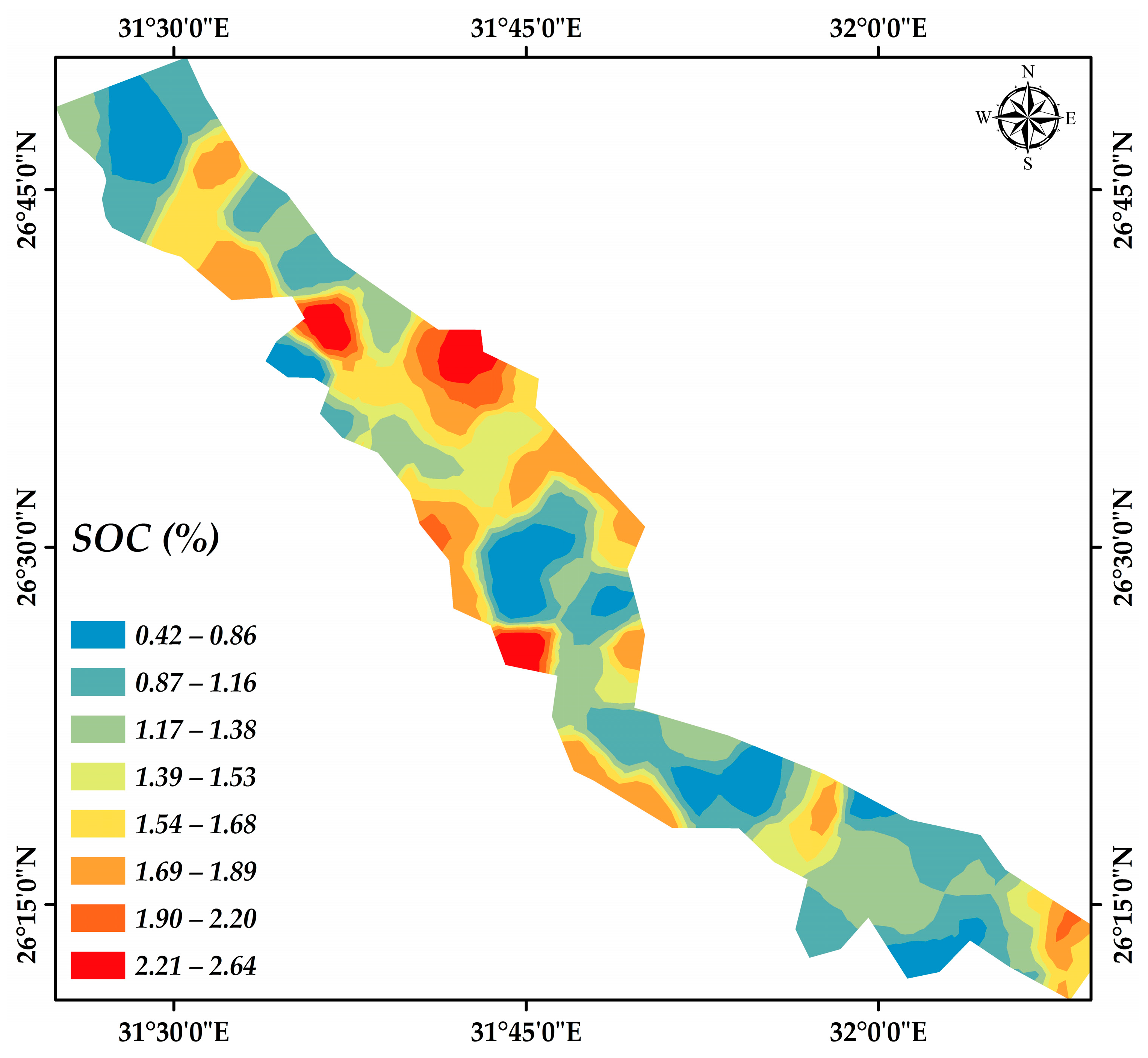
2.12. Mapping of Spatial Distribution of SOC

To show how the prediction models differ, the spatial distribution map of SOC was generated using the Ordinary Kriging (OK) interpolation method. This involved putting the predicted SOC data from each prediction model and the geographic coordinates of the soil sampling locations into Arc-GIS (ver. 10.4.1) [100]. The geostatistical assistant tool was then used to facilitate the mapping process.

3. Results and Discussions

3.1. Soil Characterization of the Study Area

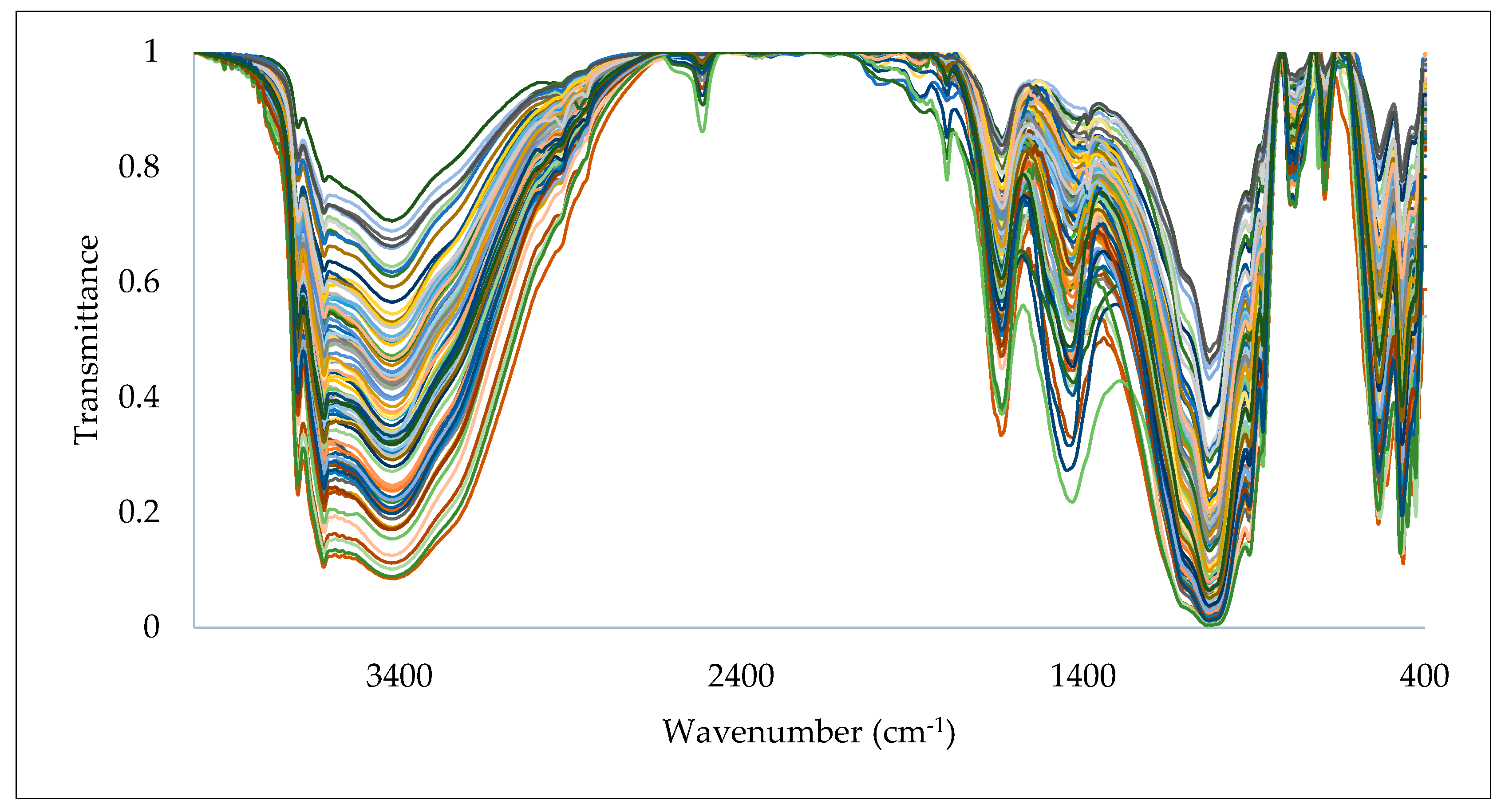
The soil samples studied are characterized in

Table 2. The characterization of the studied soil samples.

Statistical Parameter	Soil pH (1:2.5)	EC (1:2.5)	OC	CaCO3	Sand	Silt	Clay
		dS m−1            %
Mean	7.67	1.01	1.39	2.37	42.18	24.40	33.42
Standard Deviation	0.30	1.15	0.48	1.85	7.77	3.06	6.95
Minimum	7.04	0.210	0.42	0.41	10.12	15.70	18.11
Maximum	8.80	7.86	2.64	13.78	66.19	33.80	56.08

. Soil pH values ranged from 7.04 to 8.80, with a mean of 7.67, indicating a range from neutral to strongly alkaline. Most soil samples had a slightly alkaline medium environment. The soils in the study area ranged from non-saline to very saline, where EC values ranged from 0.21 to 7.86 dS m⁻¹ with an average EC value of 1.01 dS m⁻¹. The SOC ranged from 0.42 to 2.64%, with an average value of 1.39%. The calcium carbonate (CaCO₃) content of these soils ranged from 0.41 to 13.78%, with an average of 2.37%, indicating a range from non-calcareous to calcareous. Soils in the study area are classified as flat alluvial (plain) soils, with textures ranging from moderate to heavy. The sand fraction ranged from 10.12 to 66.19% with an average value of 42.18%, while the silt fraction ranged from 15.70 to 33.80% with an average value of 24.40%. The clay content of these soils ranged from 18.11 to 56.08%, with an average of 33.422%.

3.2. Soil Spectra

Soil spectral data in the range of 4000–400 cm⁻¹, obtained from the DRIFT-FTIR spectrometer, are shown in Figure 4. Comparing this spectrum with the reference spectra of known organic compounds, the content of soil organic carbon can be determined as stated in [101]. The DRIFT-FTIR spectroscopy technique can be used to identify organic carbon in soil by analyzing the detailed spectrum of the soil sample, which provides information about specific functional groups associated with organic carbon. The DRIFT-FTIR spectrum of soils is complex and includes various peaks related to different organic functional groups. For example, hydroxyl (OH) stretching vibrations, which are generally observed around 3400 cm⁻¹, are associated with the presence of organic matter in the soil, as mentioned in [102], or associated with minerals of smectite which overlap with organic matter.

Methyl C–H stretching vibrations in aliphatic compounds can be observed at specific wavenumbers, such as 2941, 2922, 2885, and 2850 cm⁻¹ [1]. Calderón et al. [58] and Shvartseva et al. [55] reported that the bands at 2925 and 2855 cm⁻¹ correspond to the asymmetric stretching vibrations of CH₃ and CH₂ groups, respectively. On the other hand, stretching vibrations of C=O bonds in carboxylic acids, esters, and ketones can be observed around 1735 cm⁻¹. It is possible that the peaks at 1640 and 1690 cm⁻¹ are the result of stretching of C=O bonds [59]. Furthermore, Huang et al. [103] and Syu and Prendergast [104] suggested that the bending observed at 1643 and 1639 cm⁻¹ is associated with the stretching of C=O and C=C bonds in aromatic compounds such as lignin and humic substances, which are generally found in soils rich in organic matter. Bands 1427 to 1433 cm⁻¹ showed carbonate minerals [62], which sometimes overlap with bands of organic material. Peaks between 1390 and 1380 cm⁻¹ indicate symmetric stretching carboxylate [19], while peaks around 1200–1300 cm⁻¹ are associated with stretching vibrations of C=O bonds in carbohydrates, cellulose, and hemicellulose.

DRIFT-FTIR spectroscopy has the ability to quantitatively analyze soil organic carbon content. It should be emphasized that the precise location and intensity of these peaks can vary depending on the composition and type of soil [105]. By calibrating a series of soil samples with known organic carbon content, a calibration curve can be established. The intensity of specific peaks in the DRIFT-FTIR spectrum associated with organic carbon can then be compared to the organic carbon content of the soil sample. This correlation allows estimation of the organic carbon content in unknown soil samples based on their DRIFT-FTIR spectra. Additionally, multivariate analysis techniques, such as partial least squares regression (PLSR) or principal component analysis (PCA), can be used to analyze DRIFT-FTIR spectra of soil samples in conjunction with their corresponding measurements of organic carbon. These techniques help identify spectral features or combinations of features that have the strongest correlation with organic carbon content.

DRIFT-FTIR spectra of soil samples can be used to generate models capable of predicting organic carbon (OC) content in new soil samples. Spectral indices provide a reliable option for estimating SOC, and specific spectral indices or ratios can be calculated from DRIFT-FTIR spectra of soil samples to estimate organic carbon content. These indices are based on the intensities or ratios of specific peaks or bands associated with organic carbon in the DRIFT-FTIR spectrum. By calibrating these indices with the measured organic carbon content, they can be used as indicators of the organic carbon content in soil samples. The DRIFT-FTIR spectrum of soil can be combined with calibration curves, multivariate analysis, or spectral indices to estimate SOC content. However, the correlation between maximum intensity and SOC content can be influenced by various factors specific to each soil type and environmental conditions. Therefore, it is crucial to consider these factors and conduct site-specific calibration and validation studies taking into account soil type and environmental conditions in order to establish accurate relationships between DRIFT-spectral characteristics. FTIR and SOC content [106]. In our study, the climatic conditions are similar in all locations of soil sampling, in addition, these soils are under the same soil type and classification with some variations in the collected soil samples’ characteristics.

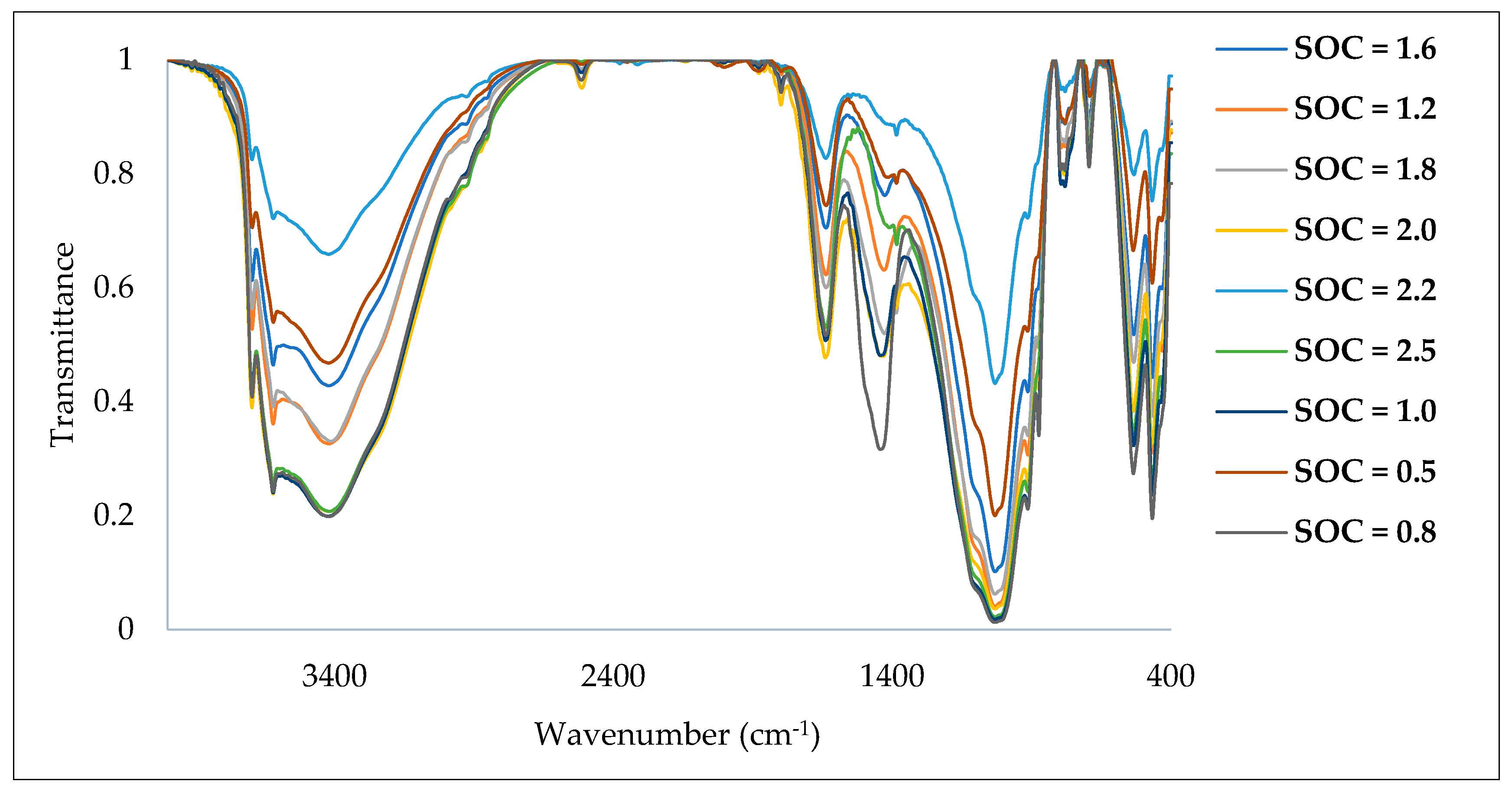
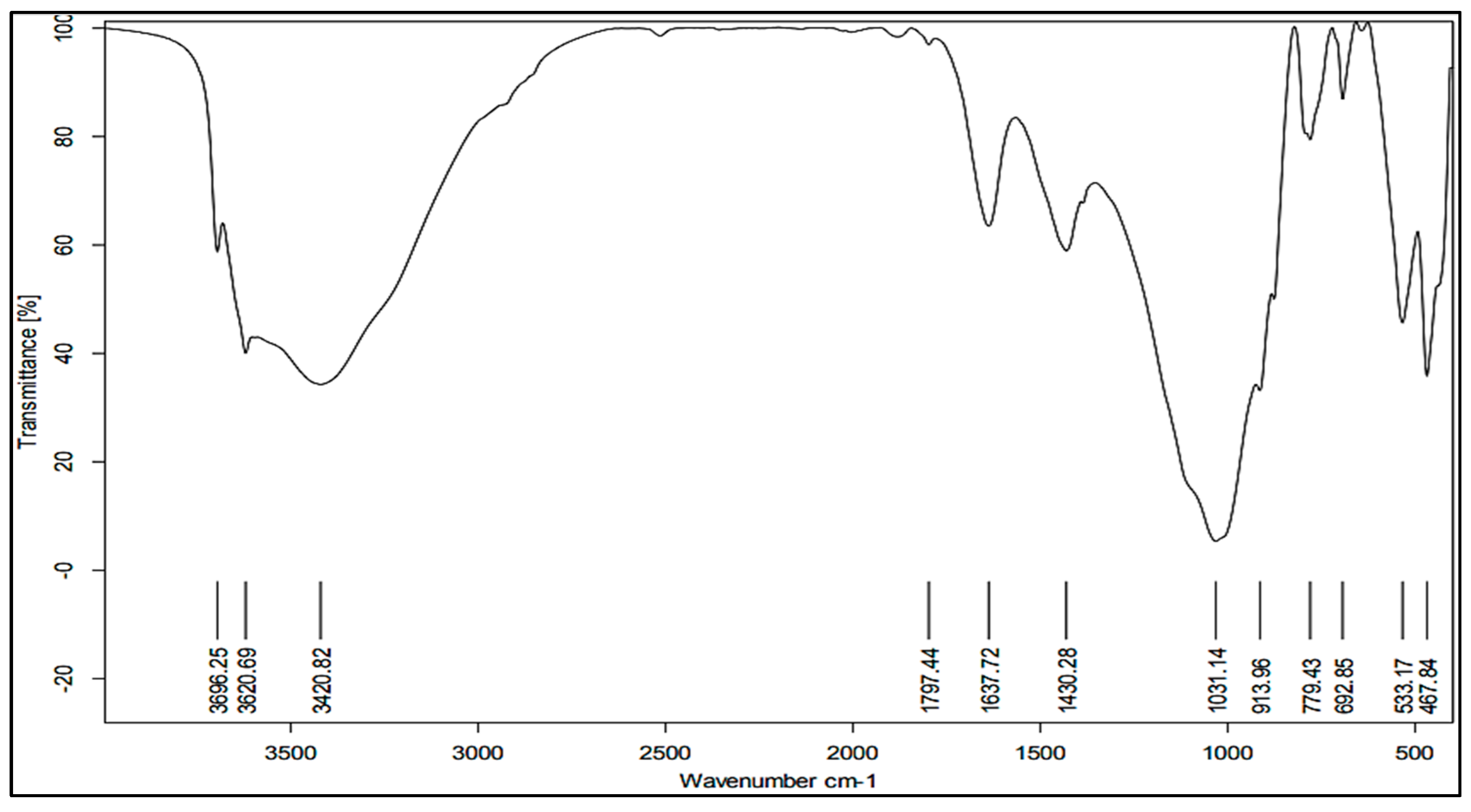
3.3. DRIFT-FTIR Spectral Behavior

From Figure 5, it is evident that there is a variation between the soil spectral signatures which is due to the variability of SOC content in the soil samples. Figure 6 shows representative DRIFT-FTIR spectral behavior as well as significant peaks (obtained from the device) for the studied soil samples. The DRIFT-FTIR spectral behavior can be concluded in three spectral regions; the first spectral region extends from 400 to 1100 cm⁻¹, while there are sharp peaks with different transmission values. The second zone varies from 1300 to 2000 cm⁻¹, which includes a few spectral peaks. The third region of the spectra extends from 3400 to 3700 cm⁻¹, while a few spectral peaks are also observed. No significant peaks were recorded in the spectral region from 2000 to 3400 cm⁻¹.

Soil spectral signatures exhibit variation, as shown in Figure 5, which can be attributed to variability in SOC content present in soil samples. Figure 6 provides a representative display of the DRIFT-FTIR spectral behavior, highlighting the significant peaks observed in the soil samples studied.

3.4. Soil Organic Carbon Prediction

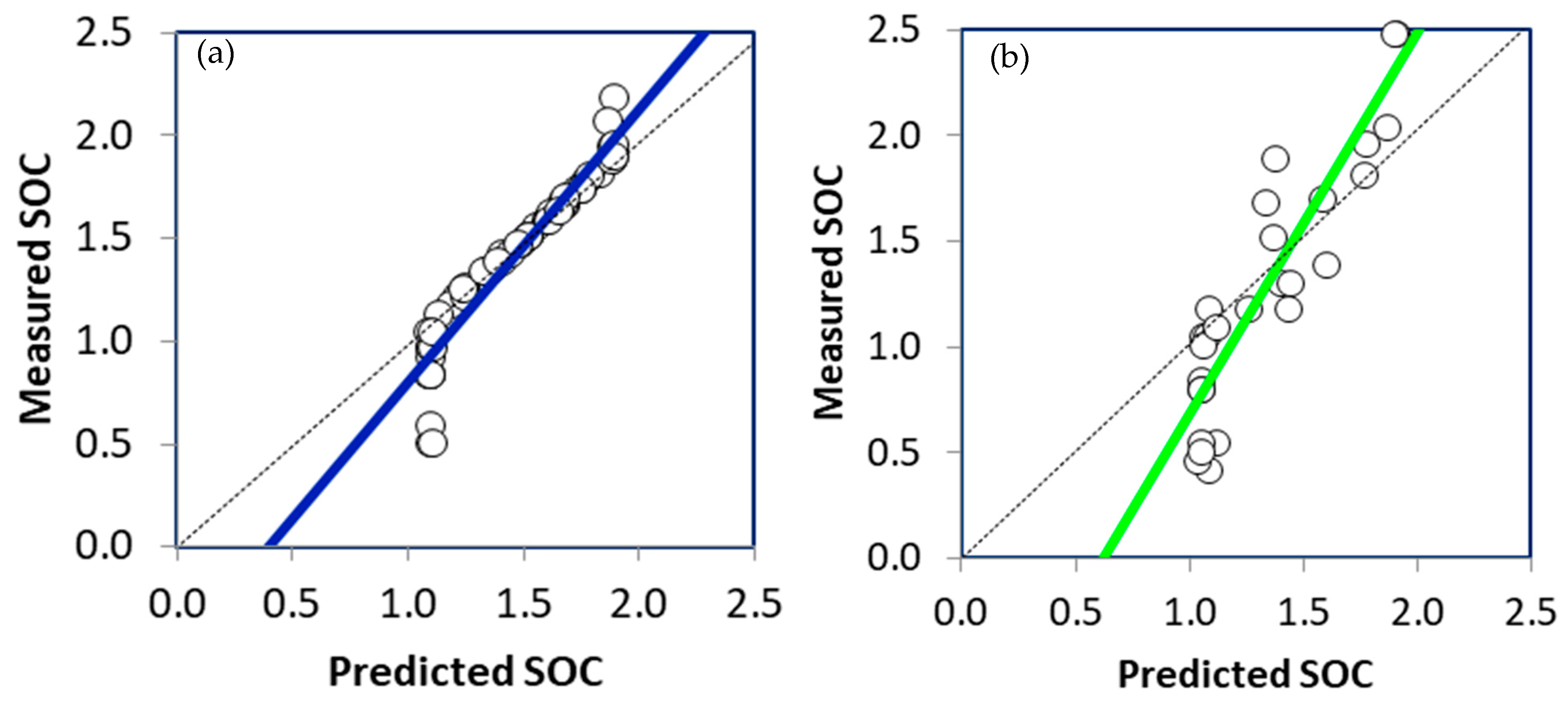
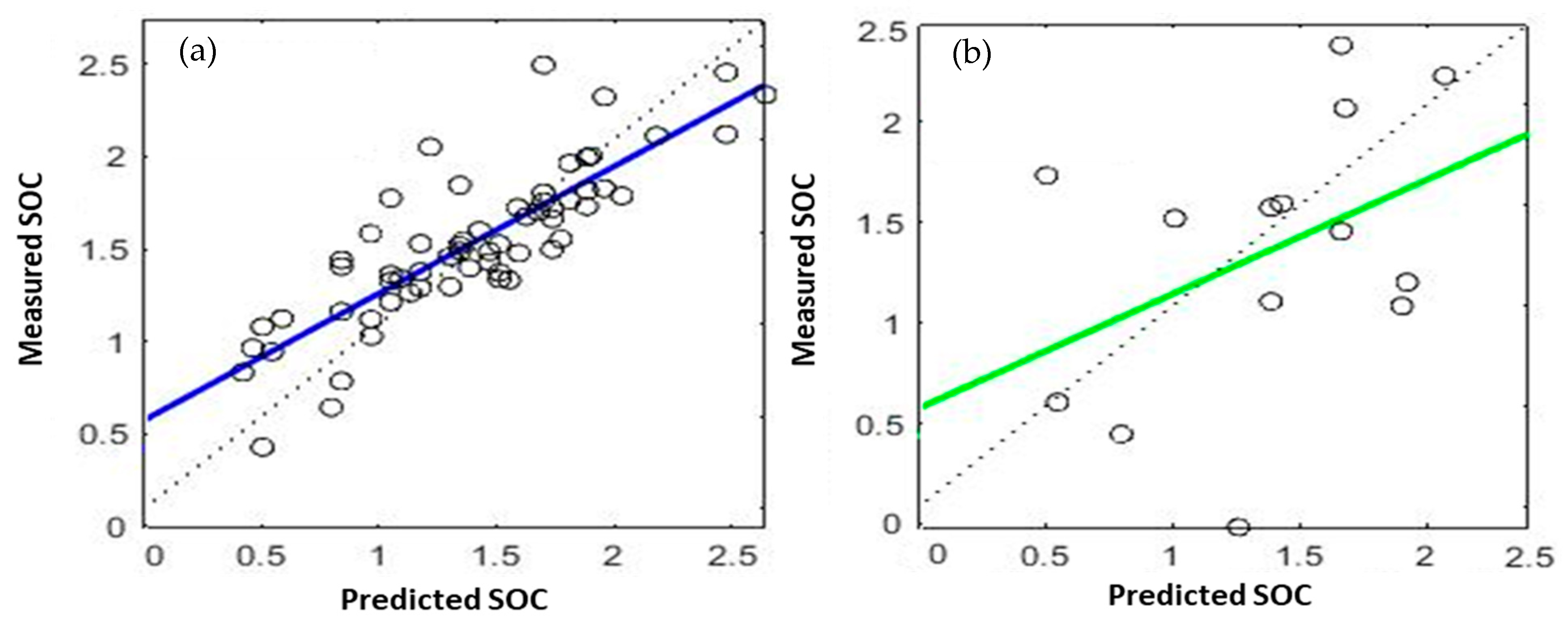
3.4.1. SOC Prediction Using PLSR

Figure 7 presents the scatter plots illustrating the comparison between measured and predicted SOC values in the calibration and validation PLSR models. The performance evaluation of the PLSR model, including R², RPD, and RMSE, is shown in

Table 3. The calibration and validation prediction models’ performance parameters.

The Prediction Model	Calibration Model (n = 60)			Regression Equation
	R2	RPD	RMSE (%)
PLSR	0.9101	1.864	0.00589	y = 1.3203x − 0.5195
ANN	0.9743	2.446	0.00433	y = 0.9800x + 0.1200
SVR	0.8018	1.571	0.00612	y = 1.0944x − 0.1346
RF	0.9633	2.236	0.00563	y = 1.4846x − 0.7143
The prediction model	Validation model (n = 26)			Regression Equation
	R2	RPD	RMSE (%)
PLSR	0.8269	1.757	0.00604	y = 1.803x − 1.1236
ANN	0.5269	1.142	0.00956	y = 0.78x + 0.19
SVR	0.2708	0.534	0.02784	y = 0.5791x + 0.4684
RF	0.1806	0.341	0.01052	y = 1.2343x − 0.5384

. The data obtained from the analysis revealed that the R² value for the PLSR calibration model was 0.9101, while the RMSE and RPD values were 0.00589%. and 1.864, respectively. In the case of the PLSR validation model, the R² value was 0.8269, with the RMSE and RPD values being 0.00604% and 1.757, respectively. Application of PLSR in conjunction with DRIFT-FTIR data allows prediction of SOC by correlating spectral measurements obtained by DRIFT-FTIR and SOC content corresponding in the soil samples. These results are consistent with previous studies conducted by [15,18,20].

Compared to other machine-learning models, PLSR exhibits higher accuracy in SOC estimation for various reasons. The main factor is handling multicollinearity, with PLSR being particularly adept at handling scenarios in which there is multicollinearity between independent variables [107]. PLSR is an appropriate method to effectively take these interactions into account [108]. By creating latent variables or components, PLSR can reduce the dimensionality of data and capture the most relevant information from the original dataset. This is particularly useful in soil science, where the number of potential predictor variables is often high relative to the number of samples available [109]. In situations where soil data sets have a relatively small number of samples compared to the number of potential predictor variables, PLSR can be robust, particularly where traditional machine-learning models may have difficulty with overfitting or instability. Soil data sets can be noisy due to inherent variability in environmental conditions and measurement errors [110]. The higher accuracy of SOC estimation can be attributed to the ability of PLSR to model and extract relevant information from datasets containing noise. In the field of soil science, where understanding the factors that impact SOC content is of significant importance, the creation of latent variables by PLSR offers valuable insights into the importance and relationships of the variables [111].

3.4.2. SOC Prediction Using ANN

Figure 8 presents the scatterplots illustrating the comparison between the measured and predicted SOC values in the calibration and validation ANN models. The performance evaluation of the ANN model is evaluated based on three factors: R², RPD, and RMSE, which are shown in Table 3. The data obtained from the analysis revealed that the R² value for the ANN calibration was 0.9743. Additionally, the RMSE and RPD values were 0.00433% and 2.446, respectively. On the other hand, the R² value for the ANN validation model was 0.5269, with corresponding RMSE and RPD values of 0.00956% and 1.142, respectively. Emadi et al. [112], predicted and mapped SOC using spectral data in some soils of Iran. They found that ANN model performed moderately which R² value of validation was 0.55.

SOC estimation using the ANN model is subject to various limitations. One of these limitations is the need for a substantial amount of data to effectively capture the complex relationships between input features and SOC [113]. Training an ANN model involves adjusting the weights of the connections between neurons based on the input data. The more data available, the more the network can learn the underlying patterns and relationships within the data. In cases where data availability is limited or the data has high variability, the ANN model may struggle to generalize accurately. Additionally, the complexity of the ANN model can lead to overfitting, especially when the training data is limited or contains noise. Overfitting can harm the generalization ability of the model, thereby affecting the accuracy of SOC estimation [113]. Moreover, the black-box nature of the ANN model can hamper its interpretability, making it difficult to understand the underlying factors that influence SOC content. In fields such as environmental sciences, interpretability plays a crucial role in obtaining valuable information about modeled processes [114]. The ANN training process can be demanding in terms of computational resources and time, especially when working with large and complex environmental datasets. Additionally, ANN requires tuning various hyperparameters, including the number of layers, neurons per layer, learning rate, and activation functions, which can be a difficult task and involve considerable trial and error. Furthermore, ANN performance in SOC estimation can be negatively affected by noisy input data, especially in environments with high variability [115].

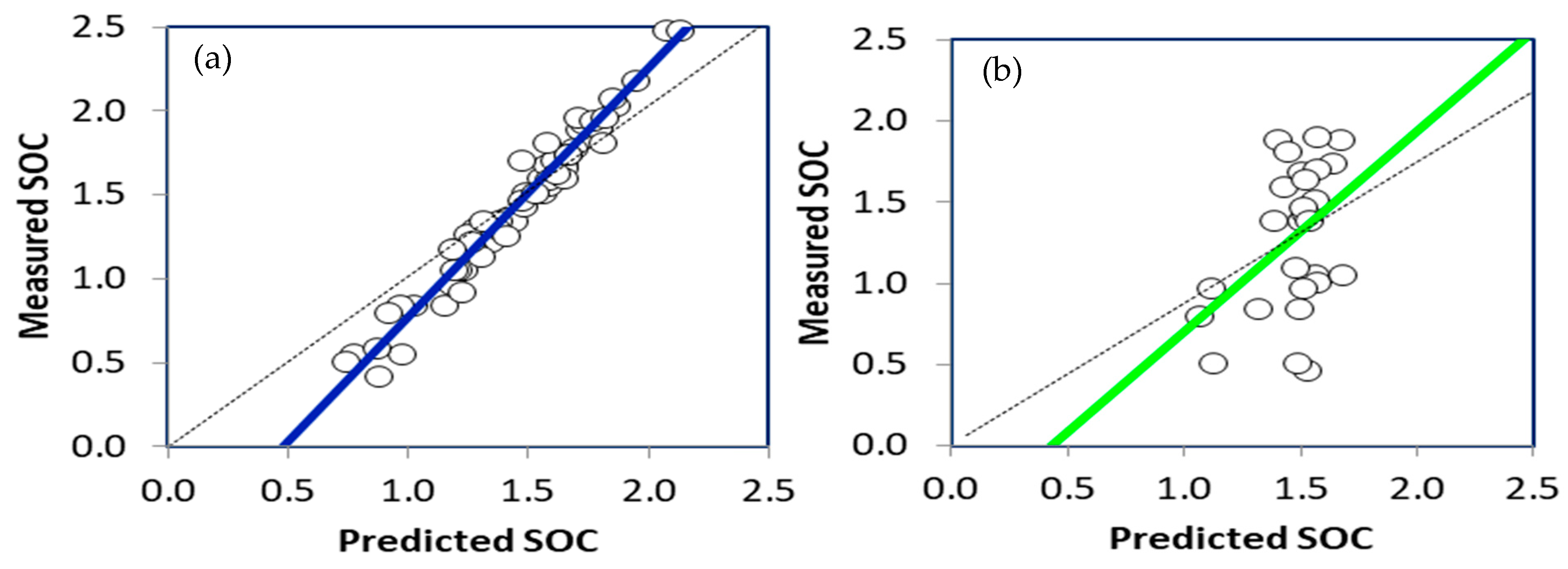
3.4.3. SOC Prediction Using SVR

The SOC values in the calibration and validation SVR models are shown as scatterplots in Figure 9, respectively. Table 3 shows the performance evaluation factors of the SVR model, including R², RPD, and RMSE. The results showed that the R² of the SVR calibration model was 0.8018, with an RMSE of 0.00612% and an RPD of 1.571. In contrast, the R² of the SVR validation model was 0.2708, with an RMSE of 0.02784% and an RPD of 0.534. Xu et al. [15] used DRIFT-FTIR data integrated with the SVR prediction model to estimate SOC, obtaining a validation R² of 0.81.

SOC estimation using the SVR prediction model is subject to several limitations. The performance of the SVR model is highly dependent on the appropriate tuning of hyperparameters, including the kernel, regularization parameter, and kernel-specific parameters. If these hyperparameters are not chosen appropriately, the performance of the SVR model might not be optimal [116]. Additionally, when dealing with large datasets, the scalability of SVR may be less effective due to its computational complexity, especially when nonlinear kernels are used [117]. Unlike other regression approaches, SVR models are not easily interpretable, which can be a limitation when trying to understand the factors influencing SOC estimation [118]. Although SVR is capable of modeling nonlinear relationships, the selection and tuning of the kernel function can have a significant impact on its performance, posing a challenge that may require domain expertise [116]. Additionally, SVR can be sensitive to noise in the input data, potentially affecting its predictive performance, particularly when the signal-to-noise ratio is low [119,120]. It is important to note that SVR does not inherently perform feature selection or handle categorical variables, making proper feature engineering crucial to ensure model effectiveness [121].

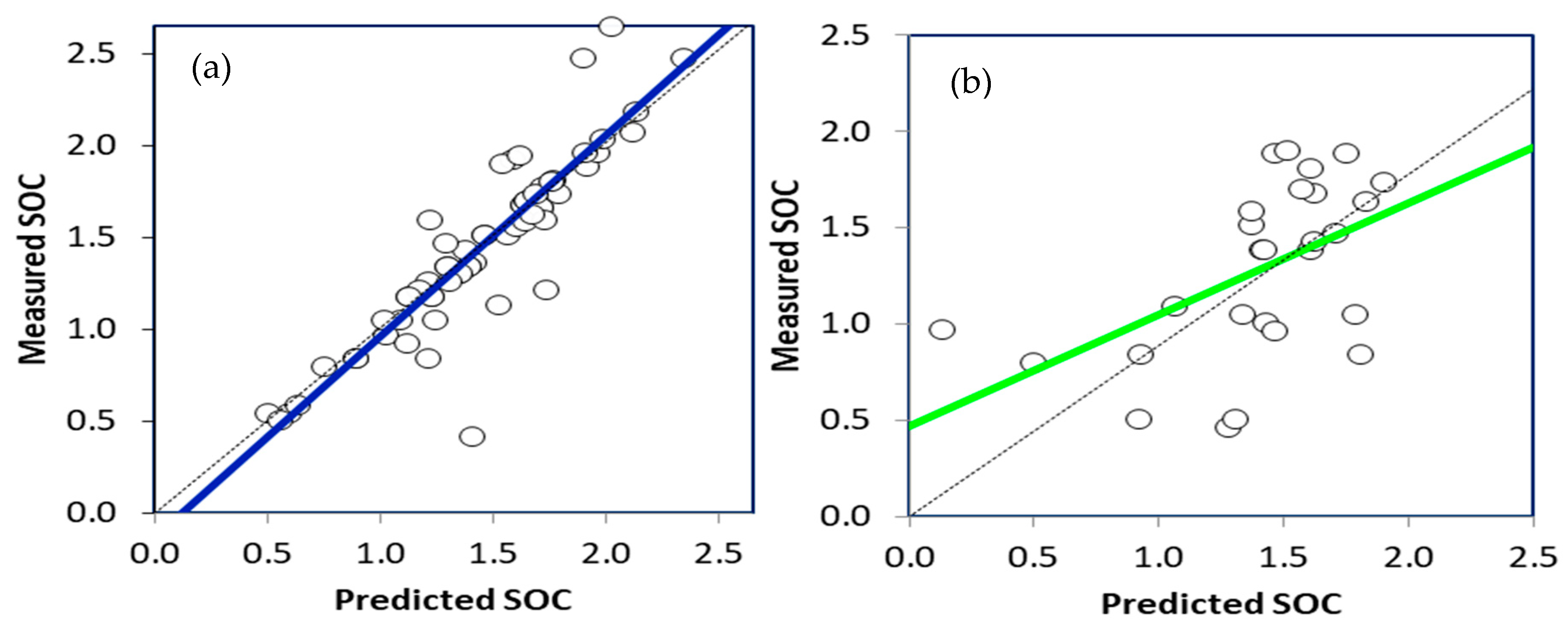
3.4.4. SOC Prediction Using RF

The scatterplots of the measured and predicted values of SOC in the calibration and validation RF models are shown in Figure 10, respectively. The data obtained from the study (Table 3) indicated that the R² of the RF calibration was 0.9633, while the RMSE and RPD were 0.00563% and 2.236, respectively. On the other hand, the R² of the RF validation model was 0.1806, while the RMSE and RPD were 0.01052% and 0.341, respectively. In a similar study, Rial et al. [122] reported an R² value of approximately 0.93 for predicting SOC using the RF model and DRIFT-FTIR soil spectral data.

There are various potential reasons why a random forest forecast model has low accuracy in SOC estimation. For any prediction model, one of the main factors is insufficient training data, which may prevent the model from accurately capturing the complexity of SOC dynamics if it was trained on a dataset limited or not representative [123]. Additionally, the selection of input features, such as soil properties, environmental factors, or geographic information, may not adequately capture SOC variability, resulting in lower predictive accuracy [124]. The model may also be overfitted to noise present in the training data, resulting in poor generalization to new data, or underfitted, failing to capture important patterns in the data. Additionally, suboptimal performance may result from inadequate tuning of model hyperparameters, such as depth or number of trees [125]. Finally, random forests, while powerful, can struggle to capture complex nonlinear relationships in SOC data if not configured appropriately [126].

3.5. Comparison between Used Machine-Learning Models

3.5.1. PLSR

The PLSR model demonstrates superior accuracy in estimating SOC because of different reasons. The main reason is that the PLSR is able to effectively manage the multicollinearity relations between the SOC laboratory or measured data and DRIFT-FTIR spectra [107,108]. The second reason is that PLSR is able to reduce the data dimensionality (caused by a high number of DRIFT-FTIR spectral data compared to the number of soil samples) and obtain the most effective information from the original data by creating several components [109]. The third reason is that the PLSR is able to be robust when a small number of samples is used. The fourth reason is that PLSR is able to extract pertinent information from datasets that contain noises (caused by inherent variability in environmental conditions and measurement errors) and after removing data outliers [110,111].

3.5.2. ANN

The ANN model has a moderate performance compared to the PLSR model due to a variety of reasons. The first reason is that a high number of soil samples is needed to find a good relation between laboratory SOC data and DRIT-FTIR spectra [113]. Training an ANN involves adjusting the weights of the connections between neurons based on the input data. The second reason that the ANN model did not perform well is because of data variability. The third reason is that the ANN model can lead to overfitting when the training data is limited or contains noise [113]. The fourth reason is the black-box nature of the ANN model in data processing is considered a big challenge for SOC data interpretation which is very important to understand the relation between SOC and DRIFT-FTIR spectra [114]. The fifth reason is that the ANN model includes a high number of neurons and layers which can involve errors [115].

3.5.3. SVR

Due to a variety of reasons, the SVR model has a poor performance for predicting SOC. The first reason is that the SVR model depends on the tuning of hyperparameters and kernel regularization whereas if there is any change in this process, the SVR predictability may not be good [116]. The second reason is the computational complexity of the SVR model when nonlinear kernels used in the presence of a small data set lead to low efficiency [117]. The third reason is that although the SVR model is capable of modeling nonlinear relations, the variability of the SOC data influences its performance negatively [118,119]. The fourth reason is that the SVR model is sensitive to noisy data and also the feature selection process which can affect the predictability of the model [120,121].

3.5.4. RF

The RF model performed poorly because of a variety of reasons. The smallness of the dataset is the first reason which can affect the performance of prediction [123]. The second reason is that the RF model doesn’t consider the spatial distribution and variability of SOC as well as the soil characteristics’ interaction which leads to poor accuracy [124]. The third reason is that the RF model may also be overfitting to noise in the used data. The fourth reason is that RF requires a large amount of data as well as inadequate tuning of hyperparameters particularly in tree depth or number of trees [125]. The fifth reason is that the RF model may not perform well with complex nonlinear relations [126].

However, the findings of this research demonstrate that the PLSR model outperforms other machine-learning models, such as ANN, RF, and SVR, in predicting SOC using DRIFT-FTIR data. PLSR is particularly adept at handling highly collinear and high-dimensional data, making it an effective tool for analyzing DRIFT-FTIR spectra. Additionally, PLSR performs well with noisy and multicollinear datasets. Furthermore, PLSR offers a straightforward approach to interpreting the relationship between the input DRIFT-FTIR data and SOC content. These benefits make PLSR a more accessible method for estimating SOC compared to traditional chemical soil analysis techniques.

3.6. Mapping of Spatial Distribution of SOC

Figure 11 illustrates the spatial arrangement of the SOC across the designated study region. The SOC distribution is represented by eight distinct colored classes, which effectively capture the range of variability in SOC levels within the area.

4. Conclusions

This study investigates the use of diffuse reflectance infrared Fourier transform spectroscopy (DRIFT-FTIR) and machine-learning models to estimate soil organic carbon (SOC) in Sohag, Egypt. The researchers collected ninety surface soil samples and estimated total organic carbon content using both the Walkley–Black method and DRIFT-FTIR spectroscopy. The spectral data were used to develop regression models using PLSR, ANN, support vector regression (SVR), and random forest (RF). The PLSR model shows the most favorable performance, yielding an R² value of 0.82 and an RMSE of 0.006%. However, the ANN, SVR, and RF models demonstrated moderate to poor performance, with R² values of 0.53, 0.27, and 0.18, respectively.

The soil samples were classified as flat (plain) alluvial soils, with texture ranging from moderate to heavy. The DRIFT-FTIR spectral behavior can be divided into three regions: 400–1100 cm⁻¹, 1300–2000 cm⁻¹, and 3400–3700 cm⁻¹. PLSR models exhibit greater accuracy in SOC estimation due to their ability to handle multicollinearity and create latent variables or components. ANN models have limitations, such as the need for a large number of soil samples, data variability, overfitting, and the black-box nature of ANN models. The performance of the SVR model depends on the appropriate tuning of hyperparameters, which can be difficult to choose and interpret. Random forest forecasting models have low accuracy in SOC estimation due to insufficient training data, selection of input features, overfitting to noise, insufficient tuning of hyperparameters, and difficulty in capturing complex nonlinear relationships in SOC data.

References

1. Thabit, F.N.; El-Shater, A.H.; Soliman, W. Role of silt and clay fractions in organic carbon and nitrogen stabilization in soils of some old fruit orchards in the Nile floodplain, Sohag Governorate, Egypt. J. Soil Sci. Plant Nutr. 2023, 23, 2525–2544. [Google Scholar] [CrossRef]
2. Mesfin, S.; Gebresamuel, G.; Haile, M.; Zenebe, A. Modelling spatial and temporal soil organic carbon dynamics under climate and land management change scenarios, northern Ethiopia. Eur. J. Soil Sci. 2021, 72, 1298–1311. [Google Scholar] [CrossRef]
3. Mostafa, S.M.; Gameh, M.A.; Abd ElWahab, M.M.; El Desoky, M.A.; Negim, O.I. Environmental negative and positive impacts of treated sewage water on the soil: A case study from Sohag Governorate, Egypt. Egypt. Sugar J. 2022, 19, 1–11. [Google Scholar] [CrossRef]
4. Ali, M.H.; Mustafa, A.R.A.; El-Sheikh, A.A. Geochemistry and spatial distribution of selected heavy metals in surface soil of Sohag, Egypt: A multivariate statistical and GIS approach. Environ. Earth Sci. 2016, 75, 1257. [Google Scholar] [CrossRef]
5. Wang, J.; Liu, T.; Zhang, J.; Yuan, H.; Acquah, G.E. Spectral variable selection for estimation of soil organic carbon content using mid--infrared spectroscopy. Eur. J. Soil Sci. 2022, 73, e13267. [Google Scholar] [CrossRef]
6. Wang, S.; Guan, K.; Zhang, C.; Lee, D.; Margenot, A.J.; Ge, Y.; Peng, J.; Zhou, W.; Zhou, Q.; Huang, Y. Using soil library hyperspectral reflectance and machine learning to predict soil organic carbon: Assessing potential of airborne and spaceborne optical soil sensing. Remote Sens. Environ. 2022, 271, 112914. [Google Scholar] [CrossRef]
7. Wiesmeier, M.; Urbanski, L.; Hobley, E.; Lang, B.; von Lützow, M.; Marin-Spiotta, E.; van Wesemael, B.; Rabot, E.; Ließ, M.; Noelia Garcia-Franco, N.; et al. Soil organic carbon storage as a key function of soils-A review of drivers and indicators at various scales. Geoderma 2019, 333, 149–162. [Google Scholar] [CrossRef]
8. Kopittke, P.M.; Dalal, R.C.; Hoeschen, C.; Li, C.; Menzies, N.W.; Mueller, C.W. Soil organic matter is stabilized by organo-mineral associations through two key processes: The role of the carbon to nitrogen ratio. Geoderma 2020, 357, 113974. [Google Scholar] [CrossRef]
9. Rocci, K.S.; Lavallee, J.M.; Stewart, C.E.; Cotrufo, M.F. Soil organic carbon response to global environmental change depends on its distribution between mineral-associated and particulate organic matter: A meta-analysis. Sci. Total Environ. 2021, 793, 148569. [Google Scholar] [CrossRef]
10. Bai, Y.; Zhang, S.; Mu, E.; Zhao, Y.; Cheng, L.; Zhu, Y.; Yuan, Y.; Wang, Y.; Ding, A. Characterizing the spatiotemporal distribution of dissolved organic matter (DOM) in the Yongding River Basin: Insights from flow regulation. J. Environ. Manag. 2023, 325, 116476. [Google Scholar] [CrossRef]
11. Pedreño, J.N.; Benslama, A.; Lucas, I.G.; Candel, M.B.A. Organic matter in farming systems in Southern Spain by LOI and Walkley-Black methods (No. EGU22-9368). In Proceedings of the 24th EGU General Assembly, Vienna, Austria, 23–27 May 2022. [Google Scholar] [CrossRef]
12. Nayak, A.K.; Rahman, M.M.; Naidu, R.; Dhal, B.; Swain, C.K.; Nayak, A.D.; Tripathi, R.; Shahid, M.; Islam, M.R.; Pathak, H. Current and emerging methodologies for estimating carbon sequestration in agricultural soils: A review. Sci. Total Environ. 2019, 665, 890–912. [Google Scholar] [CrossRef]
13. Reda, R.; Saffaj, T.; Ilham, B.; Saidi, O.; Issam, K.; Brahim, L. A comparative study between a new method and other machine learning algorithms for soil organic carbon and total nitrogen prediction using near infrared spectroscopy. Chemom. Intell. Lab. Syst. 2019, 195, 103873. [Google Scholar] [CrossRef]
14. Hong, Y.; Munnaf, M.A.; Guerrero, A.; Chen, S.; Liu, Y.; Shi, Z.; Mouazen, A.M. Fusion of visible-to-near-infrared and mid-infrared spectroscopy to estimate soil organic carbon. Soil Tillage Res. 2022, 217, 105284. [Google Scholar] [CrossRef]
15. Xu, X.; Du, C.; Ma, F.; Shen, Y.; Wu, K.; Liang, D.; Zhou, J. Detection of soil organic matter from laser-induced breakdown spectroscopy (LIBS) and mid-infrared spectroscopy (ATR-FTIR) coupled with multivariate techniques. Geoderma 2019, 355, 113905. [Google Scholar] [CrossRef]
16. Goydaragh, M.G.; Taghizadeh-Mehrjardi, R.; Jafarzadeh, A.A.; Triantafilis, J.; Lado, M. Using environmental variables and Fourier Transform Infrared Spectroscopy to predict soil organic carbon. Catena 2021, 202, 105280. [Google Scholar] [CrossRef]
17. Jović, B.; Maletić, S.; Kordić, B.; Beljin, J. DRIFT spectroscopic determination of clay and organic matter in sediment by mixed soil-sediment calibration approach. Environ. Monit. Assess. 2023, 195, 437. [Google Scholar] [CrossRef] [PubMed]
18. Xing, Z.; Du, C.; Shen, Y.; Ma, F.; Zhou, J. A method combining ATR-FTIR and Raman spectroscopy to determine soil organic matter: Improvement of prediction accuracy using competitive adaptive reweighted sampling (CARS). Comput. Electron. Agric. 2021, 191, 106549. [Google Scholar] [CrossRef]
19. Volkov, D.S.; Rogova, O.B.; Proskurnin, M.A. Organic matter and mineral composition of silicate soils: ATR- FTIR comparison study by photoacoustic, diffuse reflectance, and attenuated total reflection modalities. Agronomy 2021, 11, 1879. [Google Scholar] [CrossRef]
20. Qi, Y.P.; He, P.J.; Lan, D.Y.; Xian, H.Y.; Lü, F.; Zhang, H. Rapid determination of moisture content of multi-source solid waste using ATR-FTIR and multiple machine learning methods. Waste Manag. 2022, 153, 20–30. [Google Scholar] [CrossRef] [PubMed]
21. Davenport, R.; Bowen, B.P.; Lynch, L.M.; Kosina, S.M.; Shabtai, I.; Northen, T.R.; Lehmann, J. Decomposition decreases molecular diversity and ecosystem similarity of soil organic matter. Proc. Natl. Acad. Sci. USA 2023, 120, e2303335120. [Google Scholar] [CrossRef] [PubMed]
22. Paradelo, R.; Virto, I.; Chenu, C. Net effect of liming on soil organic carbon stocks: A review. Agric. Ecosyst. Environ. 2015, 202, 98–107. [Google Scholar] [CrossRef]
23. Hamilton, S.K.; Kurzman, A.L.; Arango, C.; Jin, L.; Robertson, G.P. Evidence for carbon sequestration by agricultural liming. Global Biogeochem. Cycles 2007, 21, GB2021. [Google Scholar] [CrossRef]
24. Huang, K.; Ma, Z.; Wang, X.; Shan, J.; Zhang, Z.; Xia, P.; Jiang, X.; Wu, X.; Huang, X. Control of soil organic carbon under karst landforms: A case study of Guizhou Province, in southwest China. Ecol. Indic. 2022, 145, 109624. [Google Scholar] [CrossRef]
25. Casby-Horton, S.; Herrero, J.; Rolong, N.A. Gypsum soils -Their morphology, classification, function, and landscapes. Adv. Agron. 2015, 130, 231–290. [Google Scholar] [CrossRef]
26. Liu, R.; Liang, B.; Zhao, H.; Zhao, Y. Impacts of various amendments on the microbial communities and soil organic carbon of coastal saline–alkali soil in the Yellow River Delta. Front. Microbiol. 2023, 14, 1239855. [Google Scholar] [CrossRef] [PubMed]
27. Gholizadeh, A.; Carmon, N.; Klement, A.; Ben-Dor, E.; Borůvka, L. Agricultural soil spectral response and properties assessment: Effects of measurement protocol and data mining technique. Remote Sens. 2017, 9, 1078. [Google Scholar] [CrossRef]
28. Segneanu, A.E.; Gozescu, I.; Dabici, A.; Sfirloaga, P.; Szabadai, Z. Organic Compounds FT-IR Spectroscopy; InTech: Rijeka, Croatia, 2012; p. 145. [Google Scholar]
29. Guerrero-Pérez, M.O.; Patience, G.S. Experimental methods in chemical engineering: Fourier transform infrared spectroscopy-ATR-FTIR. Can. J. Chem. Eng. 2020, 98, 25–33. [Google Scholar] [CrossRef]
30. Pucetaite, M.; Arellano, C.; Ohlsson, P.; Persson, P.; Hammer, E. Macro ATR- FTIR imaging for better understanding of organic matter dynamics in soil. In Proceedings of the EGU General Assembly Conference 2021, online, 19–30 April 2021; Abstracts. pp. EGU21–14325. [Google Scholar] [CrossRef]
31. Okunev, R.; Smirnova, E.; Giniyatullin, K.; Sahabiev, I.; Gordeeva, K. Application of ATR-FTIR spectrometry for express prediction of the organic matter properties of arable leached chernozem. Int. Multidiscip. Sci. GeoConference Surv. Geol. Min. Ecol. Manag. SGEM 2020, 3, 381–386. Available online: https://repository.kpfu.ru/eng/?p_id=249201&p_lang=2 (accessed on 26 October 2023).
32. Bellon-Maurel, V.; Fernandez-Ahumada, E.; Palagos, B.; Roger, J.M.; McBratney, A. Critical review of chemometric indicators commonly used for assessing the quality of the prediction of soil attributes by NIR spectroscopy. TrAC Trends Anal. Chem. 2010, 29, 1073–1081. [Google Scholar] [CrossRef]
33. Hong, Y.; Chen, S.; Zhang, Y.; Chen, Y.; Yu, L.; Liu, Y.; Liu, Y.; Cheng, H.; Liu, Y. Rapid identification of soil organic matter level via visible and near-infrared spectroscopy: Effects of two-dimensional correlation coefficient and extreme learning machine. Sci. Total Environ. 2018, 644, 1232–1243. [Google Scholar] [CrossRef]
34. Xu, X.; Du, C.; Ma, F.; Qiu, Z.; Zhou, J. A framework for high-resolution mapping of soil organic matter (SOM) by the integration of fourier mid-infrared attenuation total reflectance spectroscopy (ATR-FTIR), sentinel-2 images, and DEM derivatives. Remote Sens. 2023, 15, 1072. [Google Scholar] [CrossRef]
35. Veum, K.S.; Goyne, K.W.; Kremer, R.J.; Miles, R.J.; Sudduth, K.A. Biological indicators of soil quality and soil organic matter characteristics in an agricultural management continuum. Biogeochemistry 2014, 117, 81–99. [Google Scholar] [CrossRef]
36. Calderón, F.J.; Culman, S.; Six, J.; Franzluebbers, A.J.; Schipanski, M.; Beniston, J.; Grandy, S.; Kong, A.Y. Quantification of soil permanganate oxidizable C (POXC) using infrared spectroscopy. Soil Sci. Soc. Am. J. 2017, 81, 277–288. [Google Scholar] [CrossRef]
37. Margenot, A.; O'Neill, T.; Sommer, R.; Akella, V. Predicting soil permanganate oxidizable carbon (POXC) by coupling DRIFT spectroscopy and artificial neural networks (ANN). Comput. Electron. Agric. 2020, 168, 105098. [Google Scholar] [CrossRef]
38. Barstow, T.J. Understanding near infrared spectroscopy and its application to skeletal muscle research. J. Appl. Physiol. 2019, 126, 1360–1376. [Google Scholar] [CrossRef] [PubMed]
39. Smith, E.; Dent, G. Modern Raman Spectroscopy: A Practical Approach; John Wiley & Sons: Chichester, UK, 2019; p. 210. [Google Scholar] [CrossRef]
40. Dangal, S.R.; Sanderman, J.; Wills, S.; Ramirez-Lopez, L. Accurate and precise prediction of soil properties from a large mid-infrared spectral library. Soil Syst. 2019, 3, 11. [Google Scholar] [CrossRef]
41. Zhu, Z.; Minasny, B.; Field, D.J.; An, S. Using mid-infrared diffuse reflectance spectroscopy to investigate the dynamics of soil aggregate formation in a clay soil. Catena 2023, 231, 107366. [Google Scholar] [CrossRef]
42. Baes, A.U.; Bloom, P.R. Diffuse reflectance and transmission Fourier transform infrared (DRIFT) spectroscopy of humic and fulvic acids. Soil Sci. Soc. Am. J. 1989, 53, 695–700. [Google Scholar] [CrossRef]
43. IUSS Working Group WRB. World Reference Base for Soil Resources. In International Soil Classification System for Naming Soils and Creating Legends for Soil Maps, 4th ed.; International Union of Soil Sciences (IUSS): Vienna, Austria, 2022. [Google Scholar]
44. Abdelhafez, S. Agriculture and soil survey in Egypt. In Soil Resources of Southern and Eastern Mediterranean Countries; Zdruli, P., Steduto, P., Lacirignola, C., Montanarella, L., Eds.; Options Méditerranéennes: Série B. Etudes et Recherches; n. 34; CIHEAM: Bari, Italy, 2001; pp. 111–125. [Google Scholar]
45. Aslan-Sungur, G.; Evrendilek, F.; Karakaya, N.; Gungor, K.; Kilic, S. Integrating ATR- FTIR and data-driven models to predict total soil carbon and nitrogen towards sustainable watershed management. Res. J. Chem. Environ. 2013, 17, 5–11. [Google Scholar]
46. Tiruneh, G.A.; Meshesha, D.T.; Adgo, E.; Tsunekawa, A.; Haregeweyn, N.; Fenta, A.A.; Alemayehu, T.Y.; Ayana, G.; Reichert, J.M.; Tilahun, K. Geospatial modeling and mapping of soil organic carbon and texture from spectroradiometric data in Nile basin. Remote Sens. Appl. Soc. Environ. 2023, 29, 100879. [Google Scholar] [CrossRef]
47. Jackson, M.L. Soil Chemical Analysis; Prentice Hall, Inc.: Englewood Cliffs, NJ, USA, 1973; p. 498. [Google Scholar] [CrossRef]
48. Jackson, M.L. Soil Chemical Analysis—Advanced Course; UW-Madison Libraries Parallel Press: Madison, WI, USA, 1969. [Google Scholar]
49. Nelson, D.W.; Sommers, L.E. Total Carbon, Organic Carbon, and Organic Matter. In Methods of Soil Analysis, Part 3 Chemical Methods, 5; John Wiley & Sons: Hoboken, NJ, USA, 1996; pp. 961–1010. [Google Scholar]
50. Margenot, A.J.; Calderón, F.J.; Parikh, S.J. Limitations and potential of spectral subtractions in Fourier-transform infrared spectroscopy of soil samples. Soil Sci. Soc. Am. J. 2016, 80, 10–26. [Google Scholar] [CrossRef]
51. Janik, L.J.; Skjemstad, J.O. Characterization and analysis of soils using midinfrared partial least-squares. 2. Correlations with some laboratory data. Aust. J. Soil Res. 1995, 33, 637–650. [Google Scholar] [CrossRef]
52. Jozanikohan, G.; Abarghooei, M.N. The Fourier transform infrared spectroscopy (FTIR) analysis for the clay mineralogy studies in a clastic reservoir. J. Pet. Explor. Prod. Technol. 2022, 12, 2093–2106. [Google Scholar] [CrossRef]
53. Sharma, V.; Chauhan, R.; Kumar, R. Spectral characteristics of organic soil matter: A comprehensive review. Microchem. J. 2021, 171, 106836. [Google Scholar] [CrossRef]
54. Ellerbrock, R.H.; Höhn, A.; Gerke, H. Characterization of soil organic matter from a sandy soil in relation to management practice using FT-IR spectroscopy. Plant Soil 1999, 213, 55–61. [Google Scholar] [CrossRef]
55. Shvartseva, O.; Skripkina, T.; Gaskova, O.; Podgorbunskikh, E. Modification of natural peat for removal of copper ions from aqueous solutions. Water 2022, 14, 2114. [Google Scholar] [CrossRef]
56. Reddy, S.B.; Nagaraja, M.S.; Kadalli, G.G.; Champa, B.V. Fourier transform infrared (FTIR) spectroscopy of soil humic and fulvic acids extracted from paddy land use system. Int. J. Curr. Microbiol. Appl. Sci. 2018, 7, 834–837. [Google Scholar] [CrossRef]
57. Cepus, V.; Borth, M.; Seitz, M. IR spectroscopic characterization of lignite as a tool to predict the product range of catalytic decomposition. Int. J. Clean Coal Energy 2016, 5, 13. [Google Scholar] [CrossRef]
58. Calderón, F.; Haddix, M.; Conant, R.; Magrini-Bair, K.; Paul, E. Diffuse-reflectance Fourier-transform mid-infrared spectroscopy as a method of characterizing changes in soil organic matter. Soil Sci. Soc. Am. J. 2013, 77, 1591–1600. [Google Scholar] [CrossRef]
59. Sarkhot, D.V.; Comerford, N.; Jokela, E.J.; Reeves, J.B.; Harris, W.G. Aggregation and aggregate carbon in a forested southeastern coastal plain spodosol. Soil Sci. Soc. Am. J. 2007, 71, 1779–1787. [Google Scholar] [CrossRef]
60. Song, Y.; Feng, W.; Li, N.; Li, Y.; Zhi, K.; Teng, Y.; He, R.; Zhou, H.; Liu, Q. Effects of demineralization on the structure and combustion properties of Shengli lignite. Fuel 2016, 183, 659–667. [Google Scholar] [CrossRef]
61. Lima, D.L.; Santos, S.M.; Scherer, H.W.; Schneider, R.J.; Duarte, A.C.; Santos, E.B.; Esteves, V.I. Effects of organic and inorganic amendments on soil organic matter properties. Geoderma 2009, 150, 38–45. [Google Scholar] [CrossRef]
62. Kim, Y.; Caumon, M.C.; Barres, O.; Sall, A.; Cauzid, J. Identification and composition of carbonate minerals of the calcite structure by Raman and infrared spectroscopies using portable devices. Spectro-Chim. Acta Part A. Mol. Biomol. Spectrosc. 2021, 261, 119980. [Google Scholar] [CrossRef] [PubMed]
63. Müller, C.M.; Pejcic, B.; Esteban, L.; Piane, C.D.; Raven, M.; Mizaikoff, B. Infrared attenuated total reflectance spectroscopy: An innovative strategy for analyzing mineral components in energy relevant systems. Sci. Rep. 2014, 4, 6764. [Google Scholar] [CrossRef] [PubMed]
64. Zaccone, C.; Cocozza, C.; D’Orazio, V.; Plaza, C.; Cheburkin, A.; Miano, T.M. Influence of extractant on quality and trace elements content of peat humic acids. Talanta 2007, 73, 820–830. [Google Scholar] [CrossRef] [PubMed]
65. Janik, L.J.; Merry, R.H.; Forrester, S.; Lanyon, D.; Rawson, A. Rapid prediction of soil water retention using mid infrared spectroscopy. Soil Sci. Soc. Am. J. 2007, 71, 507–514. [Google Scholar] [CrossRef]
66. Janik, L.J.; Skjemstad, J.; Shepherd, K.; Spouncer, L. The prediction of soil carbon fractions using mid-infrared-partial least square analysis. Aust. J. Soil Res. 2007, 45, 73–81. [Google Scholar] [CrossRef]
67. Zaccone, C.; Miano, T.M.; Shotyk, W. Qualitative comparison between raw peat and related humic acids in an ombrotrophic bog profile. Org. Geochem. 2007, 38, 151–160. [Google Scholar] [CrossRef]
68. Madejova, J. ATR-FTIR techniques in clay mineral studies. Vib. Spectrosc. 2003, 31, 1–10. [Google Scholar] [CrossRef]
69. Nayak, P.S.; Singh, B. Instrumental characterization of clay by XRF, XRD and ATR-FTIR. Bull. Mater. Sci. 2007, 30, 235–238. [Google Scholar] [CrossRef]
70. Rossel, R.V.; Behrens, T. Using data mining to model and interpret soil diffuse reflectance spectra. Geoderma 2010, 158, 46–54. [Google Scholar] [CrossRef]
71. Abou-El-Sherbini, K.S.; Elzahany, E.A.; Wahba, M.A.; Drweesh, S.A.; Youssef, N.S. Evaluation of some intercalation methods of dimethylsulphoxide onto HCl-treated and untreated Egyptian kaolinite. Appl. Clay Sci. 2017, 137, 33–42. [Google Scholar] [CrossRef]
72. Box, G.E.; Cox, D.R. An analysis of transformations. J. R. Stat. Soc. Ser. B Stat. Methodol. 1964, 26, 211–243. [Google Scholar] [CrossRef]
73. R Core Team. R: A Language and Environment for Statistical Computing; R Foundation for Statistical Computing: Vienna, Austria, 2018; Available online: https://www.R-project.org/ (accessed on 3 December 2023).
74. Knief, U.; Forstmeier, W. Violating the normality assumption may be the lesser of two evils. Behav. Res. Methods 2021, 53, 2576–2590. [Google Scholar] [CrossRef]
75. Guo, L.; Fu, P.; Shi, T.; Chen, Y.; Zeng, C.; Zhang, H.; Wang, S. Exploring influence factors in mapping soil organic carbon on low-relief agricultural lands using time series of remote sensing data. Soil Tillage Res. 2021, 210, 104982. [Google Scholar] [CrossRef]
76. Xie, S.; Ding, F.; Chen, S.; Wang, X.; Li, Y.; Ma, K. Prediction of soil organic matter content based on characteristic band selection method. Spectrochim. Acta Part A Mol. Biomol. Spectrosc. 2022, 273, 120949. [Google Scholar] [CrossRef]
77. Hong, Y.; Chen, S.; Hu, B.; Wang, N.; Xue, J.; Zhuo, Z.; Yang, Y.; Chen, Y.; Peng, J.; Liu, Y.; et al. Spectral fusion modeling for soil organic carbon by a parallel input-convolutional neural network. Geoderma 2023, 437, 116584. [Google Scholar] [CrossRef]
78. Martens, H.; Næs, T. Multivariate Calibration; John Wiley and Sons: Chichester, UK, 1989; p. 419. [Google Scholar] [CrossRef]
79. Efron, B.; Tibshirani, R.J. An Introduction to the Bootstrap; CRC Press: New York, NY, USA, 1994; p. 456. [Google Scholar] [CrossRef]
80. Zhang, Z.; Ding, J.; Zhu, C.; Wang, J. Combination of efficient signal pre-processing and optimal band combination algorithm to predict soil organic matter through visible and near-infrared spectra. Spectrochim. Acta Part A Mol. Biomol. Spectrosc. 2020, 240, 118553. [Google Scholar] [CrossRef]
81. Paul, S.S.; Coops, N.C.; Johnson, M.S.; Krzic, M.; Chandna, A.; Smukler, S.M. Mapping soil organic carbon and clay using remote sensing to predict soil workability for enhanced climate change adaptation. Geoderma 2020, 363, 114177. [Google Scholar] [CrossRef]
82. Prashanth, D.S.; Mehta, R.V.K.; Sharma, N. Classification of handwritten Devanagari number–an analysis of pattern recognition tool using neural network and CNN. Procedia Comput. Sci. 2020, 167, 2445–2457. [Google Scholar] [CrossRef]
83. Xu, L.; Mei, X.; Chang, J.; Wu, G.; Jin, Q.; Wang, X. Rapid assessment of quality changes in french fries during deep-frying based on ATR-FTIR spectroscopy combined with artificial neural network. J. Oleo Sci. 2021, 70, 1373–1380. [Google Scholar] [CrossRef] [PubMed]
84. Boger, Z.; Guterman, H. Knowledge extraction from artificial neural network models. In 1997 IEEE International Conference on Systems, Man, and Cybernetics. Comput. Cybern. Simul. 1997, 4, 3030–3035. [Google Scholar] [CrossRef]
85. Gan, F.; Wu, K.; Ma, F.; Wei, C.; Du, C. In-situ monitoring of nitrate in industrial wastewater using Fourier transform infrared attenuated total reflectance spectroscopy (ATR-FTIR) coupled with chemometrics methods. Heliyon 2022, 8, e12423. [Google Scholar] [CrossRef] [PubMed]
86. Enders, A.; North, N.; Clark, J.; Allen, H. Saccharide concentration prediction from proxy-sea surface microlayer samples analyzed via ATR-ATR-FTIR spectroscopy and quantitative machine learning. Anal. Chem. 2023. preprint. [Google Scholar] [CrossRef]
87. Stenberg, B. Effects of soil sample pretreatments and standardized rewetting as interacted with sand classes on Vis-NIR predictions of clay and soil organic carbon. Geoderma 2010, 158, 15–22. [Google Scholar] [CrossRef]
88. Vapnik, V. The Nature of Statistical Learning Theory; Springer: New York, NY, USA, 2000; p. 314. [Google Scholar] [CrossRef]
89. De Brabanter, K.; De Brabanter, J.; Gijbels, I.; De Moor, B. Derivative estimation with local polynomial fitting. J. Mach. Learn. Res. 2013, 14, 281–301. [Google Scholar]
90. Stone, M. Cross-validation and multinomial prediction. Biometrika 1974, 61, 509–515. [Google Scholar] [CrossRef]
91. Suykens, J.A.; De Brabanter, J.; Lukas, L.; Vandewalle, J. Weighted least squares support vector machines: Robustness and sparse approximation. Neurocomputing 2002, 48, 85–105. [Google Scholar] [CrossRef]
92. Mouazen, A.M.; Kuang, B.; De Baerdemaeker, J.; Ramon, H. Comparison among principal component, partial least squares and back propagation neural network analyses for accuracy of measurement of selected soil properties with visible and near infrared spectroscopy. Geoderma 2010, 158, 23–31. [Google Scholar] [CrossRef]
93. Nguyen, J.M.; Jézéquel, P.; Gillois, P.; Silva, L.; Ben Azzouz, F.; Lambert-Lacroix, S.; Juin, P.; Campone, M.; Gaultier, A.; Moreau-Gaudry, A.; et al. Random forest of perfect trees: Concept, performance, applications and perspectives. Bioinformatics 2021, 37, 2165–2174. [Google Scholar] [CrossRef] [PubMed]
94. Parmar, A.; Katariya, R.; Patel, V. A Review on Random Forest: An Ensemble Classifier. In International Conference on Intelligent Data Communication Technologies and Internet of Things (ICICI) 2018; Hemanth, J., Fernando, X., Lafata, P., Baig, Z., Eds.; Lecture Notes on Data Engineering and Communications Technologies; Springer: Cham, Switzerland, 2019; Volume 26. [Google Scholar] [CrossRef]
95. Hong, Y.; Chen, S.; Chen, Y.; Linderman, M.; Mouazen, A.M.; Liu, Y.; Guo, L.; Yu, L.; Liu, Y.; Cheng, H.; et al. Comparing laboratory and airborne hyperspectral data for the estimation and mapping of topsoil organic carbon: Feature selection coupled with random forest. Soil Tillage Res. 2020, 199, 104589. [Google Scholar] [CrossRef]
96. Liu, J.; Dong, Z.; Xia, J.; Wang, H.; Meng, T.; Zhang, R.; Han, J.; Wang, N.; Xie, J. Estimation of soil organic matter content based on CARS algorithm coupled with random forest. Spectrochim. Acta Part A Mol. Biomol. Spectrosc. 2021, 258, 119823. [Google Scholar] [CrossRef]
97. Ghosh, S.A.K.; Hati, K.M.; Sinha, N.K.; Mridha, N.; Sahu, B. Regional soil organic carbon prediction models based on a multivariate analysis of the Mid-infrared hyperspectral data in the middle Indo-Gangetic plains of India. Infrared Phys. Technol. 2022, 127, 104372. [Google Scholar] [CrossRef]
98. Breiman, L. Random forests. Mach. Learn. 2001, 45, 5–32. Available online: https://link.springer.com/content/pdf/10.1023/A:1010933404324.pdf (accessed on 29 January 2024). [CrossRef]
99. Quinlan, J.R. Combining instance-based and model-based learning. In Proceedings of the Tenth International Conference on Machine Learning, University of Massachussetts, Amherst, MA, USA, 27–29 June 1993; pp. 236–243. [Google Scholar] [CrossRef]
100. ESRI. Arc Map version 10.4.1 User Manual; ESRI: Redlands, CA, USA, 2016. [Google Scholar]
101. Solomon, D.; Lehmann, J.; Kinyangi, J.; Liang, B.; Schäfer, T. Carbon K--edge NEXAFS and ATR-FTIR spectroscopic investigation of organic carbon speciation in soils. Soil Sci. Soc. Am. J. 2005, 69, 107–119. [Google Scholar] [CrossRef]
102. Zhang, X.; Li, Y.; Ye, J.; Chen, Z.; Ren, D.; Zhang, S. The spectral characteristics and cadmium complexation of soil dissolved organic matter in a wide range of forest lands. Environ. Pollut. 2022, 299, 118834. [Google Scholar] [CrossRef] [PubMed]
103. Huang, M.; Li, Z.; Huang, B.; Luo, N.; Zhang, Q.; Zhai, X.; Zeng, G. Investigating binding characteristics of cadmium and copper to DOM derived from compost and rice straw using EEM-PARAFAC combined with two-dimensional ATR-FTIR correlation analyses. J. Hazard. Mater. 2018, 344, 539–548. [Google Scholar] [CrossRef] [PubMed]
104. Syu, V.; Prendergast, F.G. Water (H2O and D2O) molar absorptivity in the 1000–4000 cm-1 range and quantitative infrared spectroscopy of aqueous solutions. Anal. Biochem. 1997, 248, 234–245. [Google Scholar] [CrossRef]
105. Krivoshein, P.K.; Volkov, D.S.; Rogova, O.B.; Proskurnin, M.A. ATR-FTIR Photoacoustic and ATR Spectroscopies of Soils with Aggregate Size Fractionation by Dry Sieving. ACS Omega 2022, 7, 2177–2197. [Google Scholar] [CrossRef]
106. Haddaway, N.R.; Hedlund, K.; Jackson, L.E.; Kätterer, T.; Lugato, E.; Thomsen, I.K.; Jørgensen, H.B.; Isberg, P.E. How does tillage intensity affect soil organic carbon? A systematic review. Environ. Evid. 2017, 6, 30. [Google Scholar] [CrossRef]
107. Guven, G.; Samkar, H. Examination of dimension reduction performances of PLSR and PCR techniques in data with multicollinearity. Iran. J. Sci. Technol. Trans. A Sci. 2019, 43, 969–978. [Google Scholar] [CrossRef]
108. Luo, Z.; Feng, W.; Luo, Y.; Baldock, J.; Wang, E. Soil organic carbon dynamics jointly controlled by climate, carbon inputs, soil properties and soil carbon fractions. Glob. Change Biol. 2017, 23, 4430–4439. [Google Scholar] [CrossRef]
109. Hu, J.; Fang, J.; Du, Y.; Liu, Z.; Ji, P. Application of PLS algorithm in discriminant analysis in multidimensional data mining. J. Supercomput. 2019, 75, 6004–6020. [Google Scholar] [CrossRef]
110. Tsimpouris, E.; Tsakiridis, N.L.; Theocharis, J.B. Using autoencoders to compress soil VNIR–SWIR spectra for more robust prediction of soil properties. Geoderma 2021, 393, 114967. [Google Scholar] [CrossRef]
111. Das, B.; Chakraborty, D.; Singh, V.K.; Das, D.; Sahoo, R.N.; Aggarwal, P.; Murgaokar, D.; Mondal, B.P. Partial least square regression-based machine learning models for soil organic carbon prediction using visible–near infrared spectroscopy. Geoderma Reg. 2023, 33, e00628. [Google Scholar] [CrossRef]
112. Emadi, M.; Taghizadeh-Mehrjardi, R.; Cherati, A.; Danesh, M.; Mosavi, A.; Scholten, T. Predicting and mapping of soil organic carbon using machine learning algorithms in Northern Iran. Remote Sens. 2020, 12, 2234. [Google Scholar] [CrossRef]
113. El-Sefy, M.; Yosri, A.; El-Dakhakhni, W.; Nagasaki, S.; Wiebe, L. Artificial neural network for predicting nuclear power plant dynamic behaviors. Nucl. Eng. Technol. 2021, 53, 3275–3285. [Google Scholar] [CrossRef]
114. Bodini, M.; Rivolta, M.W.; Sassi, R. Opening the black box: Interpretability of machine learning algorithms in electrocardiography. Philos. Trans. R. Soc. A 2021, 379, 20200253. [Google Scholar] [CrossRef] [PubMed]
115. Li, J.; Liu, Y.; Yin, C.; Ren, X.; Su, Y. Fast imaging of time-domain airborne EM data using deep learning technology. Geophysics 2020, 85, E163–E170. [Google Scholar] [CrossRef]
116. Saha, P.; Debnath, P.; Thomas, P. Prediction of fresh and hardened properties of self-compacting concrete using support vector regression approach. Neural Comput. Appl. 2020, 32, 7995–8010. Available online: https://link.springer.com/article/10.1007/s00521-019-04267-w (accessed on 25 January 2024). [CrossRef]
117. Wu, J.; Wang, Y.G.; Tian, Y.C.; Burrage, K.; Cao, T. Support vector regression with asymmetric loss for optimal electric load forecasting. Energy 2021, 223, 119969. [Google Scholar] [CrossRef]
118. Chaibi, M.; Benghoulam, E.M.; Tarik, L.; Berrada, M.; Hmaidi, A.E. An interpretable machine learning model for daily global solar radiation prediction. Energies 2021, 14, 7367. [Google Scholar] [CrossRef]
119. Wang, Z.; Xu, H.; Xia, L.; Zou, Z.; Soares, C.G. Kernel-based support vector regression for nonparametric modeling of ship maneuvering motion. Ocean. Eng. 2020, 216, 107994. [Google Scholar] [CrossRef]
120. Sabzekar, M.; Hasheminejad, S.M.H. Robust regression using support vector regressions. Chaos Solitons Fractals 2021, 144, 110738. [Google Scholar] [CrossRef]
121. Kinaneva, D.; Hristov, G.; Kyuchukov, P.; Georgiev, G.; Zahariev, P.; Daskalov, R. Machine learning algorithms for regression analysis and predictions of numerical data. In Proceedings of the 2021 3rd International Congress on Human-Computer Interaction, Optimization and Robotic Applications (HORA) 2021, Ankara, Turkey, 11–13 June 2021; IEEE: Piscataway, NJ, USA; pp. 1–6. [Google Scholar] [CrossRef]
122. Rial, M.; Cortizas, A.M.; Rodríguez-Lado, L. Mapping soil organic carbon content using spectroscopic and environmental data: A case study in acidic soils from NW Spain. Sci. Total Environ. 2016, 539, 26–35. [Google Scholar] [CrossRef] [PubMed]
123. Louppe, G. Understanding random forests: From theory to practice. arXiv 2014, arXiv:1407.7502. [Google Scholar]
124. Genuer, R.; Poggi, J.M.; Tuleau-Malot, C.; Villa-Vialaneix, N. Random forests for big data. Big Data Res. 2017, 9, 28–46. Available online: https://hal.science/hal-01233923v2 (accessed on 25 January 2024). [CrossRef]
125. Speiser, J.L.; Miller, M.E.; Tooze, J.; Ip, E. A comparison of random forest variable selection methods for classification prediction modeling. Expert Syst. Appl. 2019, 134, 93–101. [Google Scholar] [CrossRef]
126. Wongvibulsin, S.; Wu, K.C.; Zeger, S.L. Clinical risk prediction with random forests for survival, longitudinal, and multivariate (RF-SLAM) data analysis. BMC Med. Res. Methodol. 2020, 20, 1. [Google Scholar] [CrossRef]
Disclaimer/Publisher’s Note: The statements, opinions, and data contained in all publications are solely those of the individual author(s) and contributor(s) and not of MDPI and/or the editor(s). MDPI and/or the editor(s) disclaim responsibility for any injury to people or property resulting from any ideas, methods, instructions, or products referred to in the content.
Figure 1. Methodology of the work.
Soilsystems 08 00022 g001
Figure 2. The physiographic generated map of Sohag Governorate.
Soilsystems 08 00022 g002
Figure 3. Map of the study area and the sites of the studied soil samples.
Soilsystems 08 00022 g003
Figure 4. The soil spectral data obtained from DRIFT-FTIR spectroscopy.
Soilsystems 08 00022 g004
Figure 5. The variability of SOC content among the soil samples.
Soilsystems 08 00022 g005
Figure 6. Representative DRIFT-FTIR spectral behavior as well as significant peaks for the studied soil samples.
Soilsystems 08 00022 g006
Figure 7. The scatter plot of the measured and the predicted values of the SOC calibration (a) and validation (b) PLSR models.
Soilsystems 08 00022 g007
Figure 8. The scatter plot of the measured and the predicted values of the SOC calibration (a) and validation (b) ANN models.
Soilsystems 08 00022 g008
Figure 9. The scatter plot of the measured and the predicted values of the SOC calibration (a) and validation (b) SVR models.
Soilsystems 08 00022 g009
Figure 10. The scatter plot of the measured and the predicted values of the SOC calibration (a) and validation (b) RF models.
Soilsystems 08 00022 g010
Figure 11. Map of SOC spatial distribution.
Soilsystems 08 00022 g011