Abstract
Climate change is projected to aggravate water quality impairment and to endanger drinking water supply. The effects of global warming on water quality must be understood better to develop targeted mitigation strategies. We conducted water and sediment analyses in the eutrophicated Antrift catchment (Hesse, Germany) in the uncommonly warm years 2018/2019 to take an empirical look into the future under climate change conditions. In our study, algae blooms persisted long into autumn 2018 (November), and started early in spring 2019 (April). We found excessive phosphorus (P) concentrations throughout the year. At high flow in winter, P desorption from sediments fostered high P concentrations in the surface waters. We lead this back to the natural catchment-specific geochemical constraints of sediment P reactions (dilution- and pH-driven). Under natural conditions, the temporal dynamics of these constraints most likely led to high P concentrations, but probably did not cause algae blooms. Since the construction of a dammed reservoir, frequent algae blooms with sporadic fish kills have been occurring. Thus, management should focus less on reducing catchment P concentrations, but on counteracting summerly dissolved oxygen (DO) depletion in the reservoir. Particular attention should be paid to the monitoring and control of sediment P concentrations, especially under climate change.
1. Introduction
In the environmental sciences, eutrophication is considered problematic under excessive anthropogenic nitrogen (N) and phosphorus (P) enrichment in aquatic ecosystems [1,2,3,4]. The eutrophication of coastal marine waters is driven by N as the nutrient that limits biomass production. Instead, P is the major driver of primary production in rivers, lakes, and reservoirs [5,6]. A surplus of N and P triggers plant growth, mainly of algae [7,8,9]. Such algae blooms can drastically decrease water quality in terms of turbidity, foul odor/taste, and (brown-) green color [4]. Some species (e.g., cyanobacteria) even produce toxic substances that make water consumption harmful to human and animal health [1,2,10]. Moreover, dead algae sink to the ground and are decayed by microorganisms under the consumption of oxygen. Due to the large number of dead algae during algae blooms, decay increasingly depletes dissolved oxygen (DO) in the water until the ecosystem finally becomes hypoxic (low concentrations of DO) or even anoxic (depletion of DO) [1,11]. In the latter case, higher aquatic organisms depending on DO (e.g., fish) die and mass “fish kills” may result [3,6,12]. Such extermination of certain species undermines the structure and functioning of the aquatic ecosystem until it finally collapses [2,4].
Due to global warming, the frequency and geographical extent of harmful algae blooms has already increased in recent decades [1]. Climate change is expected to further intensify eutrophication [5,13]. Increasing air temperatures will lead to increasing water temperatures of surface waters [2,14,15]. Warmth fosters most biochemical processes [5,16]. It will likely trigger algae growth, especially of cyanobacteria at temperatures ≥25 °C [13,14]. Due to global warming, algae blooms are expected to start earlier and persist longer in the year [16,17]. Higher water temperatures also enhance the decay of dead organic matter at the bottom of water bodies, thus exacerbating the depletion of DO, and, in turn, P dissolution from sediment and fish kills [2,13]. Eutrophication risk is assumed to increase substantially in the summer, when high temperatures and low precipitation lead to low water levels. As a consequence, the dilution of nutrients is low [3,5,14]. Moreover, long residence times and a slow velocity of water are expected in warmer summers [16,18]. Such conditions foster the build-up of algae blooms. Additionally, climate change is predicted to increase the frequency and magnitude of extreme summer storms [2,13,18]. Such events trigger soil erosion and overland flow, transporting P-containing sediment into water bodies [5,14,19].
Climate change is projected to decrease surface water quality significantly [1,2,16]. This might become a challenge for the global community, because freshwater ecosystems are suppliers of drinking water [2,4]. As eutrophication reduces water quality, the production of drinking water from affected water bodies becomes more cost-intensive and insecure [3,5]. Moreover, due to lacking aesthetics or health risks, affected water bodies often cannot be used for tourism and recreational activities anymore [3,9]. There might even be considerable loss of value of waterfront real estate [4]. Furthermore, harmful algae blooms and fish kills result in lower profits for fisheries [9,12].
To assess the effects of climate change on eutrophication, a case study was conducted in the catchment of the Antrift reservoir (Hesse, Germany). Because 2018 and 2019 were uncommonly warm and dry years in Germany, our water quality assessment gives a preview of eutrophication under climate change conditions. We consider our data empirically illustrative of the assumptions made in modelling-based studies on climate change impacts on water quality. The goals of our study were (1) to empirically depict the temporal development of eutrophication in an uncommonly warm year, (2) to elucidate the effects of sediment P loads on eutrophication, and (3) to seek an indication of diffuse P sources beside erosion and surface runoff. A better understanding of eutrophication drivers and their relations with climate change is a prerequisite for targeted management to secure the availability of water in a warmer world [2,5].
2. Study Area
In Hesse (Germany), 79% of surface waters were classified as of poor ecological status in 2015, because they overstepped the total P (TP) threshold value of 0.1 mg/l [20]. According to modelling estimations, 1100 t of P are anthropogenically introduced into the Hessian surface waters every year; 65% resulting from communal point sources (wastewater treatment plants), 15% from erosion and surface runoff, 17% from other diffuse sources (e.g., rainwater channels), and 3% from industrial point sources [20]. On the basis of these results, the target values for effluents from wastewater treatment plants were drastically lowered from 1.0 to 0.2 mg TP/l in 2015–2021, which required the technical improvement of many sewage plants [21].
Improved wastewater treatment is estimated to reduce P inputs by only 43% [21]. Further technical improvement is currently considered technically impossible or not economically feasible. The Hessian State Ministry is skeptical that point-source-management would suffice to transfer the Hessian surface waters to a good ecological state [20]. When the proportion of point sources decreases, the relative contribution of diffuse sources to P inputs in water bodies increases. Hence, improved knowledge on diffuse P sources is required to develop targeted and efficient management strategies, to prevent or mitigate future P transfer to water bodies [3,5,14].
We conducted a case study in the catchment of the Antrift reservoir 5 km to the northwest of Alsfeld (Hesse, Germany) (Figure 1) [22]. The climate is warm and temperate [22,23], with an average annual temperature of 8.4 °C and with annual mean precipitation of 714 mm [24]. For 2035, regional climate projections depict a significant increase in the annual mean temperature (+0.8 °C; high confidence), an increase in heat extremes and droughts, an increase in events with intensive precipitation (>20 mm precipitation), and a slight increase in total annual precipitation [25,26].
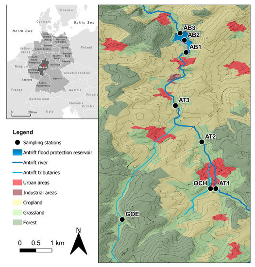
Figure 1.
Location of the Antrift catchment with main water courses and sampling/measurement stations. (Data source: CORINE land use classification by Umweltbundesamt, 2019, DEM 1 m by Hessian Administration for Soil Management and Geoinformation, and overview map according to Weihrauch et al. 2020).
The catchment of the Antrift reservoir has a total area of 61.7 km2 and an altitudinal difference of 152 m from the higher southern parts to the lower northern area. The population ranges between 49–69 persons/km2 (Hessian average: 269 persons/km2). The catchment is a rural region [27] composed of ca. 7.9% settlement area, 45.6% forest, and 45.2% agricultural areas (53.0% cropland and 47.0% grassland) [27,28]. Its landscape is shaped by geological and pedological features (i.e., suitability for land use; Table 1). Forests are mainly found on wooded hills and ridges, where Cambisols and Leptosols (WRB classification) developed from Tertiary alkali basalts or red Mesozoic sandstones. Agricultural lands are largely situated in moderately sloping terrain on Luvisols, Stagnic Luvisols, and Anthrosols developed from Pleistocene loess. Grassland can largely be found in the floodplain areas and valley floors on Gleysols, Gleyic Fluvisols, and Anthrosols developed from Quaternary alluvial sediments [29,30,31,32,33]. Wooded areas are used for forestry, and grassland for grazing [28]. The farms mainly produce wheat, winter wheat, and barley. Out of 67 agricultural holdings, only five practice organic farming [27].

Table 1.
Environmental characterization of the Antrift catchment.
The Antrift catchment comprises the main river Antrift, with a length of 16.5 km, and the headwaters Göringer Bach (11.0 km) and Ocherbach (10.0 km) [34]. Both headwaters join with the main river before it flows into the Antrift reservoir (Figure 1). North of the reservoir, the Antrift river continues to drain towards the Weser River, which finally flows into the North Sea.
The Antrift reservoir has an average water surface of 0.31 km2 and a maximum depth of 10.0 m [35]. It has been characterized as carbonatic and polymictic, with an unstratified water column throughout the year (except for May 2015) [35]. While construction began in 1971, the reservoir was first used for water retention in 1981 [34]. Besides flood protection, it was initially planned to be used for recreational activities and swimming. However, this has never been realized due to strong eutrophication, frequent algae blooms, and fish kills since the 1980s [34]. In 2015, the Antrift reservoir was classified as being in a poor ecological state (polytrophic) according to the European Water Framework Directive [35,36]. High TP concentrations of 0.14 mg TP/l were already measured at the reservoir’s inlet [35], indicating that the local eutrophication issue was catchment-based instead of solely reservoir-based.
The poor ecological status of the Antrift reservoir has remained unexplained to the present day. Several official assessments were carried out to develop effective strategies for water quality improvement. In line with the research history, the eutrophication of the Antrift reservoir was first attributed to P inputs from point sources [1,34,37,38]. However, eutrophication recurred after the only wastewater treatment facility of the catchment had been closed in 2002 (personal communication, F. Reissig, Regional Administrative Council Giessen). Since then, erosion and surface runoff have been considered the major sources of P inputs [37,39,40,41], even though Grimm et al. (2000) concluded in their assessment that only few agricultural lands in the Antrift catchment were severely threatened by erosion [42]. Moreover, erosion has been alleviated further due to financial support and far-reaching advice to farmers, with regard to conservation tillage, intercrop cultivation (especially in winter), conversion of arable lands into permanent grassland, as well as the establishment of vegetated buffer strips along surface waters [20,21]. Since the implementation of erosion conservation measures, the ongoing eutrophication of the Antrift reservoir has been increasingly attributed to P-containing sediment in the catchment water bodies, from which P can be desorbed [37,43,44]. As the impacts of erosion are rather small in this catchment [42], there might not be much sediment in the water courses from which P could be desorbed continuously in an extent large enough to lead to poor ecological state. With regard to legacy P [43], we presume a relatively quick equilibration between P-containing sediments and the water column took place after sediment deposition. This is suggested by Cornel et al. (2015), who showed in a desorption experiment that 20% of the mobilizable P from solids within the effluents of waste-water treatment plants (with Fe and Al precipitation to eliminate P) were set free within a few minutes, and 50% were mobilized within two days [45]. Hence, as sediment deposition has been largely controlled in the Antrift catchment since the 1990s, we do not assume P release from prior sediments to be still relevant today. Thus, theoretically, it is difficult to attribute the present eutrophication of the Antrift reservoir to the P sources commonly discussed in the scientific literature.
3. Material and Methods
3.1. Water Sampling and Water Quality Analyses in the Field
To depict the temporal development of water quality in the Antrift catchment, we determined water quality parameters via field measurements and laboratory analyses of water samples. Our evaluation is based on threshold values and quantitative recommendations for a good ecological status of water bodies given in the “Oberflächengewässerverordnung”, a national regulation implementing the guidelines of the EU Water Framework Directive (WFD) [46]. Water sampling and field measurements were performed in a three-week interval from 5 November 2018 until 6 August 2019 (i.e., 14 sampling/measurement dates). Samples were taken from eight sampling stations in the Antrift catchment (Figure 1, Table 1). GOE and OCH represent the two main headwaters of the Antrift river and pass through forest areas. AT-1 represents the upper reaches of the Antrift river, and AT-2 was chosen because of its location downstream from the major settlement. AT-3 is situated downstream of the tributary Göringer Bach (GOE) and represents the central agricultural area of the catchment. Finally, we chose three sampling stations inside the Antrift reservoir, located at the inlet (AB-1), in the shallow water near the bank of the main reservoir (AB-2), and in the deepest section of the reservoir at the overflow construction of the dam (AB-3).
On each sampling date, three water samples were taken per sampling station from 10–30 cm below the water surface. For GOE, OCH, AT-1, AT2, and AT-3, samples were taken along the channel line. The stations within the Antrift reservoir (AB-1, AB-2, AB-3) were sampled at 3 m distance from the shoreline. Water samples were filled into PE-flasks and kept frozen until further analyses were performed [47].
The field measurements of water quality parameters were performed with an automatic water quality logging system during water sampling (portable logging multiparameter system, HI98290, Hanna Instruments Inc., Woonsocket, RI, USA). The system was operated with the following sensors and accuracies: temperature sensor (°C, ± 0.15), HI7609829-1 sensor for pH (pH, ± 0.02), and HI7609829-2 sensor for DO (%, saturation and concentration, ± 1.5% and ± 0.10 ppm, respectively). The sensor setup was calibrated through autocalibration with standard solutions (Hanna Instruments Inc.) before each measurement date [48]. Temperature, pH, and DO were measured during the whole investigation period.
3.2. Determination of Total Phosphorus in Water Samples
In the laboratory, total phosphorus (TP) was determined according to DIN EN ISO 6878: 2004-09 (2019). Prior to analysis, water samples were unfrozen, brought to an ambient temperature, and mixed with 1 ml 17.97 M sulfuric acid (H2SO4) to adjust pH to ~1. Samples were then oxidized with potassium persulfate (K2S2O8), while heating to 90–100 °C for 90 minutes in closed vessels [49]. Afterwards, extracts were filtered with ashless blue ribbon filters (2 µm pore size). The extracts’ concentration of phosphate was determined on a spectrophotometer (Genesys 10S; Thermo Fisher Scientific; Bremen, Germany) via the molybdenum-blue method at 700 nm [50,51]. Samples were measured three times and averaged. Phosphate concentrations were arithmetically converted into mg TP/l.
We calculated the relative standard deviations of the method (RSDM) and the detection limits for colorimetric TP measurement [52,53,54]. Data below the detection limit were excluded from data evaluation. In our 14 measurements, the maximum RSDM was 4.07%. Hence, we interpret our TP concentrations with a rounded uncertainty range of ± 5.0%.
3.3. Sediment Analyses
We took sediment samples from the water courses in the Antrift catchment to assess potential correlations between water quality parameters and sediment features, especially with regard to P mobilization from sediments. The sediment sampling sites correspond to the water sampling sites (Figure 1). Sediments were sampled about 5–10 cm deep from the bottom of the rivers and the reservoir with a plastic receptacle attached to an extensible stick. The first sampling date (5 November 2018) was in the end phase of a summerly algae bloom after a prolonged period with warm, dry weather and low flow conditions (average in the week before sampling: 0.22 m3/s). The second sampling date (15 March 2019) was after an expected regeneration of water quality during winter. Even though the winter of 2018/2019 was relatively mild and dry, some precipitation occurred prior to our second sampling. Thus, the second date marks relatively moist weather and higher flow conditions (average in the week before sampling: 1.03 m3/s). Sediment samples were stored airtight in plastic bags for about one day until further processing in the laboratory. The sediments were then dried at 70 °C in a drying furnace for eight days. Afterwards, they were ground in a mortar and sieved (2 mm mesh).
We determined the content of organic matter (OM; via loss on ignition; DIN 19684–3:2000–08) and pH (with 0.01 M CaCl2; m:V = 1:2.5; DIN ISO 10390:1997-05) of the prepared samples. Furthermore, we assessed the sediments’ texture with the integral suspension pressure method [55] after samples were prepared according to DIN ISO 11277:2002–08. We used three aliquots of each sediment sample for a P fractionation. We determined the following: (1) easily soluble P with 0.1 M hydrochloric acid (PdHCl) [56]); (2) pedogenic oxide-bound P soluble in an ammonium oxalate–oxalic acid solution (Pox; DIN 19684–6:1997–12 [56]); and (3) pseudo-total P (PAR) after extraction with aqua regia (12.1 M HCl and 14.4 M HNO3 in a ratio of 1:3; [56]). PdHCl was measured on the spectrophotometer according to Murphy and Riley (1962) [48]. Pox and PAR were quantified with an ICP-MS (X Series 2; Thermo Fisher Scientific; Bremen, Germany), as well as Feox, Alox, Mnox, FeAR, AlAR, MnAR, NaAR, MgAR, KAR, and CaAR. All data were converted into the unit mg element/kg. The results of the three aliquots were averaged for further evaluation.
We calculated RSDM and the detection limits for ICP measurement of each element [52,53,54]. Data below the detection limits were excluded from evaluation. Data measured with a relative standard deviation (RSD) of ≥20% were also excluded [57,58]. To quantify measurement uncertainty, we added RSDM (as a standard parameter of calibration-based measurement) with RSD (as a parameter depicting data reproduction, and reflecting effects of heterogeneous matrixes typical for environmental samples [59]). As our sediments were measured in one calibration, only one RSDM resulted for each element. From the several RSD calculated during this measurement, we chose the median RSD for each element, because it is insensitive to outliers. In sum, we calculated rounded-up measurement uncertainty ranges of ± 2.0% (Pox, PAR, Alox, AlAR, Feox, FeAR, CaAR, KAR, NaAR, MgAR), ± 3.0% (Mnox, MnAR), and ± 9.0% (PdHCl).
3.4. Discharge and Precipitation Datasets
At the inlet of the Antrift reservoir, there is a gauging station operated by the Wasserverband Schwalm e.V. (Schwalmstadt, Germany), which measured daily means of flow (m3/s) during our investigation period. Because there is no climate station in the Antrift catchment, average daily precipitation and air temperature were calculated based on data from three climate stations close to the catchment (7–16 km off). These stations were Neustadt (Station-ID: DWD3516, 257 m a.s.l.), Alsfeld-Eifa (Station-ID: DWD91, 300 m a.s.l.), and Meiches (Station-ID: HLNUG4288360, 467 m a.s.l.). The stations are operated by the German Weather Service (DWD) and the Hessian Agency for Nature Conservation, Environment and Geology (HLNUG) [60,61]. All climate data are freely available online.
3.5. Statistical Analyses
Basic statistical operations were performed in Microsoft Excel 2013 (Microsoft; Redmond, WA, USA), in R (R Core Team, 2013) and RStudio (Version 1.1.447; RStudio Inc.; Boston, MA, USA). Data visualization, tests for normal distribution (Shapiro–Wilk test), and Spearman correlation analyses were conducted with the R-packages “graphics”, “stats”, and “corrplot” [62,63]. Significances were tested on different levels. We interpret significant (p ≤ 0.05) correlation coefficients as: weak (rSP 0.4–<0.6), clear (rSP 0.6–<0.8), and strong (rSP ≥ 0.8) [64]. For the sediment data, we performed Spearman correlation analyses for all our data, as well as separately for the data of each sampling date.
Each of our P fractions was determined for a new aliquot (i.e., 1.0 g) of the respective sediment sample. Hence, the resulting P contents are cumulative and contain P forms of different solubility (i.e., Pox includes PdHCl, and PAR includes Pox). To deduce the reactive behavior of sediment P, we calculated differential P fractions, which represent only one class of similar P solubility. Next to easily soluble PdHCl, we calculated moderately labile Pml (Pox minus PdHCl), and recalcitrant Prc (PAR minus Pox).
To depict tendencies in the reactive behavior of sediment P, we determined the degrees of P mobilization (DPM). These ratios between two differently soluble P fractions elucidate whether the sediment has a tendency for P mobilization (large DPM) or P bonding (small DPM [59]). We calculated DPM2 via PdHCl: Pox, and DPM3 via Pox: PAR.
The poor ecological status of the water courses of the Antrift catchment is largely attributed to erosion and overland flow [65,66,67]. Hence, there should be P inputs into the surface waters shortly (i.e., maximally within a few hours) after precipitation events with sufficient intensity [68,69,70,71]. Thus, we used our limited dataset to seek an indication of temporal relationships between TP concentrations in the water and the occurrence of precipitation events. We applied a three-step data evaluation: (1) we tested for similarities between the time series of precipitation and discharge, as a function of the increments of precipitation relative to discharge (“cross correlation”; p ≤ 0.05) [62], to find out if there is a temporal connection between a precipitation event and a discharge event, and to elucidate how quickly the first affects the later. (2) Next, we performed a Spearman correlation analysis between TP concentrations in the water and the number of days between each precipitation event and the next sampling date. For this, rainfall events were classified according to the daily precipitation sum into heavy (>10 mm/day), and maximal precipitation (maximal daily precipitation sum during each three-week measurement period). Moreover, we determined “higher precipitation” for events with a daily precipitation sum between the third quartile and the maximum of each three-week measurement period. Because we wanted to investigate the (short-term) effects of precipitation on erosion and P loss, we picked the “higher precipitation” event that occurred closest to our measuring date. (3) Finally, we checked the absolute number of days between each precipitation event and the next sampling date to evaluate the correlation results and exclude all events which are backdated more than two days. This two-day threshold was chosen according to the results of step (1) and the normal duration of erosion or overland flow events [68,69].
4. Results
4.1. Evaluation of Climate Data: Discharge and Precipitation
According to data from the climate station Alsfeld-Eifa (ca. 7 km northeast of the Antrift reservoir), the last six years show a positive temperature deviation between 0.29 °C and 1.30 °C from the reference period 1991–2020 (Figure 2) [72]. Between 2009 and 2019, the highest positive temperature increase was documented in 2018. A strong negative deviation in annual precipitation sums was reported. Precipitation was ca. 19% lower in 2018 (−135.75 mm), and ca. 10.5% lower in 2019 than in the reference period (1991–2020).
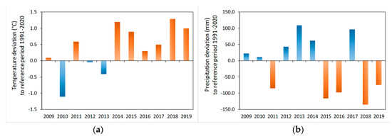
Figure 2.
Temperature (a) and precipitation trend (b) in the Antrift catchment (2009–2019). (Data source: HLNUG (2019); operator: Deutscher Wetterdienst, data for the climate station Alsfeld-Eifa, station-ID: DWD91, 50.7447° N, 9.345° E.).
Between July and November 2018, monthly precipitation sums were lower by between 17.8% (August) and 38.3% (November), compared with the long-term (1979–2020) average monthly precipitation sums (Figure 3). Except for March and May 2019, monthly precipitation sums were below the long-term average precipitation sum all through our field measurement and sampling campaign. The clear increase of the precipitation sum in May 2019 (74.7% higher than in April 2019) resulted from a thunderstorm event with heavy rainfall on 20 May 2019 (Figure 4) [73]. For that day, a 24-h precipitation sum of 45.21 mm was calculated on the basis of data from three regional climate stations (see Materials and Methods). During our investigation period, eleven events with precipitation of >10 mm per day occurred.
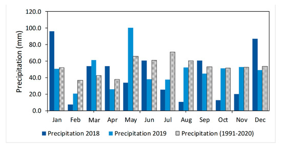
Figure 3.
Monthly precipitation sums in the Antrift catchment during the investigation period, compared to long-term average monthly precipitation (reference period 1991–2020). (Data source: HLNUG (2019); operator: Deutscher Wetterdienst, data for the climate station Alsfeld-Eifa, station-ID: DWD91, 50.7447° N, 9.345° E.).
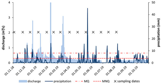
Figure 4.
Monthly precipitation and discharge trend of 2018 and 2019 in the Antrift catchment, compared to average discharge in the reference period 1991–2000 (MQ = average discharge; MNQ = average low-flow discharge). Data source for discharge: Wasserverband Schwalm e.V. (2019), water level station 42881009, 50.76245° N, 9.20654° E. Precipitation data triangulated from HLNUG (2019): climate stations DWD3561 (50.8494° N, 9.1253° E), DWD91 (50.7447° N, 9.345° E), and HLNUG4288360 (50.6281° N, 9.26143° E).
Discharge remained below its long-term average (MQ), with the exception of a few increases in discharge during the winter of 2018/2019, and as a result of the precipitation events previously mentioned (Figure 4). Discharge was low from late spring to summer 2018 and 2019 (data not shown). Except for the weeks with higher rainfall, daily discharge declined below the long-term average of lowest discharge (MNQ).
4.2. Water Quality Assessment
4.2.1. Water Temperature
During the investigation period, water temperature rose steadily from winter to summer (Figure 5a). The increase in water temperature corresponds to the temporal development of air temperature, which only collapsed shortly in May 2019 due to a thunderstorm (see Supplementary Materials) [72]. During winter (December 2018–March 2019), the maximum water temperatures indicated good ecological status. The threshold for poor ecological status (20 °C) was reached in July and (locally) during the following months.
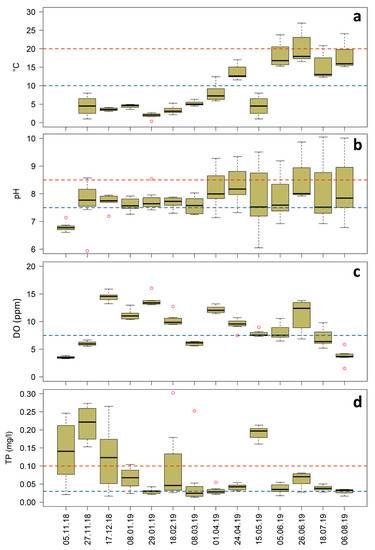
Figure 5.
Time series of water quality data (n = 8 per date). Dashed lines represent thresholds for good ecological status according to OGewV (2016): (a) water temperature, winter maximum (blue line), and summer maximum (red line); (b) pH, minimum (blue line) and maximum (red line); (c) dissolved oxygen (DO), minimum; (d) total phosphorus (TP), threshold between good (<0.03 mg TP/l) and moderate ecological status (>0.03 mg TP/l; blue line), threshold between moderate and poor ecological status (>0.1 mg TP/l; red line).
In the Antrift reservoir, maximum water temperatures ranged between 24.4 °C (26 June 2019) and 21.6 °C (5 June 2019), whereas the temperatures in its tributaries were ca. 6.3 °C lower on these dates (Figure 6a). Since February 2019, the water temperature has been higher in the Antrift reservoir than in the headwaters and the main river. During this time, median water temperatures ranged below the threshold for good ecological quality. Single values, mainly recorded at station AB-2 and AB-3 inside the Antrift reservoir, exceeded the threshold during summer.
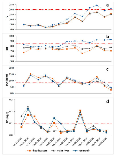
Figure 6.
Temporal trends of water quality parameters during the investigation period; means according to types of water bodies (headwaters (n = 2): GOE, OCH; main river (n = 3): AT-1, AT-2, AT-3; reservoir (n = 3): AB-1, AB-2, AB-3). Dashed lines represent thresholds for good ecological status according to Bundesministerium der Justiz und für Verbraucherschutz (2016): (a) water temperature, summer maximum; (b) pH, maximum; (c) dissolved oxygen (DO), minimum; (d) total phosphorus (TP), threshold between moderate and poor ecological status (0.1 mg TP/l).
4.2.2. pH
Our investigation period started with low surface water pH (6.8–6.9; 5 November 2018; Figure 5b and Figure 6b). All our pH data of the first measurement date, as well as single outliers in the following periods, were within the range for good ecological status [46]. Since April 2019, the pH values inside the Antrift reservoir have been exceeding the threshold for good ecological quality until the end of the investigation period.
With incipient precipitation in late November 2018, pH increased all over the catchment and remained between pH 7.5–8.5 until March 2019. Since March 2019, pH was significantly higher (mean: + 1.5 pH) in the Antrift reservoir than in the main river and headwaters. The lowest pH was recorded in the headwaters, ranging by about 1.9 pH units under the reservoir pH.
4.2.3. Dissolved Oxygen
Our DO data show no clear trend (Figure 5c and Figure 6c). Generally, DO concentrations increased after a minimum in November 2018 (mean: 4.8 ppm) to stay above the threshold for good ecological status (8 ppm DO). Between July and August 2019, DO concentrations clearly decreased in the headwaters and the main river (80.3% and by 61.0%, respectively), compared to DO concentrations in June. The minimum DO concentrations in August 2019 ranged between 2.57 ppm in the headwaters and 4.52 ppm inside the reservoir. No significant spatial variability of DO concentrations was found for the Antrift catchment (Figure 6c). However, headwaters had slightly higher DO concentrations at single measurement dates.
4.2.4. Total Phosphorus
The TP concentrations were relatively high, varied strongly, and indicated bad ecological status in the investigated water courses (Figure 5d). During November and December 2018, TP levels remained high (>0.10 mg TP/l). From February 2019 to August 2019, lower TP concentrations were recorded, ranging between the lower and upper thresholds of eutrophic nutritional status. However, outliers occurred with >0.25 mg TP/l. The largest outliers were found at station AB-2 (reservoir), with 0.30 mg TP/l (18 February 2019) and 0.25 mg TP/l (3 March 2019). In May 2019, a single increase was detectable to TP concentrations of >0.20 mg TP/l. We found no systematic spatial trend of TP concentrations in the catchment despite slight differences between the hydrological water body types (Figure 6d and Figure 7).
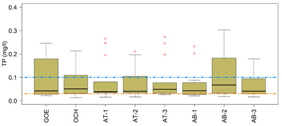
Figure 7.
Total phosphorus (TP) concentration during the investigation period, according to sampling stations (n = 14 per station). Dashed lines represent thresholds of nutritional status according to OGewV (2016): orange line = threshold between good (<0.03 mg TP/l) and moderate ecological status (>0.03 mg TP/l); blue line = threshold between moderate and poor ecological status (>0.1 mg TP/l).
4.3. Correlation of Total Phosphorus Concentrations and Precipitation Events
The cross correlation between the time series of precipitation and discharge data shows a significant (p ≤ 0.05) mutual influence for a period from 0 to ± 2 days (see Supplementary Materials). Within this two-day period, the results of the auto correlation function (ACF) were above the 0.1 ACF threshold. At point zero (i.e., precipitation and discharge event on the same day), the highest ACF value (0.416) is reached, followed by a continuous decrease until point +2 (i.e., discharge event two days after precipitation event).
Based on this result, Spearman correlation analyses (Figure 8) show a strong and significant (p ≤ 0.05) positive correlation between the number of days since the last high, maximum, or heavy precipitation event (˃10 mm/day) and the maximal drainage for each measurement period.
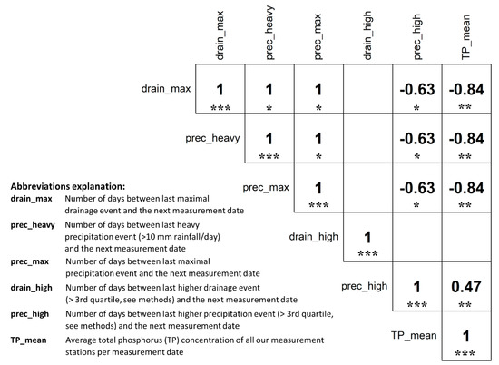
Figure 8.
Spearman correlation coefficients of TP concentrations in the water and the number of days between each precipitation event and the next sampling date. (Significance levels: p ≤ 0.001 (***); p ≤ 0.01 (**); p ≤ 0.05 (*)).
Comparing the average TP concentrations with the number of days since the last maximal drainage or maximal and heavy precipitation events, a strong significant (p ≤ 0.01) negative correlation was found. Moreover, a moderate positive correlation was observed between average TP and the number of days since the last higher precipitation event. Instead, no significant correlation was found for TP and the number of days since the last higher drainage event.
Beside these results of the correlation analyses, the absolute number of days since an event was mostly larger than two days for all the precipitation events during our investigation period (see Supplementary Materials). Only in August 2019 did a maximal precipitation event coincide with our sampling date. For higher precipitation, six of 14 measurement periods showed an event within two days. No heavy precipitation event occurred within the two-day interval.
4.4. Sediment Analyses
4.4.1. General Sediment Features
The sediments from the Antrift catchment were largely silty-loamy (average: 63.9 mass-% silt, 18.1 mass-% sand, 18.0 mass-% clay; Table 2). However, the clay content decreased and the sand content increased from the headwaters (25.7 mass-% clay, 5.5 mass-% sand; averages) to the reservoir (16 mass-% clay, 27.3 mass-% sand; averages). The silt content decreased slightly from the headwaters/main river (mean: 68.7 mass-%) to the reservoir (mean: 56.7 mass-%). There was also temporal variation in the sediments’ textures from the first to the second sampling (average deviations: +6.2 mass-% silt; +9.3 mass-% sand, −15.5 mass-% clay).
Table 2.
General sediment features.
With an overall mean pH of 6.8, the sediments depict slightly acidic to neutral conditions. However, over our study period, the catchment pH shifted between slightly alkaline conditions (first sampling) and slightly acidic conditions (second sampling). The average pH increased from the headwaters (slightly acidic), to the main river, to the reservoir (slightly alkaline).
The sediments in the Antrift catchment were relatively high in organic matter (OM; overall mean: 8.6 mass-%). There was a slight tendency for OM contents to decrease from the headwaters to the main river to the reservoir at the first sampling (17.1 vs. 7.9 vs. 4.7 mass-%, respectively). However, OM contents were relatively similar at the second sampling (8.3 vs. 8.8 vs. 7.4 mass-%, respectively).
4.4.2. Sediment Phosphorus Contents
The sediments in the Antrift catchment are relatively high in each of the determined P fractions (Table 3). We found spatial and temporal variability in the sediment P data. The average PdHCl contents were significantly larger at the second sampling (+30.3%). Besides, we found relatively large ranges of the PdHCl means of the hydrological units. Through our study period, the largest mean PdHCl occurred in the main river stations. However, for the first sampling, the smallest mean PdHCl was in the reservoir. On the second date, the minimum average PdHCl was instead observed in the headwaters.
Table 3.
Differential P fractions and degrees of P mobilization of sediments (means).
The Pml contents changed insignificantly from the first to the second sampling (+26%) and among the hydrological units. However, there was an increase in Pml in the headwaters and the reservoir at the second sampling. The mean Prc contents also increased in the reservoir at the second sampling, but decreased in the headwaters. The largest mean Prc contents were generally found in the main river.
We found relatively large DPM2 and DPM3 (i.e., >0.4). From the first to the second sampling, DPM2 remained constant in the main river. It was extremely small in the reservoir at the first sampling, but almost doubled to the second sampling. By contrast, DPM2 decreased by about 33% in the headwaters from Sampling 1 to Sampling 2. DPM3 increased slightly to the second sampling (+19%). However, we found no significant changes between the sampling dates and hydrological units.
4.4.3. Correlation Analyses
We conducted Spearman correlation analyses for all our data, as well as separately for the data of each sampling date. Different correlation coefficients result in these three versions of data aggregation. The specific results for the correlation of all data are shown in Figure 9. However, we also found overarching correlations (i.e., present in all three versions of data aggregation).
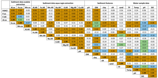
Figure 9.
Spearman correlation of sediment and water data for both samplings. p ≤ 0.05 (green), p ≤ 0.01 (blue) and p ≤ 0.001 (brown), not significant (no color).
First, there are regular correlations between the moderately labile to recalcitrant P fractions and the acid metal cations, as well as the base cations. PdHCl, Pox, and PAR are correlated positively and clearly to strongly with Alox, AlAR, FeAR, NaAR, MgAR, CaAR. For all data, there are furthermore positive correlations of PdHCl, Pox and PAR with Feox (weak) and KAR (weak to clear; Figure 9).
Second, we mostly found weak positive correlations of PdHCl, Pox, and PAR with the sediments’ OM content.
5. Discussion
5.1. Evaluation of Climate Data: Discharge and Precipitation
The trends of air temperature and monthly precipitation showed uncommonly warm and dry conditions in the Antrift catchment in 2018 and 2019 (Figure 2). These years could be termed ‘extreme’, regardless of the general trend for precipitation to decrease on average by 68 mm per decade in Hesse [22,72]. Despite the long-term drought, increased heat and low flow conditions, individual higher to heavy precipitation events occurred during the investigation period, whose rainfall intensity might have enabled soil erosion [68,74]. However, a high potential for causing soil erosion can only be attributed to the storm event on 20 May 2019, which exceeded a daily precipitation sum of 70 mm, and could hence be termed an extreme rainfall event [68,74,75]. Such extreme weather conditions are assumed to increase in frequency under climate change [16].
Climate forecasts (e.g., IPCC, HLNUG) predict an increase of annual mean temperature, heat extremes, drought periods, and heavy precipitation events [25,26,76]. We documented all these factors during our investigation period. Therefore, our data are likely to draw a picture of water quality impairment under climate change.
5.2. Water Quality Assessment
5.2.1. Water Temperature
In general, water temperature is correlated with air temperature. An increase in air temperature through climate change leads to increasing water temperatures [16]. In addition, water temperature is a main factor controlling chemical and physical properties of aquatic ecosystems (e.g., pH, diffusion rates) [2,14]. The water temperature within the Antrift reservoir and its tributaries ranged between the lower and upper thresholds for good ecological status during our investigation period. Although a moderate increase of air temperature from winter to summer was detected (see Supplementary Materials), the influence of climate change and a long-term increase of water temperature could not be investigated, because this study considers a 10-month period only. However, a long-term increase in water temperature is documented for rivers and lakes by other studies and can be assumed for the Antrift catchment under aggravated climate change conditions [5,77]. Deviations from the moderate annual increase of water temperatures from spring to summer occurred only due to heavy rainfall events (e.g., a thunderstorm in May 2019). Moreover, minor differences were observed due to spatial variation between lower water temperatures at sampling sites shaded by riparian vegetation (e.g., headwaters, the main river) and higher temperatures in the unshaded Antrift reservoir.
Water temperature and sufficient nutrient concentrations stimulate algal growth [1]. To do so, temperatures were too low (<20 °C to 23.0 °C) at the beginning of our measurement period [77,78]. Climate change is projected to increase the persistence of high water temperatures—especially in shallow lakes—and thus lead to extended eutrophication periods and algal blooms [2,16,17]. However, Richardson et al. (2019) observed factors limiting total phytoplankton growth and fostering the decrease of harmful cyanobacteria in nutrient-rich environments. Thus, climate change effects on algae blooms might be more complex than commonly assumed [79].
In our study, temperatures have been favorable for algal growth since June 2019. On 5 June 2019, an incipient bloom of blue-green algae was observed, leading to a widespread green-brown algal carpet on the water surface of the Antrift reservoir in August 2019 (see Supplementary Materials). At the Antrift main river and the headwaters, no such visible water quality impairment was observed, probably due to more riparian shading and higher flow velocity [80,81].
5.2.2. pH
On 5 November 2018, pH in the Antrift catchment was relatively low (Figure 5b), probably as a result of the bacterial degradation of the 2018 algae bloom [1,15]. During the winter period, pH oscillated around the lower threshold (7.5 pH) for good ecological quality. Beginning in April 2019, pH rose to a more alkaline level [2]. The high fluctuation (i.e., range) of pH is typical for increasing eutrophication appearances [1,82,83]. At that time, we observed increased biomass formation in the reservoir. A second decrease of pH in connection with biomass increase was not observed, because our investigation period ended in August 2019.
5.2.3. Dissolved Oxygen
Despite the three-week interval between measurements, two trends in DO were observed. First, both algae blooms (end phase in November 2018, build-up in June 2019) were correlated with low DO concentrations. The minimum DO concentrations were measured during the end of the 2018 algae bloom, probably resulting from oxygen depletion through the intensified bacterial degradation of biomass [1,84,85]. Hence, after the winter increase, DO concentrations decreased again after August 2019, when the 2019 algae bloom had already built up for at least two months. Second, increases in DO coincided with increases in precipitation and discharge after the long drought phase in the second half of 2018. Increasing flow velocity leads to a higher level of DO in the surface waters [13,86]. Hence, during winter and spring 2019, DO stayed above the threshold for good ecological status.
The spatial differentiation of DO concentrations reflects the water temperature differences between the reservoir, the main river, and the headwaters [87]. Higher DO concentrations occurred at the headwater stations on single dates, probably as a result of higher flow velocity and shading by riparian vegetation (see Supplementary Materials). Still, during the 2019 algae bloom, the lowest DO concentrations were measured in the headwaters, most likely because of low flow rates and low velocity [88,89]. This indicates a higher vulnerability of the headwaters for water quality impairment under climate change (e.g., due to prolonged low flow conditions).
5.2.4. Total Phosphorus
Our data confirm that the Antrift reservoir is eutrophicated according to the EU Water Framework Directive. High TP concentrations occurred throughout our investigation period (Figure 5). However, TP concentrations indicating poor ecological quality were measured only from November to December 2018, and sporadically (event-driven) in February and May 2019. On the one hand, the high TP concentrations between November and December 2018 can be explained by low flow rates and a low nutrient dilution in the water column [16]. On the other hand, this period marks the end phase of the 2018 algae bloom with low DO concentrations and pH.
The average TP concentrations decreased continuously until January 2019. This can be attributed to the increase in precipitation and flow rates within the Antrift catchment. Even with the relaxation of the eutrophication situation during winter 2018, the median TP concentrations stayed close to the lower threshold of eutrophic conditions (except for single outliers; Figure 5d). After the autumnal decrease, TP concentrations varied slightly for the rest of the studied period.
Since July 2019, there was a strong negative correlation of TP concentrations with water temperature (rSP = −0.66; p = 0.01). On 5 June 2019, the water temperature reached the 20 °C-threshold favorable for algae growth. As a consequence, the TP concentrations decreased, suggesting a consumption of P. This decrease of TP is corroborated by our field observations of increasing algal growth, which was also documented in other case studies [67,90].
With regard to our sampling stations, some conclusions can be drawn regarding potential P sources. We found no increase in TP concentrations with increasing percentage of agricultural land use or settlements [65,91,92]. Interestingly, TP concentrations are somewhat lower in the headwater stations than in the main river and reservoir, but they are still within the range of eutrophic nutritional status.
The reservoir and both stream classes are clearly different in hydrology and morphology. However, no significant difference in stream morphology is assumed between the headwaters and the main river [67]. Generally, our TP data mostly depict no clear differences between the three types of surface water bodies. Thus, not only is the Antrift reservoir eutrophicated, but all the investigated water bodies in the catchment, even the headwaters, are. This indicates that agriculture (erosion, surface runoff) and settlements (point sources) should not be termed the major factors for causing eutrophication in the Antrift catchment. Because the headwater station GOE is situated in a forest region, high TP concentrations also occur in areas without erosion risk and point sources (see Supplementary Materials). Hence, there seem to be further, so far unnoticed, sources for P losses from soil to water.
The TP trend, in combination with the trend of water temperature, pH, DO, and field observations, indicates that, under climate change, the relaxation of water quality impairment during winter could be shortened. Our data depict an extended duration of the 2018 algae bloom and a new worsening of water quality in April 2019. P stocks conserved from the prior algae bloom could accelerate the next algal bloom in spring. This is corroborated by Richardson et al. (2019), who showed that an increase in water temperature, sufficient nutrient levels, and hydrological conditions (e.g., intensive precipitation after drought events) might trigger cyanobacteria growth and complex algal bloom dynamics [79].
5.3. Phosphorus Sources in the Antrift Catchment
After the only wastewater treatment plant closed in 2002, no major point sources for P inputs remained in the Antrift catchment [93]. Erosion and surface runoff are thus expected to be the major P sources due to the large percentage of agricultural lands (>45%) [27]. However, the local erosion risk has been judged low in an official assessment [18,68]. Besides, vegetated buffer strips have been established along the water courses in the catchment, even along smaller drainage channels. Moreover, the influence of direct surface runoff and drainage must be considered minor, as a result of the very limited proportion of sealed surfaces.
We tested the influence of possible P inputs by erosion and surface runoff, with a correlation analysis between TP concentrations and their occurrence (i.e., number of days) after the last precipitation event (see Section 3.5. Statistical Analyses). The cross-correlation between the time series data of precipitation and discharge shows that precipitation events influenced the discharge trend significantly (see Supplementary Materials). This correlation is significant for a range between 0 and +2 days after rainfall events. Precipitation events thus had a significant impact on runoff in water bodies for a maximum of two days after the respective event.
The Spearman correlation analyses resulted in a significant negative correlation between average TP concentrations and the number of days since different kinds of precipitation events (Figure 8). Thus, a larger number of days since the last precipitation event coincided with lower TP concentrations in the water bodies. This indicates an influence of precipitation events and intensity on the TP concentrations (e.g., erosion and surface runoff) [71,93]. However, both processes are short-term processes, with a potential direct impact on water quality within a few minutes to hours, maximally in <2 days [68].
During our investigation period, no precipitation event occurred so shortly before a measurement date (i.e., <2 days) that it could be attributed plausibly to erosion or surface runoff [68]. In particular, all the potentially highly erosive higher and heavy precipitation events happened more than two days before our measurements [68,69,70]. Therefore, neither point sources nor extensive erosion (with surface runoff) can be considered as the major reasons for the all-season high P concentrations in the Antrift catchment. Instead, our results might tentatively point to an effect of underground P translocation (interflow-P), with a delay after precipitation events due to water infiltration and percolation [94,95]. However, our approach is limited by the relatively coarse temporal resolution of our measurements (three weeks) [68,69].
5.4. Sediment Analyses
5.4.1. General Sediment Features
The texture of the sediments results from the typical bedrocks and substrata in the Antrift catchment. The dominance of silt probably results from the large spatial extension of loess [29,96]. The somewhat higher clay content in the headwater area could be explained by the abundance of basalt in this section of the catchment. By contrast, the increasing percentage of sand in the reservoir sediments could be due to the occurrence of sandstones in the reservoir’s surroundings. The variation we found between sediment textures of Samplings 1 and 2 generally demonstrates that sediments are dynamic components of the soil-water-interface, which undergo constant changes by transport, selection, and biochemical reactions [97,98]. Those processes could affect the textural composition of the sediments.
Over our investigation period, the sediments oscillated between slightly acidic and slightly alkaline conditions (Table 3). This general pH range can also be attributed to the dominance of alkali basalt and loess in the Antrift catchment [96]. That pH was lower in the headwater area than in the reservoir is probably geochemically determined. The headwaters are surrounded by basalts, which contain relatively many base cations (Ca, Mg, K), but even more Al/Fe (among other elements). Instead, base cations are probably more abundant in the loess areas (main river, reservoir) [96]. Moreover, pH could increase towards the reservoir due to the increasing concentration of leached basic cations, with increasing flow distance through the catchment.
We found the highest variance of pH between our sampling dates in the main river stations. This seems plausible because the main river represents the largest part of the catchment area and hence the most hydrologically diverse conditions [99]. Instead, the headwaters and the reservoir depict relatively small sections of the catchment with rather controlled hydrological conditions [97,99].
That we found large OM contents is not surprising for fluvial and lacustrine sediments, especially with eutrophication-enhanced primary productivity and the increased accumulation of dead OM [1,5]. Our OM contents decrease from the headwaters to the reservoir, which might be due to increased OM mineralization during summerly eutrophication and algae blooms [3]. Moreover, this spatial differentiation of sediment OM might be related to the spatial distribution of land uses in the Antrift catchment. The headwater areas are largely composed of forests, which produce and transfer more OM to the adjacent water courses. The main river and reservoir stations are instead located in agricultural (conventional farming) and grassland areas, where less OM is produced [96].
5.4.2. Sediment Phosphorus Contents
The large sediment P contents might in part result from the bedrocks in the Antrift catchment (e.g., basalt). Besides, they could be the legacy of prior land management (especially in the agricultural areas around the main river stations). However, the build-up of sediment is generally relatively small and also well-controlled in the Antrift catchment since the 1990s [42]. Instead, sediment pH might be a relevant and overarching driver of sediment P in this catchment. The mean pH levels of the sediments were between 6.0 and 6.5. P mobility is large in this pH range [100,101] because the solubility of P-sorbing metal oxides is relatively low (lability increases with pH), while at the same time, P-bearing minerals precipitating with base cations are also relatively easily soluble (stability increases with pH [96,102]). Hence, any shift of pH would foster P mobilization: Under more acidic conditions, the P-bearing minerals of base cations would be dissolved [103,104]; under more alkaline conditions, P would increasingly be desorbed from metal oxides [105,106]. It is a particularity of the Antrift catchment that sediment P retention is governed by sorption to metal oxides and by precipitation with base cations, instead of either of both. Thus, sediment P contents could be large due to the large number of potential reaction partners. However, a decrease in pH might be most favorable for P retention in the Antrift sediments, because metal cations are much more abundant in the sediments than the base cations.
We found larger sediment PdHCl contents at the second sampling. This might result from an increased tendency to Pml mobilization (i.e., conversion to PdHCl) under high flow conditions (high dilution). Such conditions would cause a disequilibrium between bound P in the sediment and dissolved P in the water column [102,107]. As equilibrium would be shifted towards bound P, P mobilization would be enhanced to restore the equilibrium state [108,109].
The differences between the average PdHCl contents at both samplings suggest that the three hydrological units might be subject to different P dynamics, especially under an acute algae bloom. In the reservoir, PdHCl was very low at the first sampling, possibly due to enhanced P mobilization (i.e., loss of PdHCl) during the 2018 algae bloom and severe DO depletion (Figure 5c). Without an acute algae bloom, PdHCl increased significantly at the second sampling. By contrast, PdHCl decreased in the headwaters at the second sampling. This could be the consequence of increased P mobilization under high flow conditions.
The Pml contents increased slightly but non-significantly on the second date. This might suggest a tendency to P mobilization under high flow conditions, which could successively convert recalcitrant P forms into Pml [6]. Even though not statistically significant, Pml increased in the headwaters and in the reservoir. Most likely, in the reservoir, the small Pml content at Sampling 1 resulted from the acute algae bloom and enhanced P mobilization from the sediment. In the headwaters, the increase in Pml might instead have resulted from successive equilibrium-driven P mobilization under high flow conditions [6,107]. This might also explain the decrease in Prc in the headwaters at the second sampling. However, the increase in Prc in the reservoir might also have resulted from a relatively small Prc at Sampling 1 due to the acute algae bloom with severe DO depletion.
The largest Prc contents were generally found in the main river. With regard to the local bedrocks/substrata (loess), this is possibly due to the high abundance of base cations in the water, which can precipitate with dissolved P, especially under low flow conditions (Sampling 1) [96,109]. Moreover, the main river stations are not affected by algae-bloom–enhanced DO depletion and resulting P mobilization from sediments. Hence, more Prc might accumulate
The relatively large DPM2 and DPM3 suggest that the sediments in the Antrift catchment are generally prone for P mobilization due to their large share of readily and moderately soluble P forms. We found slightly larger DPM2 (+19%) and DPM3 (+19%) at the second sampling, which might point to increased P mobilization under high flow conditions. By contrast, the small DPM2 in the reservoir at Sampling 1 might have resulted from algae-bloom-mediated P mobilization.
To the second sampling, DPM2 decreased significantly in the headwaters. Because the lowest pH were observed for the headwaters, there might be more reactions between P and Al/Fe, which are favored under acidic conditions [103,104]. P associated with Al/Fe would raise sediment Pml (based on Pox) [105,106] and thus result in a smaller DPM2. Furthermore, Pml might have increased due to the above-mentioned successive mobilization of Prc.
For DPM3, we found no significant changes between the sampling dates and hydrological units. However, the smallest DPM3 was found in the reservoir on the first date. This might also have resulted from the above-stated tendency for sediment P mobilization under severe DO depletion.
5.5. Spearman Correlation Analyses of Sediments and Water Samples
Our correlation analyses resulted in different relationships between the sediment and water parameters when all our data were combined (Figure 9) or grouped according to sampling dates (Figure A1 and Figure A2). Hence, temporal dynamics of rather short-term processes like acute eutrophication with an algae bloom are probably depicted more adequately as snapshots according to sampling dates instead of sums or averages of longer timespans (e.g., yearly averages [3]).
5.5.1. Correlations with Acid and Base Metal Cations
We found overarching positive correlations of PdHCl, Pox, and PAR with Alox, AlAR, FeAR, NaAR, MgAR, and CaAR. This indicates that P bonding in the sediments is strongly governed by the acid metal cations (especially Al), probably largely via sorption, which the strong correlations with Alox point to [102,103]. The correlations of PdHCl, Pox, and PAR with AlAR and FeAR might furthermore indicate that the precipitation of Al/Fe and P-containing minerals could play a role. However, the correlations of PdHCl, Pox, and PAR with NaAR, MgAR, and CaAR indicate that mineral precipitation, either with instantaneous (e.g., Ca-P-minerals) or with subsequent P bonding (e.g., adsorption and surface precipitation [110,111]), might also be relevant for sediment P retention.
5.5.2. Correlations with Sediment Organic Matter
We found weak positive correlations of PdHCl, Pox, and PAR with the sediments’ OM content. Because OM contains P, an increasing amount of OM also means an increase of the bound P fractions. Furthermore, the mineralization of organic matter leads to P mobilization to the water column and might result in an increase of TP. This is indicated by the weak negative correlation between sediment OM and TP in the water (Figure 9, Figure A1 and Figure A2). However, this correlation is visible only at the second sampling. On the first date, other eutrophication-related processes might instead have controlled TP.
Generally, the relatively large sediment OM contents (average: 8.61 mass-%) might hamper precipitation reactions and favor the formation of more weakly crystalline mineral phases [104,112]. This might explain why we found correlations of the P fractions with sand and silt but not with clay.
Generally, P bonding increases with clay content because most of the major P sorbing particles belong to the clay fraction (e.g., Fe/Al oxyhydroxides, OM [100,113]). However, Weihrauch (2018) found correlations of soil P fractions with sand and silt instead of clay in a study area characterized by weakly acidic to weakly alkaline soils [59]. The author explained this finding with the precipitation of carbonates adsorbing P weakly in a monolayer (at low P concentration) and with the precipitation of rather amorphous Ca-P-minerals (at higher P concentration) of larger diameter, due to the interference with OM [112]. Moreover, P might become occluded in a recalcitrant form within Mn and Fe concretions, which could grow with time [96,114,115]. This might explain the correlations between PAR and sand (Figure 9, Figure A1 and Figure A2). The correlations between sand and PdHCl might instead result from P sorption and surface precipitation on calcite, the formation of easily soluble Ca-P-minerals, and/or amorphous metal oxides [102,116]. Such a P retention in larger particles might also explain the clear negative correlation between the sediments’ silt content and TP in the water (e.g., apatite often forms crystals in the silt fraction [96]). Hence, sediment OM is indicated to affect sediment P contents directly as well as indirectly by influencing the potential P bonding sites.
The above-mentioned correlations show for only the second sampling, probably due to strong effects of eutrophication on P dynamics on the first date. However, we found a strong negative correlation of sediment OM and pH in the water on the first date, which could have resulted from decreasing pH with increasing OM abundance and related mineralization [88,117].
6. Conclusions
We investigated the eutrophication of the Antrift reservoir in Hesse (Germany) in the uncommonly warm and dry years 2018/2019. Our results give an empirical preview on the development of local water quality under climate change. They furthermore enabled us to answer crucial questions regarding the poor ecological status of the Antrift reservoir.
Our results clarify that not only the Antrift reservoir is affected by eutrophication due to high TP concentrations, but so is the entire catchment. The catchment TP concentrations are high throughout the year, but apparently not due to the P sources commonly stated in eutrophication literature (e.g., agriculture). Possibly, natural pH-driven P mobilization from catchment soils and sediments (depending on soil moisture and flow conditions) might foster the eutrophication of the local surface waters. This hypothesis of an “autogenous eutrophication” should be investigated further.
Conceptually, we differentiate between two kinds of constraints on TP concentrations (graphical abstract): biological and geochemical constraints. Biological constraints are largely determined by water temperature, pH, and nutrient availability (especially P). In the Antrift catchment, pH and TP concentrations are favorable for algal growth throughout the year. Hence, temperature might be the major driver of algal growth, DO depletion, and resulting sediment P mobilization in summer. During the winter, water temperatures <20 °C prevent algal growth and DO depletion. Thus, only in summer can biological constraints lead to algae blooms with acute DO depletion. Under such conditions, they outweigh the geochemical constraints.
The geochemical constraints are determined by flow conditions (elemental dilution), water and sediment pH, redox status, as well as, to a lesser degree, by the local bedrocks/substrata (supply of P, Al, Fe, Mn, Ca, Mg, K). At low flow conditions and low dilution (summer), P might increasingly be retained in sediments. By contrast, P is likely to be increasingly mobilized from sediments at high flow conditions and high dilution (winter). This should be studied further.
In the literature, P dissolution/remobilization from sediment mostly describes P desorption/dissolution from sediment that has been transferred to water courses due to land use (especially agriculture) [43,118]. For our argument, it is not relevant where the sediments come from. Sediment P equilibrates relatively rapidly with P in the water column [6]. Hence, any P desorption/dissolution from P-enriched sediment from agricultural lands would likely happen quickly after deposition [45]. Then, the sediments would be subject to the geochemical constraints in the Antrift catchment, which generally foster a high abundance of labile sediment P and temporary P mobilization. This would apply to any sediment, regardless of its original P load and origin regarding land use. Hence, we are skeptical about the scientific theories of a “hysteresis” of P dissolution from sediment, which is sometimes evoked to explain why best-management to improve water quality practices do not succeed right away, but might need decades [43,119].
With regard to climate change, our data from the recent uncommonly warm years corroborate the assumptions of others (e.g., LeMoal et al. 2019; Moss et al. 2011; Whitehead et al. 2009) that global warming will likely foster eutrophication, as well as prolonged and spatially extended algae blooms. Climate change might hence aggravate biological constraints in summer. In winter, however, lowered flow conditions might instead lead to reduced P mobilization, or, in other words, to increased P retention in the catchment sediments. However, combined effects between cyanobacteria and phytoplankton, short-term hydrological changes, and nutrient availability in freshwater ecosystems and sediments might complicate a clear prediction of the interaction of constraints on P mobilization/retention under climate change [79,120,121].
To mitigate the eutrophication of the Antrift catchment, it is important to register that TP concentrations are naturally high throughout the year. Hence, any artificial reduction of TP concentrations (e.g., by common best-management practices) would foster geochemical P mobilization from the sediment. As mentioned above, the Antrift catchment could theoretically self-regulate its ecological status under natural conditions (e.g., by flushing winterly nutrient excesses downstream). The Antrift reservoir undermines this self-regulation and creates an environment of all-year P accumulation in the water column, which artificially fosters algae blooms in summer.
We conclude that the eutrophication (i.e., TP concentrations of 0.03–<0.1 mg TP/l) of the Antrift catchment cannot be prevented. Still, best-management practices should be kept active (e.g., erosion conservation) to prevent further P inputs that could aggravate eutrophication and lead to a poor ecological state (TP concentrations ≥0.1 mg/l). To restrict the summertime P mobilization from the sediment, DO concentrations should be started to be managed besides TP concentrations. Hence, algae blooms (and resulting DO depletion) might be controlled with algicides or the introduction of certain key species into the water bodies [1], bearing in mind the possible ecological consequences. Furthermore, artificial aeration of the Antrift reservoir could significantly relax summerly hypoxia and anoxia. Without hypoxia, the geochemical constraints would probably be dominant in summer and trigger P retention in the sediments. A certain monitoring and the eventual removal of the catchment sediments should also be considered, especially regarding sediments loaded with P in summer. In addition, the respective material would have beneficial features for application as fertilizer (e.g., high in carbonate and OM, pH 6–7, much labile P), if it was free of toxins, etc.
Our study indicates that—beside the known sources of P inputs—there might be currently unknown and unregulated diffuse P sources which contribute to the high P concentrations of the surface waters in the Antrift catchment. These sources seem to depend on the flow conditions, but are activated >2 days after precipitation events. Hence, we hypothesize an underground P translocation with the soil water (interflow-P) [94]. Such P sources should be investigated further so that they could be effectively managed and restricted. Hence, our study demonstrates that freshwater eutrophication is not yet conclusively understood despite the successes in research and practice. Challenges remain for science and should possibly be tackled apart from the disciplinary and conceptual mainstream.
Supplementary Materials
The following are available online at https://www.mdpi.com/2571-8789/4/2/29/s1, Figure S1: Average monthly air temperature for the climate station Alsfeld-Eifa, Figure S2: Pictures of algal bloom in the Antrift reservoir, Figure S3: Stations of water and sediment sampling in the Antrift catchment, Figure S4: Cross-correlation matrix of precipitation and discharge data, Table S5: Days since precipitation/discharge events according to measurement periods.
Author Contributions
Conceptualization, C.J.W., C.W.; Methodology, C.J.W., C.W.; Software, C.J.W., C.W.; Validation, C.J.W., C.W.; Formal Analysis, C.J.W., C.W.; Investigation, C.J.W., C.W.; Resources, C.J.W., C.W.; Data Curation, C.J.W., C.W.; Writing—Original Draft Preparation, C.J.W., C.W.; Writing—Review & Editing, C.J.W., C.W.; Visualization, C.J.W., C.W.; Supervision, C.W.; Project Administration, C.W.; Funding Acquisition, C.W. All authors have read and agreed to the published version of the manuscript.
Funding
This research was funded by the Regional Administrative Council Gießen (Regierungspräsidium Gießen).
Acknowledgments
The authors gratefully acknowledge supply with discharge data by the Wasserverband Schwalm e.V. We furthermore thank Alexander Santowski for support in statistical data evaluation and Christin Wedra for support in laboratory analyses. Finally, we thank our students who partook in the research-based seminar and laboratory courses on the eutrophication of the Antrift reservoir.
Conflicts of Interest
The authors declare no conflict of interest.
Appendix A

Figure A1.
Spearman correlation of sediment and water data for Sampling 1 (5 November 2018). p ≤ 0.05 (green), p ≤ 0.01 (blue) and p ≤ 0.001 (brown), not significant (no color).
Figure A1.
Spearman correlation of sediment and water data for Sampling 1 (5 November 2018). p ≤ 0.05 (green), p ≤ 0.01 (blue) and p ≤ 0.001 (brown), not significant (no color).


Figure A2.
Spearman correlation of sediment and water data for Sampling 2 (15 March 2019). p ≤ 0.05 (green), p ≤ 0.01 (blue) and p ≤ 0.001 (brown), not significant (no color).
Figure A2.
Spearman correlation of sediment and water data for Sampling 2 (15 March 2019). p ≤ 0.05 (green), p ≤ 0.01 (blue) and p ≤ 0.001 (brown), not significant (no color).

References
- Le Moal, M.; Gascuel-Odoux, C.; Ménesguen, A.; Souchon, Y.; Étrillard, C.; Levain, A.; Moatar, F.; Pannard, A.; Souchu, P.; Lefebvre, A.; et al. Eutrophication: A new wine in an old bottle? Sci. Total Environ. 2019, 651, 1–11. [Google Scholar] [CrossRef]
- Nazari-Sharabian, M.; Ahmad, S.; Karakouzian, M. Climate Change and Eutrophication: A Short Review. Engineering. Technol. Appl. Sci. Res. 2018, 8, 3668–3672. [Google Scholar]
- Bowes, M.; Davison, P.; Hutchins, M.; McCall, S.; Prudhomme, C.; Sadowsko, J.; Soley, R.; Wells, R.; Willets, S. Climate Change and Eutrophication Risk in English Rivers; Technical Report No. SC140013/R; Environment Agency: Bristol, UK, 2016.
- Dodds, W.K.; Bouska, W.W.; Eitzmann, J.L.; Pilger, T.J.; Pitts, K.L.; Riley, A.J.; Schloesser, J.T.; Thornbrugh, D.J. Eutrophication of US Freshwaters: Analysis of Potential Economic Damages. Environ. Sci. Technol. 2009, 43, 12–19. [Google Scholar] [CrossRef]
- Charlton, M.B.; Bowes, M.J.; Hutchins, M.G.; Orr, H.G.; Soley, R.; Davison, P. Mapping eutrophication risk from climate change: Future phosphorus concentrations in English rivers. Sci. Total Environ. 2018, 613, 1510–1526. [Google Scholar] [CrossRef]
- Correll, D.L. The role of phosphorus in the eutrophication of receiving waters: A review. J. Environ. Qual. 1998, 27, 261–266. [Google Scholar] [CrossRef]
- Fisher, M. Subsoil Phosphorus Loss: A complex problem with no easy solutions. CSA News 2015, 4–9. [Google Scholar] [CrossRef]
- Breuning-Madsen, H.; Bloch Ehlers, C.; Borggaard, O.K. The impact of perennial cormorant colonies on soil phosphorus state. Geoderma 2008, 148, 51–54. [Google Scholar] [CrossRef]
- Sharpley, A.; Rekolainen, S. Phosphorus in agriculture and its environmental implications. In Phosphorus Loss from Soil to Water; Tunney, H., Carton, O.T., Brookes, P.C., Johnston, A.E., Eds.; CAB International: Wallingford, Ireland, 1997; pp. 1–53. ISBN 0851991564. [Google Scholar]
- Lal, R. Phosphorus and the environment. In Soil Phosphorus; Lal, R., Stewart, B.A., Eds.; CRC Press: Boca Raton, FL, USA, 2017; pp. 209–223. ISBN 9781482257847. [Google Scholar]
- Rockström, J.; Steffen, W.; Noone, K.; Persson, A.; Chapin, F.S.; Lambin, E.F.; Lenton, T.M.; Scheffer, M.; Folke, C.; Schellnhuber, H.J.; et al. A safe operating space for humanity. Nature 2009, 461, 472–475. [Google Scholar] [CrossRef]
- Baker, L.A. Can urban P conservation help to prevent the brown devolution? Chemosphere 2011, 84, 779–784. [Google Scholar] [CrossRef]
- Jeppesen, E.; Moss, B.; Bennion, H.; Carvalho, L.; DeMeester, L.; Feuchtmayr, H.; Friberg, N.; Gessner, M.O.; Hefting, M.; Lauridsen, T.L.; et al. Interaction of climate change and eutrophication. In Climate Change Impacts on Freshwater Ecosystems; Kernan, M.R., Battarbee, R.W., Moss, B., Eds.; Wiley-Blackwell: Chichester, UK, 2010; pp. 119–151. ISBN 9781405179133. [Google Scholar]
- Moss, B.; Kosten, S.; Meerhoff, M.; Battarbee, R.W.; Jeppesen, E.; Mazzeo, N.; Havens, K.; Lacerot, G.; Liu, Z.; de Meester, L.; et al. Allied attack: Climate change and eutrophication. IW 2011, 1, 101–105. [Google Scholar] [CrossRef]
- Nickus, U.; Bishop, K.; Erlandsson, M.; Evans, C.D.; Forsius, M.; Laudon, H.; Livingstone, D.M.; Monteith, D.; Thies, H. Direct impacts of climate change on freshwater ecosystems. In Climate Change Impacts on Freshwater Ecosystems; Kernan, M.R., Battarbee, R.W., Moss, B., Eds.; Wiley-Blackwell: Chichester, UK, 2010; pp. 38–64. ISBN 9781405179133. [Google Scholar]
- Whitehead, P.G.; Wilby, R.L.; Battarbee, R.W.; Kernan, M.; Wade, A.J. A review of the potential impacts of climate change on surface water quality. Hydrol. Sci. J. 2009, 101–123. [Google Scholar] [CrossRef]
- Hering, D.; Haidekker, A.; Schmidt-Kloiber, A.; Barker, T.; Buisson, L.; Graf, W.; Grenouillet, G.; Lorenz, A.; Sandin, L.; Stendera, S. Monitoring the responses of freshwater ecosystems to climate change. In Climate Change Impacts on Freshwater Ecosystems; Kernan, M.R., Battarbee, R.W., Moss, B., Eds.; Wiley-Blackwell: Chichester, UK, 2010; pp. 84–118. ISBN 9781405179133. [Google Scholar]
- Verdonschot, P.F.M.; Hering, D.; Murphy, J.; Jähnig, S.C.; Rose, N.L.; Graf, W.; Brabec, K.; Sandin, L. Climate change and the hydrology and morphology of freshwater ecosystems. In Climate Change Impacts on Freshwater Ecosystems; Kernan, M.R., Battarbee, R.W., Moss, B., Eds.; Wiley-Blackwell: Chichester, UK, 2010; pp. 65–83. ISBN 9781405179133. [Google Scholar]
- Quinton, J.N.; Catt, J.A.; Hess, T.M. The selective removal of phosphorus from soil: Is event size important? J. Environ. Qual. 2001, 30, 538–545. [Google Scholar] [CrossRef]
- Hessisches Ministerium für Umwelt, Klimaschutz, Landwirtschaft und Verbraucherschutz. Bewirtschaftungsplan 2015–2021; HMUKLV: Wiesbaden, Germany, 2015.
- Hessisches Ministerium für Umwelt, Klimaschutz, Landwirtschaft und Verbraucherschutz. Maßnahmenprogramm Hessen 2015–2021; HMUKLV: Wiesbaden, Germany, 2015.
- Hessisches Landesamt für Naturschutz, Umwelt und Geologie. Umweltatlas Hessen—Die Naturräume Hessens. Available online: http://atlas.umwelt.hessen.de/atlas/ (accessed on 10 October 2019).
- Strahler, A.H. Introducing Physical Geography, 5th ed.; Wiley: Hoboken, NJ, USA, 2011; ISBN 9780470418116. [Google Scholar]
- Climate-Data. Klima Romrod. Available online: https://de.climate-data.org/europa/deutschland/hessen/romrod-22186/ (accessed on 13 December 2019).
- Global Warming of 1.5 °C. In An IPCC Special Report on the Impacts of Global Warming of 1.5 °C above Preindustrial Levels and Related Global Greenhouse Gas Emission Pathways, in the Context of Strengthening the Global Response to the Threat of Climate Change, Sustainable Development, and Efforts to Eradicate Poverty; Intergovernmental Panel on Climate Change, Ed.; Intergovernmental Panel on Climate Change: Geneva, Switzerland, 2018. [Google Scholar]
- Masson-Delmotte, V.; Zhai, P.; Pörtner, H.O.; Roberts, D.E.A. IPCC, 2018: Summary for Policymakers. In Global Warming of 1.5 °C. An IPCC Special Report on the Impacts of Global Warming of 1.5 °C above Preindustrial Levels and Related Global Greenhouse Gas Emission Pathways, in the Context of Strengthening the Global Response to the Threat of Climate Change, Sustainable Development, and Efforts to Eradicate Poverty; Intergovernmental Panel on Climate Change, Ed.; Intergovernmental Panel on Climate Change: Geneva, Switzerland, 2018. [Google Scholar]
- Hessisches Statistisches Landesamt. Hessische Gemeindestatistik 2019 (Hessian Municipal Statistics 2019); Hessisches Statistisches Landesamt (Hessian State Statistical Office): Wiesbaden, Germany, 2019. [Google Scholar]
- Friedrich, K.; Sabel, K.-J. Standorttypisierung für Biotopenentwicklung, Maßstab 1:50.000, Blatt L 5320 Alsfeld; Hessisches Landesamt für Naturschutz, Umwelt und Geologie: Wiesbaden, Germany, 2002.
- Rosenberger, W.; Sabel, K.-J. Geologische Karte von Hessen, Maßstab 1:50.000, Blatt L 5320 Alsfeld; Hessisches Landesamt für Naturschutz, Umwelt und Geologie (HLNUG): Wiesbaden, Germany, 2002.
- Lotz, K. Einführung in die Geologie des Landes Hessen; Hitzeroth: Marburg, Germany, 1995. [Google Scholar]
- Meschede, M.; Warr, L.N. The Geology of Germany: A Process-Oriented Approach; Springer: Cham, Switzerland, 2019. [Google Scholar]
- Diehl, O. Geologische Karte von Hessen, Maßstab 1:25.000, Blatt 5221 Alsfeld; Hessisches Landesamt für Naturschutz, Umwelt und Geologie (HLNUG): Darmstadt, Germany, 1926.
- Nesbor, H.-D. Geologische Karte von Hessen, Maßstab 1:25.000, Blatt 5321 Storndorf; Hessisches Landesamt für Naturschutz, Umwelt und Geologie (HLNUG): Wiesbaden, Germany, 2009.
- Frede, H.-G. Nährstoffeinträge im Einzugsgebiet der Antrifttalsperre—Abschätzung der Anteile aus Diffusen und Punktuellen Quellen. Gutachten im Auftrag des Wasserverbandes Antrifttal; unpublished assessment on behalf of the Wasserverband Antrifttal: Giessen, Germany, 1994. [Google Scholar]
- Hessisches Landesamt für Naturschutz, Umwelt und Geologie. Gütebewertung Seen 2015 Bereich Regierungspräsidium Kassel; Hessisches Landesamt für Naturschutz, Umwelt und Geologie (HLNUG): Wiesbaden, Germany, 2015.
- Hessisches Landesamt für Naturschutz, Umwelt und Geologie. Umsetzung der Wasserrahmenrichtlinie in Hessen—Bewirtschaftungsplan Hessen 2009–2015, 1. Aufl.; Hessisches Ministerium für Umwelt, Energie, Landwirtschaft und Verbraucherschutz: Wiesbaden, Germany, 2009; ISBN 9783892742890.
- Landesbetrieb Landwirtschaft Hessen. Pilotprojekt—Umstellung der Landwirtschaftlichen Bewirtschaftung zur Verminderung des Erosiven Nährstoffeintrages in den Antrift-Stausee; Landesbetrieb Landwirtschaft Hessen: Alsfeld, Germany, 2007. [Google Scholar]
- Tunney, H.; Coulter, B.; Daly, K.; Kurz, I.; Coxon, C.; Jeffrey, D.; Mills, P.; Kiely, G.; Morgan, G. Quantification of Phosphorus Loss from Soil to Water: End of Project Report, ARMIS 4365; Teagasc (Agriculture and Food Development Authority): Dublin, Ireland, 2000. [Google Scholar]
- Bergström, L.; Kirchmann, H.; Djodjic, F.; Kyllmar, K.; Ulén, B.; Liu, J.; Andersson, H.; Aronsson, H.; Börjesson, G.; Kynkäänniemi, P.; et al. Turnover and losses of phosphorus in Swedish agricultural soils: Long-term changes, leaching trends, and mitigation measures. J. Environ. Qual. 2015, 44, 512–523. [Google Scholar] [CrossRef]
- Andersson, H.; Bergström, L.; Djodjic, F.; Ulén, B.; Kirchmann, H. Topsoil and subsoil properties influence phosphorus leaching from agricultural soils. J. Environ. Qual. 2013, 455–463. [Google Scholar] [CrossRef]
- Delgado, A.; Scalenghe, R. Aspects of phosphorus transfer from soils in Europe. J. Plant Nutr. Soil Sci. 2008, 171, 552–575. [Google Scholar] [CrossRef]
- Grimm, M. Ermittlung des Erosiven P-Eintrages in den Antrift-Stausee und Maßnahmen zu ihrer Reduzierung; Gesellschaft für Boden- und Gewässerschutz: Giessen, Germany, 2000. [Google Scholar]
- Sharpley, A.; Jarvie, H.P.; Buda, A.; May, L.; Spears, B.; Kleinman, P. Phosphorus legacy: Overcoming the effects of past management practices to mitigate future water quality impairment. J. Environ. Qual. 2013, 42, 1308–1326. [Google Scholar] [CrossRef]
- Borchardt, D.; Fischer, J. Untersuchungen zum P-Rücklösungspotential der Sedimente der Antrifttalsperre; Institut für Gewässerforschung und Gewässerschutz (IAG) und Universität Kassel: Kassel, Germany, 2001. [Google Scholar]
- Cornel, P.; Schaum, C.; Lutze, R. Gutachten zur Rücklösung von Phosphor im Gewässer aus Feststoffen von Kläranlagenabläufen; unpublished Assessment on behalf of the Hessian Agency of Nature Conservation, Environment and Geology (HLNUG); Hessisches Landesamt für Naturschutz, Umwelt und Geologie (HLNUG): Wiesbaden, Germany, 2015.
- Bundesministeriums der Justiz und für Verbraucherschutz. Oberflächengewässerverordnung (National Implementation of the EU Water Framework Directive); OGewV: Berlin, Germany, 2016. [Google Scholar]
- Kianpoor Kalkhajeh, Y.; Jabbarian Amiri, B.; Huang, B.; Henareh Khalyani, A.; Hu, W.; Gao, H.; Thompson, M.L. Methods for Sample Collection, Storage, and Analysis of Freshwater Phosphorus. Water 2019, 11, 1889. [Google Scholar] [CrossRef]
- Hanna Instruments Inc. HI9829 Unstruction Manual; Hanna Instruments Inc.: Woonsocket, RI, USA, 2016. [Google Scholar]
- DIN EN ISO 6878: 2004-09. Water quality—Determination of phosphorus—Ammonium molybdate spectrometric method (ISO 6878:2004); German version EN ISO 6878:2004. In Handbuch der Bodenuntersuchung. Terminologie, Verfahrensvorschriften und Datenblätter; Physikalische, Chemische, Biologische Untersuchungsverfahren; Gesetzliche Regelwerke; Deutsches Institut für Normung, Ed.; Wiley: Berlin, Germany, 2004. [Google Scholar]
- Murphy, J.; Riley, J.P. A modified single solution method for the determination of phosphate in natural waters. Anal. Chim. Acta 1962, 27, 31–36. [Google Scholar] [CrossRef]
- Tiessen, H.; Moir, J.O. Characterization of available P by sequential extraction. In Soil Sampling and Methods of Analysis, 2nd ed.; Carter, M.R., Gregorich, E.G., Eds.; CRC Press: Boca Raton, FL, USA, 2006; pp. 293–306. [Google Scholar]
- Telgheder, U. Leitfaden zur Auswertung Analytischer Ergebnisse. Available online: https://www.uni-due.de/imperia/md/content/water-science/ws1314/1351_2661_ws1314_leitfaden_ausertung.pdf (accessed on 13 April 2017).
- Molt, K.; Telgheder, U. Berechnung der Verfahrensstandardabweichung und Nachweis-, Erfassungs- und Bestimmungsgrenze Einer Kalibrierung Gemäß DIN 32645. Available online: https://www.uni-due.de/imperia/md/content/iac/git_erw_1.pdf (accessed on 13 April 2017).
- JCGM = Joint Committee for Guides in Metrology. Evaluation of Measurement Data. Guide to the Expression of Uncertainty in Measurement. Available online: http://www.bipm.org/en/publication/guides/gum.html (accessed on 12 January 2020).
- Durner, W.; Iden, S.C.; von Unold, G. The integral suspension pressure method (ISP) for precise particle-size analysis by gravitational sedimentation. Water Resour. Res. 2017, 53, 33–48. [Google Scholar] [CrossRef]
- Weihrauch, C.; Schupp, A.; Söder, U.; Opp, C. Could oxalate-extractable phosphorus replace phosphorus fractionation schemes in soil phosphorus prospections? A case study in the prehistoric Milseburg hillfort (Germany). Geoarchaeology 2020, 35, 98–111. [Google Scholar] [CrossRef]
- Thomas, R. A beginner’s guide to ICP-MS—Part VII: Mass separation devices—Double-focusing magnetic-sector technology. Spectroscopy 2001, 16, 22. [Google Scholar]
- Thomas, R. A beginner’s guide to ICP-MS—Part VIII—Mass analyzers: Time-of-flight technology. Spectroscopy 2002, 17, 36. [Google Scholar]
- Weihrauch, C. Phosphor-Dynamiken in Böden: Grundlagen, Konzepte und Untersuchungen zur Räumlichen Verteilung des Nährstoffs; Springer: Wiesbaden, Germany, 2018; ISBN 9783658223489. [Google Scholar]
- Deutscher Wetterdienst. Precipitation and temperature data 2018–2019 climate station Alsfeld-Eifa (DWD91). In Wetterextreme Hessen; Hessian Agency for Nature Conservation, Environment and Geology: Wiesbaden, Germany, 2019. [Google Scholar]
- Deutscher Wetterdienst. Precipitation and temperature data 2018–2019 climate station Neustadt (DWD 3561). In Wetterextreme Hessen; Hessian Agency for Nature Conservation, Environment and Geology: Wiesbaden, Germany, 2019. [Google Scholar]
- R Core Team. R: A Language and Environment for Statistical Computing; R Foundation: Vienna, Austria, 2018. [Google Scholar]
- Wei, T.; Simko, V. R Package “corrplot”: Visualization of a Correlation. 2017. Available online: https://github.com/taiyun/corrplot (accessed on 21 December 2019).
- Zimmermann-Janschitz, S. Statistik in der Geographie. Eine Exkursion durch die Deskriptive Statistik; Springer: Berlin, Germany, 2014; ISBN 9783827426116. [Google Scholar]
- Sharpley, A.N.; Chapra, S.C.; Wedepohl, R.; Sims, J.T.; Daniel, T.C.; Reddy, K.R. Managing Agricultural Phosphorus for Protection of Surface Waters: Issues and Options. J. Environ. Qual. 1994, 23, 437–451. [Google Scholar] [CrossRef]
- Bol, R.; Gruau, G.; Mellander, P.-E.; Dupas, R.; Bechmann, M.; Skarbøvik, E.; Bieroza, M.; Djodjic, F.; Glendell, M.; Jordan, P.; et al. Challenges of Reducing Phosphorus Based Water Eutrophication in the Agricultural Landscapes of Northwest Europe. Front. Mar. Sci. 2018, 5, 296. [Google Scholar] [CrossRef]
- Withers, P.J.A.; Jarvie, H.P. Delivery and cycling of phosphorus in rivers: A review. Sci. Total Environ. 2008, 400, 379–395. [Google Scholar] [CrossRef]
- Dunkerley, D.L. Rainfall intensity bursts and the erosion of soils: An analysis highlighting the need for high temporal resolution rainfall data for research under current and future climates. Earth Surf. Dynam. 2019, 7, 345–360. [Google Scholar] [CrossRef]
- Lane, L.J.; Shirley, E.D.; Singh, V.P. Modeling erosion on hillslopes. In Modeling Geomorphological Systems; Abderson, M.G., Ed.; Wiley: New York, NY, USA, 1988; pp. 287–308. [Google Scholar]
- Piacentini, T.; Galli, A.; Marsala, V.; Miccadei, E. Analysis of Soil Erosion Induced by Heavy Rainfall: A Case Study from the NE Abruzzo Hills Area in Central Italy. Water 2018, 10, 1314. [Google Scholar] [CrossRef]
- Reid, K.; Schneider, K.; McConkey, B. Components of Phosphorus Loss from Agricultural Landscapes, and How to Incorporate Them into Risk Assessment Tools. Front. Earth Sci. 2018, 6, 179. [Google Scholar] [CrossRef]
- Wetterextreme Hessen; Hessian Agency for Nature Conservation, Environment and Geology, Ed.; Wiesbaden. 2019. Available online: https://www.hlnug.de/?id=11522 (accessed on 17 December 2019).
- Hessian Agency for Nature Conservation, Environment and Geology. Hochwasservorwarnung 20.05.2019. (Flood Advance Warning). Available online: http://www2.hochwasser-hessen.de/hochwasserportal-hessen/aktuelle-hochwasserlage/meldung.html?tx_pghochwasser_pi1%5Baction%5D=show&tx_pghochwasser_pi1%5Bmeldung%5D=1157&tx_pghochwasser_pi1%5Bcontroller%5D=Meldung&cHash=1cd845bb5cc04584adace543515f5498 (accessed on 6 July 2019).
- Umweltbundesamt. Erosion. Available online: https://www.umweltbundesamt.de/en/topics/soil-agriculture/land-a-precious-resource/erosion#textpart-1 (accessed on 17 December 2019).
- Schwertmann, U.; Vogel, W.; Kainz, M. Bodenerosion durch Wasser—Vorhersage des Abtrags und Bewertung von Gegenmaßnahmen (Soil Erosion by Water—Prediction of the Removal and Evaluation of Countermeasures); Ulmer: Stuttgart, Germany, 1987. [Google Scholar]
- Hessisches Ministerium für Umwelt, Klimaschutz, Landwirtschaft und Verbraucherschutz. Integrierter Klimaschutzplan Hessen 2025; Hessisches Ministerium für Umwelt, Energie, Landwirtschaft und Verbraucherschutz: Wiesbaden, Germany, 2019.
- Foley, B.; Jones, I.D.A.N.; Maberly, S.C.; Rippey, B. Long-term changes in oxygen depletion in a small temperate lake: Effects of climate change and eutrophication. Freshwater Biol. 2012, 57, 278–289. [Google Scholar] [CrossRef]
- O’Neil, J.M.; Davis, T.W.; Burford, M.A.; Gobler, C.J. The rise of harmful cyanobacteria blooms: The potential roles of eutrophication and climate change. Harmful Algae 2012, 14, 313–334. [Google Scholar] [CrossRef]
- Richardson, J.; Feuchtmayr, H.; Miller, C.; Hunter, P.D.; Maberly, S.C.; Carvalho, L. Response of cyanobacteria and phytoplankton abundance to warming, extreme rainfall events and nutrient enrichment. Glob. Change Biol. 2019, 25, 3365–3380. [Google Scholar] [CrossRef]
- Neufeld, J.D. Can Shade Structures Help Riparian Areas? A look at using constructed shades to pull cattle off riparian areas in northeastern Nevada. Rangelands 2005, 27, 24–30. [Google Scholar] [CrossRef]
- Rutherford, J.C. Some approaches for measuring and modelling riparian shade. Ecol. Eng. 2005, 24, 525–530. [Google Scholar] [CrossRef]
- Smith, V.H. Eutrophication of freshwater and coastal marine ecosystems a global problem. Environ. Sci. Pollut. Res. 2003, 10, 126–139. [Google Scholar] [CrossRef]
- Liu, W.-C.; Chen, W.-B.; Kimura, N. Impact of phosphorus load reduction on water quality in a stratified reservoir-eutrophication modeling study. Environ. Monit. Assess. 2009, 159, 393–406. [Google Scholar] [CrossRef]
- Ansari, A.A.; Gill, S.S. (Eds.) Eutrophication: Causes, Consequences and Control; Springer: Dordrecht, The Netherlands, 2014. [Google Scholar]
- Hudnell, H.K. Cyanobacterial Harmful Algal Blooms: State of the Science and Research Needs; Springer: New York, NY, USA, 2008. [Google Scholar]
- Kernan, M.R.; Battarbee, R.W.; Moss, B. (Eds.) Climate Change Impacts on Freshwater Ecosystems; Wiley: Chichester, UK, 2010; ISBN 9781405179133. [Google Scholar]
- Williams, R.J.; White, C.; Harrow, M.L.; Neal, C. Temporal and small-scale spatial variations of dissolved oxygen in the Rivers Thames, Pang and Kennet, UK. Sci. Total Environ. 2000, 497–510. [Google Scholar] [CrossRef]
- Hilton, J.; O’Hare, M.; Bowes, M.J.; Jones, J.I. How green is my river? A new paradigm of eutrophication in rivers. Sci. Total Environ. 2006, 365, 66–83. [Google Scholar] [CrossRef]
- Dorgham, M.M. Effects of Eutrophication. In Eutrophication: Causes, Consequences and Control; Ansari, A.A., Gill, S.S., Eds.; Springer: Dordrecht, The Netherlands, 2014; pp. 29–44. [Google Scholar]
- Young, K.; Morse, G.K.; Scrimshaw, M.D.; Kinniburgh, J.H.; MacLoad, C.L.; Lester, J.N. The relation between phosphorus and eutrophication in the Thames catchment, UK. Sci. Total Environ. 1999, 228, 157–183. [Google Scholar] [CrossRef]
- Djodjic, F.; Markensten, H. From single fields to river basins: Identification of critical source areas for erosion and phosphorus losses at high resolution. Ambio 2019, 48, 1129–1142. [Google Scholar] [CrossRef]
- Cassidy, R.; Thomas, I.A.; Higgins, A.; Bailey, J.S.; Jordan, P. A carrying capacity framework for soil phosphorus and hydrological sensitivity from farm to catchment scales. Sci. Total Environ. 2019, 687, 277–286. [Google Scholar] [CrossRef]
- Kleinman, P.J.A.; Church, C.; Saporito, L.S.; McGrath, J.M.; Reiter, M.S.; Allen, A.L.; Tingle, S.; Binford, G.D.; Han, K.; Joern, B.C. Phosphorus leaching from agricultural soils of the delmarva peninsula, USA. J. Environ. Qual. 2015, 44, 524–534. [Google Scholar] [CrossRef]
- Weihrauch, C. Dynamics need space—A geospatial approach to soil phosphorus’ reactions and migration. Geoderma 2019. [Google Scholar] [CrossRef]
- Christianson, L.E.; Harmel, R.D.; Smith, D.; Williams, M.R.; King, K. Assessment and Synthesis of 50 Years of Published Drainage Phosphorus Losses. J. Environ. Qual. 2016, 45, 1467–1477. [Google Scholar] [CrossRef]
- Blume, H.-P.; Brümmer, G.W.; Fleige, H.; Horn, R.; Kandeler, E.; Kögel-Knabner, I.; Kretzschmar, R.; Stahr, K.; Wilke, B.-M. Scheffer/Schachtschabel Soil Science, 1st ed.; Springer: Berlin/Heidelberg, Germany, 2016; ISBN 9783642309410. [Google Scholar]
- Miall, A. Fluvial Depositional Systems; Springer: Cham, Switzerland, 2014. [Google Scholar]
- Robert, A. River Processes: An Introduction to Fluvial Dynamics; Oxford University Press: Oxford, UK, 2003. [Google Scholar]
- Fryirs, K.A.; Brierley, G.J. Geomoprhic Analysis of River Systems: An Approach to Reading the Landscape; Wiley-Blackwell: Oxford, UK, 2013. [Google Scholar]
- Holliday, V.T.; Gartner, W.G. Methods of soil P analysis in archaeology. J. Archaeol. Sci. 2007, 34, 301–333. [Google Scholar] [CrossRef]
- Amberger, A. Pflanzenernährung. Ökologische und Physiologische Grundlagen, Dynamik und Stoffwechsel der Nährelemente, 3rd ed.; 74 Tabellen; Ulmer: Stuttgart, Germany, 1988; ISBN 3800125536. [Google Scholar]
- Weihrauch, C.; Opp, C. Ecologically relevant phosphorus pools in soils and their dynamics: The story so far. Geoderma 2018, 325, 183–194. [Google Scholar] [CrossRef]
- Kruse, J.; Abraham, M.; Amelung, W.; Baum, C.; Bol, R.; Kuehn, O.; Lewandowski, H.; Niederberger, J.; Oelmann, Y.; Rueger, C.; et al. Innovative methods in soil phosphorus research: A review. J. Plant Nutr. Soil Sci. 2015, 178, 43–88. [Google Scholar] [CrossRef]
- Oburger, E.; Jones, D.L.; Wenzel, W.W. Phosphorus saturation and pH differentially regulate the efficiency of organic acid anion-mediated P solubilization mechanisms in soil. Plant Soil 2011, 341, 363–382. [Google Scholar] [CrossRef]
- Prietzel, J.; Klysubun, W.; Werner, F. Speciation of phosphorus in temperate zone forest soils as assessed by combined wet-chemical fractionation and XANES spectroscopy. J. Plant Nutr. Soil Sci. 2016, 179, 168–185. [Google Scholar] [CrossRef]
- Binner, I.; Dultz, S.; Schenk, M.K. Phosphorus buffering capacity of substrate clays and its significance for plant cultivation. J. Plant Nutr. Soil Sci. 2015, 178, 155–164. [Google Scholar] [CrossRef]
- Sharpley, A.N. Soil phosphorus dynamics: Agronomic and environmental impacts. Ecol. Eng. 1995, 5, 261–279. [Google Scholar] [CrossRef]
- Gerke, J. The acquisition of phosphate by higher plants: Effect of carboxylate release by the roots. A critical review. J. Plant Nutr. Soil Sci. 2015, 178, 351–364. [Google Scholar] [CrossRef]
- Reddy, K.R.; Wetzel, R.G.; Kadlec, R.H. Biogeochemistry of phosphorus in wetlands. In Phosphorus: Agriculture and the Environment; Sims, J.T., Sharpley, A.N., Eds.; American Society of Agronomy: Madison, WI, USA, 2005; pp. 263–316. ISBN 9780891181576. [Google Scholar]
- Samadi, A. Phosphorus sorption characteristics in relation to soil properties in some calcareous soils of Western Azarbaijan Province. J. Agric. Sci. Technol. 2006, 8, 251–264. [Google Scholar]
- Holford, O.C.R.; Mattingly, G.E.G. phosphate sorption by jurassic oolitic limestones. Geoderma 1975, 13, 257–264. [Google Scholar] [CrossRef]
- Alvarez, R.; Evans, L.A.; Milham, P.J.; Wilson, M.A. Effects of humic material on the precipitation of calcium phosphate. Geoderma 2004, 118, 245–260. [Google Scholar] [CrossRef]
- Holzmann, S.; Missong, A.; Puhlmann, H.; Siemens, J.; Bol, R.; Klumpp, E.; von Wilpert, K. Impact of anthropogenic induced nitrogen input and liming on phosphorus leaching in forest soils. J. Plant Nutr. Soil Sci. 2016, 179, 443–453. [Google Scholar] [CrossRef]
- Cosette Galvan-Tejada, N.; Pena-Ramirez, V.; Mora-Palomino, L.; Siebe, C. Soil P fractions in a volcanic soil chronosequence of Central Mexico and their relationship to foliar P in pine trees. J. Plant Nutr. Soil Sci. 2014, 177, 792–802. [Google Scholar] [CrossRef]
- Smeck, N.E. Phosphorus dynamics in soils and landscapes. Geoderma 1985, 36, 185–199. [Google Scholar] [CrossRef]
- Wang, M.K.; Tzou, Y.M. Phosphate sorption by calcite, and iron-rich calcareous soils. Geoderma 1995, 65, 249–261. [Google Scholar] [CrossRef]
- Yang, X.-E.; Wu, X.; Hao, H.-L.; He, Z.-L. Mechanisms and assessment of water eutrophication. J. Zhejiang Univ. Sci. B 2008, 9, 197–209. [Google Scholar] [CrossRef]
- Trimble, S.W. Streams, valleys and floodplains in the sediment cascade. In Sediment Cascades: An Integrated Approach; Burt, T.P., Allison, R.J., Eds.; Wiley-Blackwell: Chichester, UK, 2010; ISBN 9780470849620. [Google Scholar]
- Meals, D.W.; Dressing, S.A.; Davenport, T.E. Lag Time in Water Quality Response to Best Management Practices: A Review. J. Environ. Qual. 2010, 39, 85–96. [Google Scholar] [CrossRef]
- Paerl, H.W.; Gardner, W.S.; Havens, K.E.; Joyner, A.R.; McCarthy, M.J.; Newell, S.E.; Qin, B.; Scott, J.T. Mitigating cyanobacterial harmful algal blooms in aquatic ecosystems impacted by climate change and anthropogenic nutrients. Harmful Algae 2016, 54, 213–222. [Google Scholar] [CrossRef] [PubMed]
- Paerl, H.W.; Paul, V.J. Climate change: Links to global expansion of harmful cyanobacteria. Water Res. 2012, 46, 1349–1363. [Google Scholar] [CrossRef] [PubMed]


© 2020 by the authors. Licensee MDPI, Basel, Switzerland. This article is an open access article distributed under the terms and conditions of the Creative Commons Attribution (CC BY) license (http://creativecommons.org/licenses/by/4.0/).