Abstract
Soil function assessments (SFA) are becoming increasingly important as a tool to integrate soil-related issues in decision-making processes in order to maintain soil quality. We present the SEPP (Soil Evaluation for Planning Procedures) tool, which calculates a level of fulfillment for 14 soil functions based on the information generally collected in soil pit descriptions. By using a statistical modeling approach based on support vector machine classification, we investigate how and to what extent topography, as representated by local terrain parameters and landform classes computed with the GRASS GIS tool r.geomorphon algorithm, controls soil parameters and hence the output of the SEPP tool. A feature selection procedure is applied which highlights those topographic attributes best suited for modeling the various soil function fulfillment levels. By evaluating the model for each soil function using cross-validation we show that the prediction accuracy varies from function to function. While some terrain attributes are directly implemented in the SFA algorithms of SEPP, others are implemented indirectly due to the link between topography and land use. Minimal curvature and slope were found to be first indicators of function fulfillment level for a number of soil functions.
1. Introduction
Information on soil, a non-renewable resource, is of increasing importance due to growing utilization pressure as well as climate change. Both developments pose a risk to soils as they can lead to soil degradation such as erosion, compaction, contamination, and soil sealing [1,2]. Soils are very diverse and depending on the soil’s properties, the processes that enable the soil to be resistant towards soil degradation, or to fulfill soil functions, differ considerably. In order to maintain soil quality it is necessary to know where, and where not, certain practices are applicable, and to adjust land use planning appropriately. For this purpose, within the last two decades different methods to assess soil functions have been developed [3,4] and turned out to be invaluable tools to integrate soil-related issues in decision-making processes [5]. Because of these developments, of which brief summaries can be found in [5] and [6], on the one hand soil awareness could be generally increased, on the other hand several approaches have been developed to convert available soil data to decision-relevant soil information [6,7,8,9,10,11]. Assessing and mapping soil functions means to differentiate soils due to their role in a functional context. What is really valuated is the degree to which a specific soil function is fulfilled by a specific soil on the basis of its characteristics, considering relevant soil processes and using meaningful soil parameters, pedotransfer functions, and standard algorithms [5,12]. Nevertheless, methodical differences exist in terms of selection and definition of soil functions, the soil parameters considered and algorithms used. An overview can be found for instance in [6]. Nowadays, soil function assessment is increasingly discussed in the context of the popular ecosystem service approach [13,14,15]. To that end, [6] provided a review on soil function assessment methods in order to quantify the contributions of soils to ecosystem services, which leads to the concept of soil-based ecosystem services.
The challenge experts face when processing soil information, is the fact that original information is point-related as it is based on soil surveys in the field. However, decision-relevant soil information usually needs to be presented in an area-related form. With increasing popularity of readily available Geographic Information Systems and statistical software within soil science, this step of deriving area-related soil information from point-related soil information in combination with area-related information on soil-forming factors such as for instance topography, climate, or vegetation, has gained importance and is the core of Digital Soil Mapping (DSM), which was defined by [16] as ’the creation, and population of spatial soil information systems by the use of field and laboratory observational methods coupled with spatial and non-spatial soil inference systems’. In the case of soil functions, this transformation step can either be done before the assessment (with the individual soil parameters) or afterwards (with the assessed levels of function fulfillment).
Terrain parameters, i.e., variables derived from digital terrain models (DTM) and consequently are a representation of topography, have long played an important role in the spatial modeling of processes associated with a wide range of research topics, such as geomorphodynamics, soil, natural hazards, or habitat modeling. With regard to soils in an Alpine environment, many authors emphasize the strong influence of topography on soil formation, and therefore terrain derivatives play an important role as explanatory variables in DSM in the Alps [17,18,19]. An overview of terrain parameters, their calculation, and application can be found for instance in [20,21]. In general they can be divided into primary (for instance slope or catchment area) and compound (for instance the topographic wetness index which relates the catchment area at a given point to the slope) topographic attributes [20]. While slope as a primary attribute is an example of a local terrain parameter, which characterizes the grid cell by its position with regard to its immediate surrounding, compound terrain parameters mostly belong to the group of regional terrain parameters, as they describe a grid cell in the broader context of the surrounding landscape. Landform classes, representing compound regional terrain attributes, can be derived from topographic attributes either through segmentation algorithms, statistical learning, or knowledge-based rule sets and have also been used as predictors in spatial modelling (e.g., [17,22,23]). A number of landform classifications are described in [24], and are compared with regard to their ability to recreate topographic position as mapped by soil surveyors. Amongst these classification algorithms is a support machine vector (SVM) classifier using local and regional terrain parameters, an example for a supervised statistical learning method performing non-linear classification.
SVM classification has also been applied in the more general sense of DSM, i.e to infer spatial soil information from point data, for instance by [19,25,26]. Other examples of statistical learning approaches and their usage in regionalizing soil data include, amongst others, decision trees and their extension random forests [18,27,28,29], artificial neural networks [26,30], generalized linear models [31] and geostatistical methods such as regression kriging [32,33]. More information on DSM and comparisons of techniques used to infer spatial soil information can be found in [16,25,34,35].
In this study, we present the soil evaluation tool SEPP (Soil Evaluation for Planning Procedures) [36], which, based on a number of soil and location parameters, performs a soil function assessment (SFA) and assigns levels of fulfillment for a number of soil functions to a soil profile. The main aim of this study is to investigate how and to what extent topography controls soil characteristics, and hence the SEPP tool’s output. We therefore apply support vector machine (SVM) classification to the levels of soil function fulfillment as assessed by the SEPP tool for available soil pit information from the Oltradige/Überetsch region of the Autonomous Province Bolzano-South Tyrol, thereby evaluating the extent to which these levels can be reproduced based only on topographic information. Within this approach, a cross-validated feature selection is used to identify those terrain parameters which are best suited to recreate the results of the SEPP tool. A further intention is to provide the means for using readily available information on topography such as digital terrain models (DTM) to get a first impression of the degree to which soils at different locations can be expected to fulfill a range of soil functions.
2. Materials and Methods
2.1. Study Area, Soil Data, and Digital Terrain Model
The study area is located in the southern part of the Autonomous Provincle of Bolzano—South Tyrol in the Alpine region of northern Italy (Figure 1). The main part of the area of interest is the Überetsch, a paleovalley of the Etsch River on the orographic right side of the current river. Ranging from the Kalterer Lake in the south to the debris fan of Andrian in the Etsch valley in the north, the study area features a wide range of geologic units. While the paleovalley itself is characterized by a complex system of gravelly lateral moraines and large kame terraces [37], its western border is the Mendola–Roèn–Ridge (max. 2116 m a.s.l.), which is composed of steep limestone and dolomite slopes with intermittent layers of sand- and siltstone. Rhyolite outcrops can be found throughout the study area, but are especially characteristic for the forested Mitterberg region in the southeast of the paleovalley, from where steep slopes descend to the current valley of the Etsch. Regarding land use, forestry dominates the slopes of the region, while the flat or gently sloping areas in the paleovalley are used as vineyards and orchards.
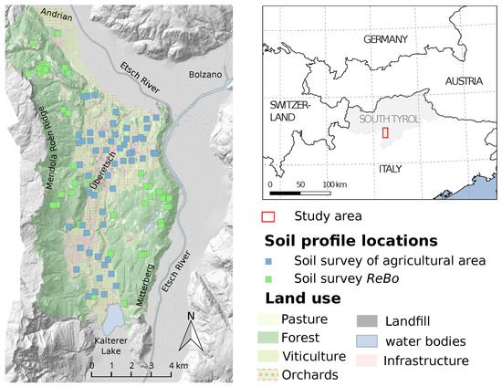
Figure 1.
Study area located in the Autonomous Province of South Tyrol (Bolzano), as indicated by the red rectangle. Digital terrain model and land use data were provided by the Autonomous Province Bolzano—South Tyrol.
The study area’s Alpine environment with its dynamic morphological history results in a wide range of soil parent materials, which paired with different types of former and current land use leads to a high diversity of soil types and soil features [10,38]. Cambisols and Fluvisols are characteristic of the paleovalley due to the fluviatile and glacial sediments, whereas Leptosols, Regosols and Umbrisols can be found on the steep calcareous slopes and siliceous outcrops. The soil data used in the study is part of two studies, focusing on forest and agricultural soils, respectively. The field work for the study which yielded the soil profile sites in the forest area of the study area as well as on the debris fan of Andrian, was performed in 2014 and 2015 under the premise of the project ReBo—Terrain Classification of ALS Data to support Digital Soil Mapping. The second soil survey was performed by [39] as an investigation of the agricultural areas in the Oltradige/Überetsch. The soil pits belonging to this study are all located on vineyards and apple orchards, and their positions, as well as those of the ReBo soil profiles, can be seen in Figure 1. Table 1 presents some descriptive statistics of the soil properties obtained from the field surveys, as well as sum parameters calculated by the SEPP tool for the soil profiles.

Table 1.
Descriptive statistics of the data from the field surveys as well as sum parameters calculated within the SEPP tool which are used as input data for calculating soil function fulfillment levels. For the statistics describing the A and B-horizons, from each soil profile the respective horizon (if present) with the greatest thickness was used for calculation.
The digital terrain model used in this study is provided at the homepage of the Autonomous Province of Bolzano-South Tyrol [40] or per email request (for the entire data set) and is the result of an airborne laser scanning mission performed in 2004 and 2005. The average last-pulse point density reported by [41] is 1.3 pts/m for the valley bottom and 0.8 pts/m for less densely inhabited areas and mountain slopes. The grid cell size is 2.5 m with an average standard deviation of heights reported as 6.7 cm. Computations on the the DTM were performed with the open source geographic information system GRASS GIS [42], for instance resampling to grid cell sizes of 10 and 50 m for considering scale when computing terrain parameters was performed with the implemented tool r.resamp.stats using average aggregation.
2.2. General Work-Flow
The general work-flow of the presented study can be separated into four different steps. In a first step the relevant soil information is entered into the SEPP tool, which then calculates a level of fulfillment for each soil function and soil pit. In a second step, a number of predictor variables, specifically local terrain parameters and landform classes, are derived from the digital terrain model for each of the soil pit locations. The third step is the statistical learning procedure, which includes feature selection and model validation. Forward step-wise feature selection based on maximizing cross-validated model accuracy is performed by first choosing the single predictor from the entire predictor variable set which on its own leads to the best model accuracy. Further variables are later added if they improve the model performance, which is assessed via cross-validation. In the last step, the modeling results are further investigated statistically and visually. This is done by analyzing the terrain parameter distribution of soil pits grouped with regard to their level of fulfillment for the different soil functions, and by predicting the fulfillment levels for each grid cell of the study area.
2.2.1. SEPP: Soil Evaluation for Planning Procedures
The software SEPP currently computes a soil function assessment based on soil pit descriptions. It requires that the pit descriptions are performed following the Austrian Soil classification [43,44], which is a morphological-genetic classification system closely related to the German classification [45]. The minimum soil profile site characteristics are local slope, altitudinal zone, thickness of organic horizons, humus form, soil depth, groundwater table, soil parent material, soil type, moisture level and land use. For each horizon, the minimum characteristics necessary for computing the levels of soil function fulfillment are the master horizon designation, depth, pH, proportion of the dominant soil structure type and class membership with regard to carbonate content, soil texture, coarse fragments content, organic content, bulk density, and soil structure. These class attributes can be substituted by exact lab values if available.
More complex horizon parameters, such as field capacity or cation exchange capacity, are approximated per m2 soil horizon using simple pedotransfer functions based on the aforementioned soil horizon characteristics (Table 2).These complex parameters are then summed up over the entire soil profile based on horizon thickness, often leading to units which refer to soil volume. These sum parameters are an essential part of the input parameters for calculating the levels of soil function fulfillment (Table 3). The 14 soil functions considered by SEPP can be classified into habitat for living organisms (specifically the sub-functions as habitat for drought-tolerant species, moisture-tolerant species, soil organisms or crops), infiltration and drainage regulation, groundwater recharge, nutrient provision, and filter and buffer for pollutants (with regard to the four subsets heavy metals, organic, acidifying and water-soluble contaminants), and are individually described below. The result of the soil function assessment is an an ordinal level between 1 and 5 for each soil function, with 1 signifying high fulfillment of this function, whereas 5 indicates low fulfillment.
Table 2.
Overview of the soil parameters parameters (rows) which are used in pedotransfer functions to compute the complex parameters per soil horizon (columns).
Table 3.
Overview of the soil parameters and soil profile sum parameters (rows) which are used as input for calculating the fulfillment levels of the different soil functions (columns).
Habitat for Drought-Tolerant Species
The levels of fulfillment for this soil function and the following one as a habitat for moisture-tolerant species are both assessed based on modifications of the approaches described by [46,47]. The evaluation of the extent to which a soil fulfills its function as a habitat for drought-tolerant species is based on the parameters land use, soil type and available field capacity. While the first two parameters are applied to distinguish especially suited (ruderal locations and corresponding soil types) or unsuited sites (mire deposits and soil types commonly linked to high water content), available field capacity is used to grade those soil profile sites representing the remaining land use and soil type combinations.
Habitat for Moisture-Tolerant Species
This function is evaluated similarly to the one for drought-tolerant species, in that specific soil types, e.g., Gleysols, are attributed specific soil function fulfillment levels. In addition, the depth of the groundwater table is used to distinguish sites with high levels of fulfillment, and the available field capacity is used to differentiate even further.
Habitat for Soil Organisms
The assessment of this soil function is done according to [48] with some minor adaptations. In this framework, a number of species groups are used as indicators for the composition of soil life, with emphasis on earth worms (Lumbricidae) as they are influential on soil structure and bioturbation. This method is based on the relationship between soil organism communities and a number of abiotic soil parameters. Specifically, one of 14 possible soil organism communities, which are the basis for the soil function fulfillment level, is attributed to a site according to a classification tree based on the parameters soil pH, moisture level, land use, and soil texture.
Habitat for Crops
The assessment of the extent to which a soil fulfills its function as a habitat for crops (excluding forestry) is performed according to the method proposed in the framework TUSEC-IP [47] by an accumulative rating of five criteria. The criteria general conditions of the profile site is rated based on soil depth, topsoil aggregate structure and the bulk density of topsoil and subsoil. While the criteria water supply is based on available field capacity and the depth of the groundwater table, the grade for air supply is derived from air capacity, and for nutrient supply the alkaline cation exchange capacity is regarded. The climate criteria is derived from the mean annual temperature of the growing season if available, or else replaced by proxy values such as mean annual temperature or altitudinal zone. The combination of the grades of the individual criteria leads to an overall level of fulfillment that is then adjusted for the slope gradient of the location.
Retention of Precipitation
This soil function is assessed using two different approaches, both of which are presented in this study. Following a modified version of the procedures presented by [46,49], the permeability coefficient (using either the average value of the soil profile or the minimum value) is combined with the water storage capacity. For more or less planar areas, the water storage capacity is regarded as the sum of the usable field capacity and the air capacity, whereas for steeper slopes only the former parameter is used. Additionally, permeability coefficient and water storage capacity are considered only for soil horizons not linked to groundwater or stagnant water.
Short-Term Retention of Heavy Precipitation
This soil function is assessed by applying a modified version of the scheme proposed by [47]. It differs from the previously mentioned precipitation retention, which considers long-lasting precipitation, by being based on the assumption that flooding hazards are greatest when soils are already saturated with water. Therefore only the air storage capacity is considered for the assessment. This retention volume is then compared to the design rainfall event under consideration of the infiltration rate.
Groundwater Recharge
Also following [47], the level of fulfillment for this soil function is evaluated using the same parameters as for precipitation retention, but under consideration of the assumption that very quick infiltration leads to an increase of pollutants in the groundwater. Following to the same reasoning, soil types linked to groundwater or locations with high groundwater table are given poorer fulfillment levels.
Nutrient Provision to Plants
Adhering to [50], the assessment of this soil function uses the parameter alkaline cation exchange capacity. As this is only a coarse approximation, this soil function is not differentiated into five, but only three classes (poor, average and high).
Carbon Storage
By applying a modified version of the rating proposed by [51], selected land uses, especially forests, are awarded high levels of fulfillment, whereas the remaining land uses are assessed based on the amount of organic matter, summed up over all soil horizons.
Retention of Heavy Metals
In this assessment, the ability to bind cadmium is used as a proxy for other heavy metals. Based on modifications of the procedures proposed by [46,52], in a first step this ability is evaluated for different pH for sandy soils with little organic content. The result is later adjusted with regard to organic matter content and soil texture as a proxy for clay content.
Transformation of Organic Contaminants
As organic pollutants are generally transformed by soil organisms, this soil function can be essentially assessed by rating the habitat conditions for soil micro-organisms. Consequently, the parameters which contribute to the rating procedure based on [49] are topsoil organic matter content, topsoil clay content and the average topsoil pH. In a first step, microbial activity is estimated based on humus form and pH, and then the level of soil function fulfillment is further differentiated based on organic matter and clay content.
Filtration and Buffering of Organic Contaminants
The evaluation of a representative contaminant (such as cadmium for heavy metals) is not feasible for organic contaminants due to their diversity. Therefore this soil function is assessed according to [50] by estimating a mean binding capacity for organic pollutants using organic matter and clay content for the fine material contained within a soil profile.
Retention of Water-Soluble Contaminants
For assigning a fulfillment level regarding the soil function of retaining water-soluble pollutants with emphasis on nitrate, the yearly seepage rate is calculated based on mean precipitation, mean evaporation and an estimate of surface run-off derived from soil texture. The fulfillment level is awarded based on the annual exchange rate of soil water by comparing seepage volume with field capacity [46].
Buffering of Acidic Substances
The potential buffer capacity is evaluated according to [46] by considering the alkaline cation exchange capacity and the carbonate content of the mineral horizons. Additionally, the buffer capacity of the organic layer is estimated from its thickness and the humus form.
2.2.2. The Predictor Variable Set: Terrain Parameters and Landform Classification
While a wide variety of different terrain parameters are available, the presented study concentrates on simple local terrain parameters as well as an automated landform classification algorithm. Regarding local terrain parameters, slope and a variety of curvature measures (planar, profile, cross-sectional, longitudinal, and tangential) were computed at varying window sizes and DTM resolutions using the GRASS GIS 7 [42] module r.param.scale. With regard to landforms, [24] showed in their comparison of automated landform classifications and the topographic description of soil pit sites, that the r.geomorphon algorithm by [53] is a valuable tool for use in soil survey and modelling. It uses pattern recognition based on line-of-sight calculations to classify each grid cell of a digital terrain model as one of 10 possible landforms (Figure 2).
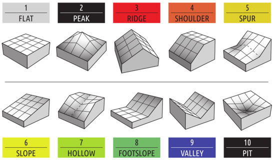
Figure 2.
The r.geomorphon algorithm classifies every grid cell of a given digital terrain model as one of these 10 landforms based on line-of-sight calculations (figure based on [53]).
These landform classifications were performed considering modifications of the two parameters search window size and flatness threshold. While the former parameter is responsible for how many surrounding grid cells are considered when performing the line-of-sight calculations, thus influencing the scale at which the landforms are computed, the latter represents the slope angles up to which a grid cell is regarded to be flat. In their analysis of different landform classifications, [24] demonstrated that investigating the result of varying flatness thresholds is of importance especially in an Alpine environment. In this study, terrain parameter derivation and landform classification were performed on the DTM of the entire study area, and then the specific terrain parameter values or landform classes of the soil pit locations were extracted and linked to the SEPP output to create the data set for modeling. Figure 3 shows three examples of maps of automated landforms and terrain attributes which were used as explanatory variables in this study.
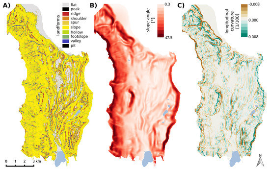
Figure 3.
Three exemplary terrain parameters and landform maps used in the study. (A) Landforms calculated with r.geomorphon at a grid cell size of 10 m, search radius of 100 m and flatness threshold of 4. (B) Slope at a grid cell size of 50 m and a search window of seven cells. (C) Longitudinal curvature at a grid cell size 10 m and a search window of 15 cells.
2.2.3. Statistical Learning and Variable Selection Procedure
Support vector machine (SVM) classification is a statistical learning approach first described by [54]. Its classification algorithm computes a hyperplane that best separates different classes by concentrating on certain data points of both classes, called support vectors, which are within a certain margin of the hyperplane. In this process, SVM classification also allows some points to be on the wrong side of the hyperplane, a behavior that can be addressed with a tuning parameter. By applying a radial kernel this linear binary classification can be extended to the non-linear case. A majority vote system then further allows the application of SVM classification for multiple classes. In the presented study, the SVM algorithm as implemented in the package e1071 [55] of the open source statistical computing environment R [56] was used.
A forward step-wise feature selection procedure based on cross-validation using SVM classification was applied to select the best parameter or parameter combination for each soil function. Cross-validation (five-fold) was also applied to the entire feature selection procedure. After partitioning the data set into five sets, one part was therefore set aside for validation, to be used after the entire feature selection procedure has been carried out with the four remaining parts. The usefulness of additional parameters in the model were evaluated using the one-standard-error-rule [57], meaning that the number of explanatory variables was seen sufficient if the improvement due to adding more explanatory variables did not exceed one standard error of the prediction accuracy. The selection process revealed that sometimes a number of parameter combinations led to comparable cross-validated accuracies, and that repetitions of the procedure showed a certain variation in these accuracy values. Therefore, the different parameter combinations were then compared by performing the 10-fold cross-validation 100 times, each time with 10 different, random partitions. The median values and distribution of accuracy values were compared, as well as the confusion matrices of the final modeled levels of soil function fulfillment (using the majority vote of the 100 predictions). Additionally, the models resulting from different parameter combinations were used to predict the soil function fulfillment levels for the entire study area and visualized as maps to examine how they performed spatially.
2.2.4. Post-Feature-Selection Analysis
After the feature selection procedure, the classes, consisting of soil pits with the same level of fulfillment for a given soil function, were analyzed with regard to the chosen terrain parameters or landform classification. This was performed with the original classes, but also with the predicted classes in order to investigate the effect of the different parameters on the output of the model based on the support vector machine classification. An example of such a box plot analysis of the distribution of terrain parameters is given in Figure 7. This analysis also gives insight into certain aspects with regard to user’s and producer’s reliability, which are accuracy measures derived from the confusion matrix based on the 100 prediction runs. User’s accuracy gives the percentage of correctly classified members of a class with regard to the total number of members in the respective reference class, which in this study is the classification performed by the SEPP tool. Producer’s reliability on the other hand relates the correctly classified members of a given class to the total number of members predicted by the model. If a landform classification rather than a local terrain parameter was chosen as best suited to distinguish between soil profile site locations with different fulfillment levels for a soil function, bar plots instead of box plots were applied to investigate and visualize the model output. For each soil function fulfillment level, the distribution of the 10 landforms was plotted in order to analyze how the dominance of different landforms changes for the different levels. These plots also demonstrate how the SVM model attributes the predicted levels to different landforms. Figure 8 shows such a plot for the soil function of transforming organic contaminants.
3. Results
The level of fulfillment for each of the 14 soil functions was calculated for each of the 108 soil profile pits in the study area with the SEPP application. Figure 4 shows the distribution of the fulfillment levels for each soil function as computed by the SEPP tool, whereas Figure 5 presents the predicted distributions based on SVM classification. Table 4 gives a overview of the feature selection and validation results, presenting the terrain parameters which were selected for modeling the levels of soil function fulfillment. In many cases, these parameter combinations consisted only of local terrain parameters, but sometimes a local terrain parameter was complemented with landform classes. In addition to the median cross-validated accuracy of 100 model runs, the test accuracy which results from using the same data for model fitting and validation is provided in Table 4.
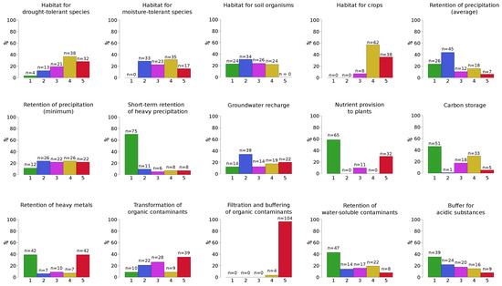
Figure 4.
Barplots representing the distribution of the soil function fulfillment levels of the locations of the 108 soil profiles assessed with the SEPP tool.
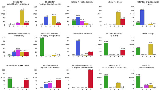
Figure 5.
Barplots representing the distribution of the soil function fulfillment levels of the 108 soil profiles as predicted by a SVM classifer based on the selected features presented in Table 4.
Table 4.
Results of the feature selection and validation. RES = resolution [m] of the applied digital terrain model, WS = window size [m] of computational algorithm, MCVA = median cross-validated accuracy of 100 model runs, TA = test accuracy (all profile sites are used as model and validation data).
Often two, or even just one, parameters are sufficient, as there is no increase in cross-validated prediction accuracy by adding more predictors. This can be observed in Table 5, which compares the accuracies from Table 4 to those achieved with SVM classifiers using an increased number of predictor variables. This larger set consists of all unique predictor variables which appeared in the entire five-fold cross-validation of a feature selection procedure which chooses 10 predictors per selection run. This amounts to 25–30 variables per model.
Table 5.
Comparison of the evaluation of models using only the features resulting from the feature selection procedure, and models implementing a larger predictor variable set. MCVA = median cross-validated accuracy of 100 model runs, TA = test accuracy (all profile sites are used as model and validation data).
3.1. Habitat for Drought-Tolerant Species
Figure 4 shows that of the 108 soil profile sites in the study area, 38 fall into fulfillment level class 4 and 32 into class 5 regarding the soil function of habitat for drought-tolerant species. The intermediate class 3 contains 21 soil profiles whereas the classes with high fulfillment levels (1 and 2) are attributed to only 4 and 13 sites, respectively. As the predictor set neither contains land use nor soil type, the SVM classification essentially attempts to model the different classes of available field capacity. In the majority of the feature selection runs a landform map based on a flatness threshold between 3 and 5, a spatial resolution of 10 m, and a search radius of 100 m was chosen as the first predictive feature. The landform flat is dominant amongst the profile sites with the lowest level of soil function fulfillment, which is accordingly connected to minimal curvature values around 0. The landform slope is most common for profiles at level 4, whereas spurs and hollows can present profile locations at fulfillment level 2 and, as expected, have increasingly negative minimum curvature values. A support vector classifier using these landforms and slope at a low DTM resolution as predictor variables results in a median cross-validated prediction accuracy of 50%, where the most common error is that a large number of sites are mistakenly classified as having fulfillment level 4. Nevertheless, the general implications of the feature selection are plausible, as flat areas can be expected to have higher field capacity values than sloping regions with negative curvature values.
3.2. Habitat for Moisture-Tolerant Species
None of the soil profile sites in the study area is awarded the best level of fulfillment (1) for its function as a habitat for moisture-tolerant species. As seen in Figure 4, the intermediate fulfillment level classes (2-4) are quite evenly distributed with 33, 23 and 35 members, respectively. The class with the lowest level consists of 17 soil profile sites. The soil parameters and profile site characteristics used for the evaluation of this soil function are similar to those used for the function as a habitat for drought-tolerant species. Consequently, a very similar landform classification is chosen in the feature selection procedure (Table 4), the only difference being a slightly tighter search window of 70 m. This feature is complemented by the local terrain parameter longitudinal curvature to achieve the best median cross-validated accuracy of 53.7%. The model predictions show that while the SVM classifier associates high levels of fulfillment with curvature values around zero, soil pits with the lowest level can be found at locations with negative longitudinal curvature. This trend is also visible in the landform distribution, were the landform flat, and, to a lesser degree, footslopes are characteristic for soil pits which fulfill the function as a habitat for moisture-tolerant species to a high degree. This combinations seems reasonable, given the potential hydrological situation in these positions.
3.3. Habitat for Soil Organisms
With the exception of the lowest soil fulfillment level class (5), which does not occur, the four other levels are distributed relatively evenly amongst the soil pits in the study area. Figure 6A shows the spatial distribution of the profiles sites and their soil function fulfillment levels in the study area. The class with the rather high level of 2 is the most common with 34 members. The feature selection procedure distinguished three local terrain parameters as being most useful in separating the soil profile sites with different fulfillment levels, specifically representatives of the parameters slope, convexity, and cross-sectional curvature. Lower convexity values characterize those soil profile sites best suited for soil organisms. Similarly, high slope values are helpful in separating members of the intermediate level (3) from the remaining three classes, based on the general trend that the two best levels are more closely associated with lower slope angles than the levels 3 and 4. An analysis of the cross-sectional curvature values shows that the class of soil profiles with level 4 tends to have more members related to slightly positive curvature values when compared to the other classes. A SVM classifier trained with the three aforementioned terrain parameters leads to a median accuracy rate of 59.3%, which is relatively high compared to other soil functions which also have profil sites belonging to more than three different fulfillment levels. Figure 6B shows how this prediction turns out spatially for the study area.
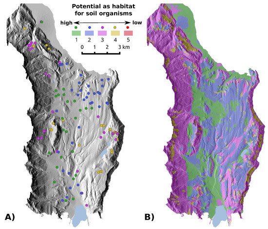
Figure 6.
(A) shows the study area along with the location of the soil profile sites and their level of soil function fulfillment regarding their function as a habitat for soil organisms as assessed by the SEPP tool. (B) shows the fullfillment levels as predicted by a SVM classifier based on the terrain parameters slope, convexity, and cross-sectional curvature.
3.4. Habitat for Crops
The soil pit locations within the study area exhibit a very low diversity with regards to the extent to which they fulfill the soil function as a habitat for crops. Only eight of the locations achieve the intermediate level 3, whereas the remaining soil pit sites are attributed with the poorer levels 4 (n = 62) and 5 (n = 38) by the SEPP tool. The feature selection procedure leads to a model which incorporates only the local terrain parameter slope based on the high resolution DTM and leads to a median cross-validated accuracy of 86%. The class of soil pits with fulfillment level 3 is not depicted in the model output, as the soil pits belonging to this class are misclassified as being part of the class with level 4, and, to a lesser degree, level 5.
Analysis of the distribution of the slope values of the different fulfillment levels based on the SEPP tool as well as predicted by a SVM classifier (Figure 7) shows that the SVM classifier applied a threshold of 15 to separate the locations with the levels 4 and 5, which is a direct result of this exact slope threshold applied by the algorithm in SEPP which calculates the fulfillment level of the soil function as a habitat for crops. The consequent difference in slope of these classes apparently overrules possible effects of other terrain parameters. This leads to the non-representation of the class with fulfillment level 3 in the model output. This issue is a consequence of the specifics of the study area, which can be roughly divided into the valley floors reserved for agriculture and the forested steep slopes. This is further complicated by the dominance of the classes with low function fulfillment levels, which cannot be solely attributed to the slope threshold, but also the generally rather shallow and skeleton-rich soils encountered.
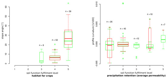
Figure 7.
Box plots representing the distribution of the slope angles and profile curvatures of the soil profile sites classified according to the levels of fulfillment of the functions as a habitat for crops, and precipitation retention, respectively. The green box plots represent the distribution of fulfillment levels as assessed by the SEPP tool, whereas the red box plots represent the distribution as predicted by a SVM classifier.
3.5. Retention of Precipitation
The fulfillment levels for the soil function of precipitation retention are relatively evenly distributed over the study area when calculated with minimum permeability, with only the best class having significantly less members than the other classes. However, when using average permeability coefficients the distribution shows a skew towards higher levels of fulfillment (Figure 4). Level 2 has the most members, constituting almost half of the soil profiles. The feature selection procedure for both calculation approaches shows that terrain parameters describing various forms of curvature are best suited to model the difference with regard to this soil function. Surprisingly, the specific curvatures differed for the two calculation methods.
For average precipitation retention, high resolution cross-sectional curvature was combined with profile curvature at medium (10 m) resolution to achieve a median cross-validated accuracy of 50.9%. The model output predicts four out of the five possible fulfillment level classes, with the intermediate level 3 missing. The predictions lead to an even larger dominance of level 2 than in the original data. While the 15 soil profile points with fulfillment level 1 which were attributed to level 2 by the SVM classifier seem acceptable, the 14 soil profiles with level 4 but classified as having level 2 are of more concern with regard to the predictive power of the model. The box plot analysis shows that for the model fitting, the SVM classifier concentrated on the outliers of the soil pits belonging to the classes with fulfillment levels 4 and 5 (Figure 7), which also leads to a low producer’s reliability for these classes.
For minimum precipitation retention, the best suited parameters were found to be high resolution planar curvature together with minimal curvature based on the low resolution DTM (50 m), i.e., a more regional scale topography. Combined by a SVM classifier, these predictor variables lead to a median cross-validated accuracy of just 41.6%. The confusion matrix shows misclassification between all classes, indicating that not only are the soil profiles distributed evenly amongst the different fulfillment levels, but this is also the case with regard to topography, leading to a low prediction accuracy.
3.6. Short-Term Retention of Heavy Precipitation
The capacity for short-term retention of heavy precipitation is assessed by SEPP as very high for 75 soil profiles in the study area, whereas the other fulfillment levels have relatively low membership numbers, distributed more or less evenly over the remaining classes. Feature selection identifies longitudinal curvature as helpful to separate the soil profiles with fulfillment level 4 from the rest of the profiles, as members of this class show higher, positive curvatures. This leads to a median accuracy of 73.1%, but also results in a large number of misclassifications to level 1 with only a limited number of soil profiles correctly attributed with fulfillment level 4. The other classes are not considered in the model output due to the dominance of level 1 on concave terrain and the assignment of convex areas such as ridges to fulfillment level 4.
3.7. Groundwater Recharge
The evaluation of the quantity and quality of groundwater recharge using the SEPP tool shows that almost 40% of the soil profiles exhibit the relatively high soil function fulfillment level 2, but also 41 profiles belong to the classes of soil profiles with levels 4 and 5. Accordingly, the SVM algorithm employs cross-sectional and profile curvature to generally divide the soil profiles into the classes 2, 4, and 5. This classification leads to a median cross-validated accuracy of 47.5%. Higher, and, in the majority, positive cross-sectional curvatures are attributed to soil profile classes with low function fulfillment levels. On the contrary, curvature values surrounding zero are linked to level 2, a class which incorporates a large proportion of soil profiles originally attributed with the levels 1 and 3 by the SEPP tool. While this sort of misclassification may seem acceptable when seeking a general trend with regard to the quality of groundwater recharge, the still substantial number of level 4 and 5 soils predicted to have level 2 by the SVM classifier indicates a strong influence of other factors beside topography.
3.8. Nutrient Provision to Plants
With regard to fulfilling the soil function of providing plant nutrients, 90% of the soil profiles belong to one of the extreme classes with level 1 or 5, whereas the intermediate level 3 has only 11 members. Compared to the predictive performance for other soil functions, this bimodal distribution leads to a relatively high cross-validated accuracy of 71.3% when using the local terrain parameter minimal curvature at a high DTM resolution of 2.5 m as the sole predictor variable. It is however important to consider that compared to other soil functions, the SEPP tool provides only three possible levels of fulfillment for this soil function. Due to the predominance of the more extreme levels, the model output predicts membership to one of these two soil profile classes, with the majority of the members of the intermediate class being attributed with fulfillment level 1. In this case, the classifier links the soil profiles with low fulfillment levels to negative minimal curvature values, while soils with higher levels are generally characterized by minimal values not far below zero.
3.9. Carbon Storage
Of the 108 soil profiles evaluated in the study area with the SEPP tool, 51 were assessed as having the highest level of fulfillment with regard to the function of soil as carbon storage. The class of soils with the second most members is that with fulfillment level 4, followed by the intermediate level 3. Almost the same local terrain parameter was chosen by the feature selection procedure as for the function of providing nutrients to plants, with minimal curvature leading to a prediction accuracy of 61.1%. When interpreting the model result, which only leads to two classes being predicted for the study area, representing the soil function fulfillment levels 1 and 4, it is important to acknowledge that the SVM classifier is essentially modeling forest land use for those profile sites with level 1. Consequently, areas with less distinct curvature, i.e., values surrounding zero, are classified as having lower fulfillment levels, whereas the sloping regions surrounding the paleovalley, which are in fact mostly covered by forest, are attributed a high fulfillment levels for carbon storage. The majority of the misclassifications are connected to level 4, which has a low producer’s reliability of 24%.
3.10. Retention of Heavy Metals
The distribution of the fulfillment levels for the soil function of retaining heavy metals can be characterized as bimodal. The more extreme levels 1 (high) and 5 (low) each have 42 members, whereas the remaining 24 profiles are distributed amongst the three intermediate classes, with level 3 being the largest class containing ten profile sites. For the model best suited to correctly predict fulfillment levels for as many soils as possible, a landform classification based on the 10 m DTM and a search window of 70 m surpassed the other predictor variables with a median classification accuracy of 63.9%. However, due to the dominance of two distinctly different classes over the remaining classes, the resulting model only predicts these two dominant fulfillment levels. Providing the model with further predictor variables did not improve the number of correctly predicted classes. In this model, the highest fulfillment level for the soil function of retaining heavy metals is linked to the landform flat, whereas all locations with a different automated landform class were attributed the lowest fulfillment level. The members of the three intermediate levels are almost equally divided among the dominant classes without a clear trend.
3.11. Transformation of Organic Contaminants
The class which represents the lowest function fulfillment level with regard to transforming organic contaminants is the most common with 39 member soil profiles. This class, which is characterized by low pH and/or low organic matter and clay content, can be predominantly found on ridges formed of rhyolite outcrops or steeper slopes. Accordingly, the feature selection procedure produces maximal curvature as an important terrain parameter and links soils with fulfillment level 5 to areas with higher, positive values of this parameter. Additionally, a landform classification based on a search window of 500 m, thus representing regional-scale topography, is implemented in the SVM classifier and identifies the landform slope as being closely correlated with a low fulfillment level for transforming organic contaminants. The landform class flat, on the other hand, is mainly linked to level 2, which is the class with the highest fulfillment level predicted by the SVM classifier (Figure 8).
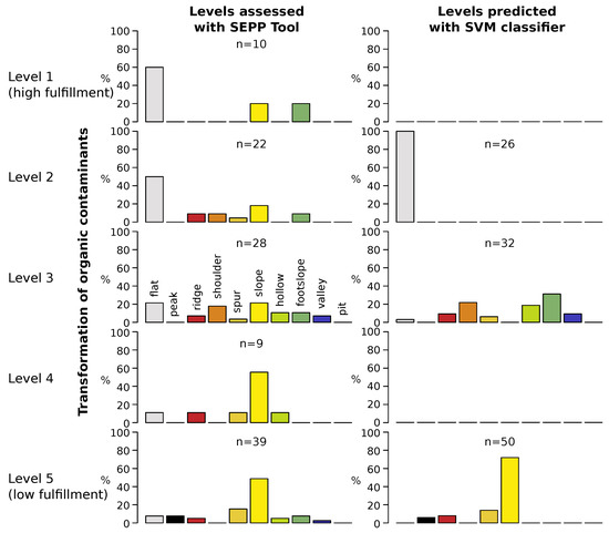
Figure 8.
Barplots representing the distribution of the landform classes for the different fulfillment levels regarding the soil function of transforming organic contaminants. The left column shows the distribution of the levels as evaluated by the SEPP tool, whereas the right column shows the distribution of the levels as predicted by the SVM classifier based on landforms and maximal curvature.
Together, a model fed with these two explanatory variables leads to a median cross-validated correct classification rate of 46.3%. It predicts the levels 2, 3, and 5, with the majority of class 1 soils being misclassified as level 3, and all but two of the level 4 soils incorporated into the class with fulfillment level 5.
3.12. Filtration and Buffering of Organic Contaminants
The distribution of the fulfillment levels of this soil function over the study area is very one-sided, with all but four soil profiles evaluated as belonging to the class with the lowest level. As a consequence, modeling the fulfillment levels of this soil function is not very productive, as the classifiers will simply classify the four soils with level 4 as level 5, which still leads to the high correct classification rate of 96%.
3.13. Retention of Water-Soluble Contaminants
The most dominant soil function fulfillment level with regard to retaining water-soluble contaminants such as nitrate is level 1 with 47 soil profiles. Levels 2 and 3 are similar with 14 and 17 members, followed by a slight peak in membership for level 4 with 22 profile sites. As the climatic framework is the same for the study area, this soil function is assessed in the SEPP tool based on only soil texture. A SVM classifier applying high resolution slope and minimum curvature as explanatory variables leads to a median cross-validated accuracy of 53.7%. Due to its dominance in the SEPP tool output, the predicted class with level 1, which the model links to very low slope angles and minimum curvature values not far away from zero, incorporates a large number of soil profiles with different levels. While this leads to a very high user’s accuracy of 96%, it is also responsible for a producer’s reliability of only 60%. The model predicts all classes except the one with fulfillment level 2, however levels 3 and 5 are projected for only two soils each, with level 3 producing a user’s accuracy of only 12%. The reason for this can be identified in the box plot analysis, which shows that for these 2 less populated classes the classifying algorithm concentrates on outliers in order to produce significant differences to the distribution of the relevant terrain parameters of the other classes.
3.14. Buffer for Acidic Substances
Soils with the highest level of fulfillment for this soil function are the most numerous in the study area, constituting 36% of all profile sites. With decreasing function fulfillment, the membership numbers also decrease, with only 9 soils attributed with the lowest level (5) by the SEPP tool. Planar curvature and slope, both computed with the high resolution (2.5 m) DTM and a local-scale window size of 12.5 m, result in a model with a median accuracy of 48.1%. A major drawback of this model is that with regard to the result based on the majority vote of 100 model runs, it fails to reproduce any members of the classes with level 2 and 5. While the small sample size may be an issue for level 5, 83% of the soils originally with level 2 are fitted into the predicted level 1, as these classes share a very similar terrain parameter distribution for both slope and curvature. Levels 3 and 4 are distinguishable by increasingly higher slope and also planar curvature values.
4. Discussion
The presented study shows that generally the levels of fulfillment of most soil functions can be linked to topography, however there are substantial differences with regard to the strength of this connections. As indicated in Table 4, the cross-validated accuracy of modeling soil function fulfillment varies from soil function to soil function, ranging from 41.6 to 86.1%. It must be kept in mind that the algorithms implemented in the SEPP tool are mostly expert knowledge-based and were not specifically intended for use in Alpine regions such as the study area. Furthermore, the study area has a long history of changing land use and a complex geologic setting, all of which have influence on the results of soil function assessments. In addition to the error which can be thereby be attributed to the non-inclusion of environmental covariates not directly derived from DTMs, such as parent material or local climate, a number of issues were encountered.
For one, topography, mainly represented by the terrain parameter slope, plays a role in some of the SEPP algorithms, depending on the soil function and also the specific fulfillment levels, which leads to high correct classification rates particularly for these classes. This influence of topography on the output of the SEPP tool can be either direct or indirect. An example for direct influence is the soil’s function as a habitat for crops. Originally, the assessment is based on a wide range of physical, chemical and biological soil parameters such as aggregate structure, bulk density, alkaline cation exchange capacity, organic matter, and others. However, the result is later directly adjusted based on a slope threshold of 15 degrees, as locations with steeper slopes are generally considered less suited for agricultural production (excluding pastures and forestry). This results in the highest classification accuracy of 86.1%, as the SVM classifier detects this threshold which leads to a model output that directly reflects this part of the evaluation procedure (Figure 7). This is also a consequence of the characteristics of the study area, which can be roughly divided into two topographically different regions: the valley floors reserved for agriculture and the forested steep slopes. Due to the generally rather shallow and skeleton-rich soils encountered, the classes with poor fulfillment levels (4 and 5) are dominant. This circumstance further boosts the above mentioned dualism, as slope turns out to be the main difference between fulfillment levels 4 and 5. The indirect implementation of the factor slope in the evaluation algorithm of the SEPP tool can be exemplified by the function of carbon storage, where soil profiles with the land use forest are immediately awarded the best fulfillment level. As mentioned in the results discussion of the function as a habitat for crops, forestry in the study area is more or less constrained to the steep slopes in the western part of the study area and the Mitterberg ridge which represents the eastern border. Consequently, curvature values which highlight non-flat areas but also strongly convex regions such as ridges, also characterize sites which are used for forestry rather than agriculture, thus constructing the link between curvature and the function of soil to store carbon. When considering the above mentioned direct and indirect implementations of slope, and the division of the study area based on slope and land use, it is necessary to keep in mind which other effects this may have. For instance, the less dominant influence of other topographic factors or landform classes on the calculation of function fulfillment levels may be overprinted by the effect of this slope threshold value or the link between slope and land use. Unfortunately, this cannot be mitigated by the addition of further terrain parameters to the model.
The analysis of the SVM classifier predicting the levels of function fulfillment for the average precipitation retention highlights the problem of outliers in the distribution (Figure 7). If the distributions of terrain parameters do not show obvious differences between the different levels, the classifier algorithm may revert to using outliers to characterize the different groups. Although these may indeed be values that best distinguish a certain subset of the data points and consequently lead to the best achievable correct classification rate, these values are unfortunately not representative of the data group in general. Nevertheless, such groupings may still result in valuable insights into some general trends in the data sets, even if they are exaggerated by the SVM classifier and lead to a small subset being overrepresented in the predicted fulfillment level membership. Another example for a soil function where certain groups in the model are in fact characterized by outliers is the function of retaining water-soluble contaminants.
An issue which is related to that of outliers can be found when investigating the model performance for soil functions which show a somewhat bimodal distribution with regard to their fulfillment levels as assessed with the SEPP tool. For instance, this is the case when comparing the distribution of the fulfillment levels of the soil function of providing nutrients to plants or the function of carbon storage in Figure 4 and Figure 5. The result is usually that this bimodality is reinforced in the SVM model, leading to the majority, if not all, of the soil profile sites being predicted as belonging to one of the two dominant classes and consequently limiting the number of fulfillment level classes in the model output. It is important to consider, especially for future research, that this bimodality, which can be found for a number of soil functions, may be linked to more dualistic characteristics of the study area, such as forest vs. agricultural land use, or silicate bedrock vs. limestone parent material, rather than topography.
Another aspect which necessitates discussion and is also related to the distribution of the fulfillment levels amongst the individual classes, is the question of sampling and, consequently, balanced classes. The advantage of a quite even distribution of the levels can be observed for the soil function as a habitat for soil organisms. This soil function shows a relatively high cross-validated accuracy, combined with a spatial prediction where all levels of fulfillment that are present in the SEPP output are also recreated in the model output (Figure 6), which is not the case for most other soil functions. While a sampling scheme which incorporates soil pits from all different levels of soil function fulfillment would be preferred, leading to a balanced data set, this is not always feasible, especially when relying on soil pit data from surveys focused on other soil aspects. If this is the case, the use of a smaller number of classes, as is done by the SEPP tool in the case of the function of providing nutrients for plants, may be more appropriate when searching for general trends with regard to the influence of topography on the evaluation of soil functions. This is also the case when a certain function shows only a limited number of levels in the specific study area. A different approach could be to quantify the severity of misclassifications when evaluating the prediction accuracy. As the fulfillment levels are in an ordinal scale, the difference in levels between the prediction and the actual level could be considered for weighted accuracies in future evaluations.
SVM classification was preferred to other statistical models, for instance logistic regression or random forests, for its smooth predictions [58] when applied as a spatial predictor. Additionally, SVM classification in the presented study is also used as an exploratory tool by applying a feature selection procedure to highlight those terrain parameters which are especially informative with regard to the fulfillment levels of a specific soil function. An issue encountered was that the accuracy values were found to be subject to variation when a classification was performed repeatedly with different random seeds. Using the median cross-validated correct classification rate was therefore deemed useful for evaluating the results of feature selection. Furthermore, other accuracy measures such as the kappa index are based on the assumption of simple random sampling [59] and not practicality, as is often the case especially in steep and forested regions where for instance access roads are essential. Additionaly, the use of the kappa index is not undisputed [60]. The analysis of the feature selection results has also shown that such a feature selection procedure is relevant also for SVM classification. To test this assumption, predictor variable sets consisting of up to 30 explanatory variables most frequently chosen in an expanded feature selection process were used to train SVM classifiers to model the fulfillment levels of the various soil functions (Table 5). While the test accuracy always increased with a larger predictor set, the median cross-validated accuracy, i.e., correct classification rate, was almost always lower than when using only the minimum set of explanatory variables as indicated by the feature selection procedure. This demonstrates that the issue of over-fitting should always be considered.
5. Conclusions
In this study, we presented the soil function assessment tool SEPP, and evaluated the extent to which local terrain parameters and landform classes can influence or recreate the level to which a soil fulfills certain soil functions. This was investigated by using support vector machine (SVM) classification and a feature selection procedure. For each of the 14 soil functions assessed by SEPP, the presented approach highlights those topographic attributes which are best suited for use as explanatory variables to model fulfillment levels. To a certain degree every soil function fulfillment level can be linked to different aspects of topography, but the accuracy with which a SVM classifier can predict them varied from function to function. The parameters slope and minimal curvature were the most frequently chosen terrain attributes, one or both being part of the explanatory variables for 8 of the evaluated soil functions. Landform classes constituted a part of the predictor variable set for three soil functions. The reasons for the wide range of cross-validated prediction accuracies are plentiful. For instance, the terrain parameter slope directly plays a role as a threshold in the evaluation algorithms of the SEPP tool for some soil functions, and indirectly through its influence on land use in the study area. This results in high prediction accuracies for the soil’s functions as a habitat for crops, and carbon storage, respectively. Another issue is that when the levels of function fulfillment as assessed with the SEPP tool were rather equally distributed amongst the soil profiles in the study area, this lead to all of these levels being predicted by the SVM classifier. An example for this is the soil’s function of habitat for soil organisms. However, when one or two fulfillment levels dominated the data set, this modal or bimodal distribution tends to be exaggerated in the predictive model at the cost of the fulfillment levels with less members. Furthermore, the plausibility of the results of such models should always be questioned under consideration of the possible influence by data outliers. The study also showed that feature selection procedures are of value also in SVM classification, especially when modeling is used as an exploratory data mining technique to increase understanding of underlying processes rather than simply predicting spatial distributions.
In the presented study, the regionalisation of point data was performed at the level of soil function fulfillment, however future research should also investigate the possibility of first predicting individual soil parameters and then performing the soil function assessment for each grid cell. Although the predictive power of models of soil function fulfillment based exclusively on terrain parameters is limited, the authors are of the opinion that the presented work is an important first step towards assessing the influence of topography on soil characteristics and, as a consequence, on the results of soil function assessments. By giving a first overview of the link between topography and the assessment of different soil functions, the study highlights those soil functions for which more detailed investigations into topographic influence are worthwhile. Additionally, the study shows that terrain parameters such as minimal curvature may be helpful as indicators of the degree to which soil functions are expected to be fulfilled by the soils in a given topographic setting.
Author Contributions
Conceptualization, F.E.G. and C.G.; methodology, F.E.G.; validation, F.E.G.and E.S.; formal analysis, F.E.G.; investigation, F.E.G. and J.B.; resources, C.G.; writing—original draft preparation, F.E.G. and E.S.; writing—review and editing, F.E.G., E.S. and C.G.; visualization, F.E.G.; project administration, C.G.; funding acquisition, C.G.
Funding
This research was performed within the project ’Terrain Classification of ALS Data to support Digital Soil Mapping’, funded by the Autonomous Province Bolzano–South Tyrol (Grant nr. 15/40.3).
Acknowledgments
We would like to thank Hannes Kleindienst of GRID-IT, Innsbruck, who wrote the SEPP tool code, for his support and help. We would also like to thank the three anonymous reviewers for their constructive comments and suggestions, which improved the final version of this manuscript.
Conflicts of Interest
The authors declare no conflict of interest. The funders had no role in the design of the study; in the collection, analyses, or interpretation of data; in the writing of the manuscript, or in the decision to publish the results.
Abbreviations
The following abbreviations are used in this manuscript:
| CV | Cross-validation |
| DTM | Digital Terrain Model |
| SFA | Soil function assessment |
| SVM | Support Vector Machine |
References
- European Commission. Toward a Thematic Strategy for Soil Protection. COM/2002/0179 Final; Technical Report; European Commission: Brussels, Belgium, 2002. [Google Scholar]
- Soil Threats in Europe: Status, Methods, Drivers and Effects on Ecosystem Services; EUR 27607 EN; Technical Report; JRC: Tokyo, Japan, 2016.
- Karlen, D.L.; Mausbach, M.J.; Doran, J.W.; Cline, R.G.; Harris, R.F.; Schuman, G.E. Soil Quality: A Concept, Definition, and Framework for Evaluation (A Guest Editorial). Soil Sci. Soc. Am.J. 1997, 61, 4–10. [Google Scholar] [CrossRef]
- Ad-hoc-Arbeitsgruppe Boden. Methodenkatalog zur Bewertung natürlicher Bodenfunktionen, der Archivfunktion des Bodens, der Nutzfunktion “Rohstofflagerstätte” nach BBodSchG Sowie der Empfindlichkeit des Bodens GegenüBer Erosion und Verdichtung; Bundesanstalt für Geowissenschaften und Rohstoffe (BGR): Hannover, Germany, 2007. [Google Scholar]
- Haslmayr, H.P.; Geitner, C.; Sutor, G.; Knoll, A.; Baumgarten, A. Soil function evaluation in Austria—Development, concepts and examples. Geoderma 2016, 264, 379–387. [Google Scholar] [CrossRef]
- Greiner, L.; Keller, A.; Grêt-Regamey, A.; Papritz, A. Soil function assessment: review of methods for quantifying the contributions of soils to ecosystem services. Land Use Policy 2017, 69, 224–237. [Google Scholar] [CrossRef]
- Blum, W.E.H. Functions of Soil for Society and the Environment. Rev. Environ. Sci. Biol. Technol. 2005, 4, 75–79. [Google Scholar] [CrossRef]
- Jenny, R.; Geitner, C.; Gruban, W.; Tusch, M. Soil Evaluation in Spatial Planning. A Contribution to Sustainable Spatial Development—Results of the EU-Interreg IIIB Alpine Space Project TUSEC-IP; Technical Report; Karo Druck KG/Sas: Frangart, Italy, 2006. [Google Scholar]
- Volchko, Y.; Norrman, J.; Rosén, L.; Bergknut, M.; Josefsson, S.; Söderqvist, T.; Norberg, T.; Wiberg, K.; Tysklind, M. Using soil function evaluation in multi-criteria decision analysis for sustainability appraisal of remediation alternatives. Sci. Total Environ. 2014, 485, 785–791. [Google Scholar] [CrossRef] [PubMed]
- Geitner, C.; Baruck, J.; Freppaz, M.; Godone, D.; Grashey-Jansen, S.; Gruber, F.E.; Heinrich, K.; Papritz, A.; Simon, A.; Stanchi, S.; et al. Chapter 8—Soil and Land Use in the Alps—Challenges and Examples of Soil-Survey and Soil-Data Use to Support Sustainable Development. In Soil Mapping and Process Modeling for Sustainable Land Use Management; Pereira, P., Brevik, E.C., Muñoz-Rojas, M., Miller, B.A., Eds.; Elsevier: Amsterdam, The Netherlands, 2017; pp. 221–292. [Google Scholar]
- Drobnik, T.; Greiner, L.; Keller, A.; Grêt-Regamey, A. Soil quality indicators—From soil functions to ecosystem services. Ecol. Indic. 2018, 94, 151–169. [Google Scholar] [CrossRef]
- Greiner, L.; Nussbaum, M.; Papritz, A.; Zimmermann, S.; Gubler, A.; Grêt-Regamey, A.; Keller, A. Uncertainty indication in soil function maps–transparent and easy-to-use information to support sustainable use of soil resources. SOIL 2018, 4, 123–139. [Google Scholar] [CrossRef]
- Dominati, E.; Patterson, M.; Mackay, A. A framework for classifying and quantifying the natural capital and ecosystem services of soils. Ecol. Econ. 2010, 69, 1858–1868. [Google Scholar] [CrossRef]
- Adhikari, K.; Hartemink, A.E. Linking soils to ecosystem services—A global review. Geoderma 2016, 262, 101–111. [Google Scholar] [CrossRef]
- Baveye, P.C.; Baveye, J.; Gowdy, J. Soil “Ecosystem” Services and Natural Capital: Critical Appraisal of Research on Uncertain Ground. Front. Environ. Sci. 2016, 4, 41. [Google Scholar] [CrossRef]
- Lagacherie, P.; McBratney, A. Chapter 1 Spatial Soil Information Systems and Spatial Soil Inference Systems: Perspectives for Digital Soil Mapping. In Digital Soil Mapping; Soil Science; Lagacherie, P., McBratney, A., Voltz, M., Eds.; Elsevier: Amsterdam, The Netherlands, 2006; Volume 31, pp. 3–22. [Google Scholar] [CrossRef]
- Herbst, P.; Gross, J.; Meer, U.; Mosimann, T. Geomorphographic terrain classification for predicting forest soil properties in Northwestern Switzerland. Z. Geomorphol. 2012, 56, 1–22. [Google Scholar] [CrossRef]
- Häring, T.; Dietz, E.; Osenstetter, S.; Koschitzki, T.; Schröder, B. Spatial disaggregation of complex soil map units: A decision-tree based approach in Bavarian forest soils. Geoderma 2012, 185, 37–47. [Google Scholar] [CrossRef]
- Ballabio, C. Spatial prediction of soil properties in temperate mountain regions using support vector regression. Geoderma 2009, 151, 338–350. [Google Scholar] [CrossRef]
- Gallant, J.C.; Wilson, J.P. Terrain Analysis-Principles and Applications; Chapter Primary Topographic Attributes; John Wiley & Sons, Inc.: Hoboken, NJ, USA, 2000; pp. 51–85. [Google Scholar]
- Olaya, V. Chapter 6: Basic Land-Surface Parameters. In Geomorphometry Concepts, Software, Applications; Developments in Soil Science; Hengl, T., Reuter, H.I., Eds.; Elsevier: Amsterdam, The Netherlands, 2009; Volume 33, pp. 141–169. [Google Scholar] [CrossRef]
- Kringer, K.; Tusch, M.; Geitner, C.; Rutzinger, M.; Wiegand, C.; Meissl, G. Geomorphometric Analyses of LiDAR Digital Terrain Models as Input for Digital Soil Mapping. Proc. Geomorph. 2009, 31, 74–81. [Google Scholar]
- Drăguţ, L.; Schauppenlehner, T.; Muhar, A.; Strobl, J.; Blaschke, T. Optimization of scale and parametrization for terrain segmentation: An application to soil-landscape modeling. Comput. Geosci. 2009, 35, 1875–1883. [Google Scholar] [CrossRef]
- Gruber, F.E.; Baruck, J.; Geitner, C. Algorithms vs. surveyors: A comparison of automated landform delineations and surveyed topographic positions from soil mapping in an Alpine environment. Geoderma 2017, 308, 9–25. [Google Scholar] [CrossRef]
- Behrens, T.; Scholten, T. Chapter 25 A Comparison of Data-Mining Techniques in Predictive Soil Mapping. In Digital Soil Mapping An Introductory Perspective; Developments in Soil Science; Elsevier: Amsterdam, The Netherlands, 2006; Volume 31, pp. 353–617. [Google Scholar] [CrossRef]
- Rossel, R.V.; Behrens, T. Using data mining to model and interpret soil diffuse reflectance spectra. Geoderma 2010, 158, 46–54. [Google Scholar] [CrossRef]
- Grimm, R.; Behrens, T.; Märker, M.; Elsenbeer, H. Soil organic carbon concentrations and stocks on Barro Colorado Island—Digital soil mapping using Random Forests analysis. Geoderma 2008, 146, 102–113. [Google Scholar] [CrossRef]
- Ließ, M.; Glaser, B.; Huwe, B. Making use of the World Reference Base diagnostic horizons for the systematic description of the soil continuum—Application to the tropical mountain soil-landscape of southern Ecuador. CATENA 2012, 97, 20–30. [Google Scholar] [CrossRef]
- Heung, B.; Bulmer, C.E.; Schmidt, M.G. Predictive soil parent material mapping at a regional-scale: A Random Forest approach. Geoderma 2014, 214, 141–154. [Google Scholar] [CrossRef]
- Ehsani, A.H.; Quiel, F. Geomorphometric feature analysis using morphometric parameterization and artificial neural networks. Geomorphology 2008, 99, 1–12. [Google Scholar] [CrossRef]
- Kempen, B.; Brus, D.J.; de Vries, F. Operationalizing digital soil mapping for nationwide updating of the 1:50,000 soil map of The Netherlands. Geoderma 2015, 241–242, 313–329. [Google Scholar] [CrossRef]
- Carré, F.; Girard, M. Quantitative mapping of soil types based on regression kriging of taxonomic distances with landform and land cover attributes. Geoderma 2002, 110, 241–263. [Google Scholar] [CrossRef]
- Dobos, E.; Hengl, T. Chapter 20 Soil Mapping Applications. In Geomorphometry Concepts, Software, Applications; Developments in Soil Science; Hengl, T., Reuter, H.I., Eds.; Elsevier: Amsterdam, The Netherlands, 2009; Volume 33, pp. 461–479. [Google Scholar] [CrossRef]
- McBratney, A.B.; Mendonca Santos, M.; Minasny, B. On digital soil mapping. Geoderma 2003, 117, 3–52. [Google Scholar] [CrossRef]
- Nussbaum, M.; Spiess, K.; Baltensweiler, A.; Grob, U.; Keller, A.; Greiner, L.; Schaepman, M.E.; Papritz, A. Evaluation of digital soil mapping approaches with large sets of environmental covariates. SOIL 2018, 4, 1–22. [Google Scholar] [CrossRef]
- Geitner, C.; Tusch, M. Soil Evaluation for Planning Procedures: Providing a Basis for Soil Protection in Alpine Regions; Borsdorf, A., Stötter, J., Veulliet, E., Eds.; Institut für Interdisziplinäre Gebirgsforschung: Hohe Tauern, Austria, 2008; Volume 2. [Google Scholar]
- Scholz, H.; Bestle, K.H.; Willerich, S. Quartärgeologische Untersuchungen im Überetsch. Geo Alp 2005, 2, 1–23. [Google Scholar]
- Baruck, J.; Nestroy, O.; Sartori, G.; Baize, D.; Traidl, R.; Vrščaj, B.; Bräm, E.; Gruber, F.E.; Heinrich, K.; Geitner, C. Soil classification and mapping in the Alps: The current state and future challenges. Geoderma 2016, 264, 312–331. [Google Scholar] [CrossRef]
- Thalheimer, M. Kartierung der landwirtschaftlich genutzten Böden des Überetsch in Südtirol (Italien). Laimburg J. 2006, 3, 135–177. [Google Scholar]
- Autonomous Province Bolzano—South Tyrol. Download Landeskartographie. Available online: http://www.provinz.bz.it/natur-umwelt/natur-raum/kartographie/download-und-webgis.asp (accessed on 4 March 2019).
- Wack, R.; Stelzl, H. Laser DTM Generation for South-Tyrol and 3D-Visualization. In Proceedings of the International Archives of Photogrammetry, Remote Sensing and Spatial Information Science, Vienna, Austria, 3–5 October 2005. [Google Scholar]
- GRASS Development Team. Geographic Resources Analysis Support System (GRASS GIS) Software, Version 7.0; Open Source Geospatial Foundation: Chicago, IL, USA, 2016. [Google Scholar]
- Nestroy, O.; Danneberg, O.; Englisch, M.; Geßl, A.; Hager, H.; Herzberger, E.; Kilian, W.; Nelhiebel, P.; Pecina, E.; Pehamberger, A.; et al. Systematische Gliederung der Böden Österreichischs (Österreichische Bodensystematik 2000). Mitt. Österr. Bodenkdl. Ges. 2000, 60, 327–355. [Google Scholar]
- Nestroy, O.; Aust, G.; Blum, W.; Englisch, M.; Hager, H.; Herzberger, E.; Kilian, W.; Nelhiebel, P.; et al. Systematische Gliederung der Böden Österreichs. Österreichische Bodensystematik 2000 in der revidierten Fassung von 2011. Mitt. Österr. Bodenkdl. Ges. 2011, 79, 1–98. [Google Scholar]
- Ad-hoc-Arbeitsgruppe Boden. Bodenkundliche Kartieranleitung KA5; Schweizerbart Science Publishers: Stuttgart, Germany, 2005. [Google Scholar]
- BayGLA and BayLfU. Das Schutzgut Boden in der Planung-Bewertung Natührlicher Bodenfunktionen und Umsetzung in Planungs-und Genehmigungsverfahren; Technical Report; Bayerisches Geologisches Landesamt, München und Bayerisches Landesamt für Umweltschutz: Augsburg, Germany, 2003. [Google Scholar]
- Lehmann, A.; David, S.; Stahr, K. TUSEC—Bilingual-Edition: Eine Methode zur Bewertung natürlicher und Anthropogener Böden (Deutsche Fassung) Technique for Soil Evaluation and Categorization for Natural and Anthropogenic Soils (English Version); Hohenheimer Bodenkundliche Hefte, Universität Hohenheim-Institut für Bodenkunde und Standortslehre: Hohenheim, Germany, 2008; Volume 86. [Google Scholar]
- Beylich, A.; Höper, H.; Ruf, A.; Wilke, B.M. Bewertung des Bodens als Lebensraum für Bodenorganismen im Rahmen von Planunsprozessen. Mitt. Deutsch. Bodenkund. Ges. 2005, 107, 183–184. [Google Scholar]
- Lehle, M.; Bley, J.; Mayer, E.; Veit-Meya, R.; Vogl, W. Bewertung von Böden Nach Ihrer Leistungsf ähigkeit; Luft, Boden, Abfall 31; Landesamt für Umwelt, Messungen und Naturschutz Baden-Würtemberg: Karlsruhe, Germany, 1995. [Google Scholar]
- Müller, U.; Waldeck, A. Auswertungsmethoden im Bodenschutz—Dokumentation zur Methode des Niedersächsischen Bodeinformationssystems (NIBIS); GeoBerichte 19, Landesamt für Bergbau, Energie und Geologie: Hannover, Germany, 2011. [Google Scholar]
- Gerstenberg, J.H.; Smettan, U. Erstellung von Karten zur Bewertung der Bodenfunktionen—Umsetzung der im Gutachten von Lahmeyer aufgeführten Verfahren in Flächendaten; Technical Report; Senatsverwaltung für Stadtentwicklung Berling: Berlin, Germany, 2005. [Google Scholar]
- AG Boden. Methodendokumentation Bodenkunde—Auswertungsmethoden zur Beurteilung der Empfindlichkeit und Belastbarkeit von Böden; Bundesanstalt für Geowissenschaften und Rohstoffe und Staatliche Geologische Dienste in der Bundesrepublik Deutschland: Stuttgart, Germany, 2000. [Google Scholar]
- Jasiewicz, J.; Stepinski, T.F. Geomorphons—A Pattern Recognition Approach to Classification and Mapping of Landforms. Geomorphology 2013, 182, 147–156. [Google Scholar] [CrossRef]
- Cortes, C.; Vapnik, V. Support-vector networks. Mach. Learn. 1995, 20, 273–297. [Google Scholar] [CrossRef]
- Meyer, D.; Dimitriadou, E.; Hornik, K.; Weingessel, A.; Leisch, F. e1071: Misc Functions of the Department of Statistics (e1071), TU Wien; R Package Version; Vienna University of Technology: Vienna, Austria, 2014. [Google Scholar]
- R Core Team. R: A Language and Environment for Statistical Computing; R Foundation for Statistical Computing: Vienna, Austria, 2014. [Google Scholar]
- James, G.; Witten, D.; Hastie, T.; Tibshirani, R. An Introduction to Statistical Learning; Springer: New York, NY, USA, 2013. [Google Scholar]
- Steger, S.; Brenning, A.; Bell, R.; Petschko, H.; Glade, T. Exploring discrepancies between quantitative validation results and the geomorphic plausibility of statistical landslide susceptibility maps. Geomorphology 2016, 262, 8–23. [Google Scholar] [CrossRef]
- Congalton, R.G. A review of assessing the accuracy of classification of remotely sensed data. Remote Sens. Environ. 1991, 37, 35–46. [Google Scholar] [CrossRef]
- Pontius, R.G.; Millones, M. Death to Kappa: birth of quantity disagreement and allocation disagreement for accuracy assessment. Int. J. Remote Sens. 2011, 32, 4407–4429. [Google Scholar] [CrossRef]
© 2019 by the authors. Licensee MDPI, Basel, Switzerland. This article is an open access article distributed under the terms and conditions of the Creative Commons Attribution (CC BY) license (http://creativecommons.org/licenses/by/4.0/).