Prescribed Fire Smoke: A Review of Composition, Measurement Methods, and Analysis

Abstract

Prescribed fire has become an increasingly important strategy for removing biomass from forests and mitigating the risk of severe wildfire. When considering where and to what extent prescribed fire should be applied, land resource managers must consider a host of concerns including biomass density, moisture content, and meteorological conditions. These variables will not only affect how effective the burn will be, but also what sort of smoke is produced by the prescribed fire and how that smoke impacts individuals and local communities. After briefly summarizing how prescribed fire practices have evolved, this review describes how the properties of prescribed fire smoke depend on prescribed fire conditions and the methods used to measure molecular and particulate species in prescribed fire smoke. The closing section of this review identifies areas where advances in smoke monitoring and characterization can continue to improve our understanding of prescribed fire behavior.

1. Introduction

Prescribed fire describes the intentional burning of vegetation to reduce fuel accumulation with the aim of reducing wildfire risk [1,2]. In this context, prescribed fires are set for a specified time in a designated area. Choosing where to use prescribed fire requires careful consideration of factors including environmental conditions, impacts on an ecology’s microbiome, and effects on wildlife and people. However, by creating firebreaks and reducing fuel loads near populated areas, prescribed fire creates landscape buffers, slowing or stopping the spread of unconstrained wildfires. Moreover, prescribed fire practices provide opportunities for fire professionals to practice fire management techniques in safe and supervised settings.

This review summarizes current knowledge about one consequence of prescribed fire, namely, prescribed fire smoke. Specifically, the review discusses prescribed fire smoke composition and the methods used to measure prescribed fire smoke’s molecular and particulate constituents. This review is intended to inform scientists and engineers about important issues related to prescribed fire smoke. More detailed assessments of measurement technologies can be found elsewhere in the literature and are referenced in the appropriate sections below. After highlighting similarities and differences between smoke from prescribed fire and wildfire, this review provides a brief history of how prescribed fire has evolved as a strategy for managing landscapes before examining prescribed fire smoke composition and how that composition is measured. The review concludes with a discussion of current challenges and opportunities for prescribed fire smoke research.

Prescribed fire plays a critical role in maintaining healthy ecosystems. Many plant species have evolved to thrive with periodic fires that clear out invasive plants, release nutrients back into the soil, and encourage the growth of native vegetation. In fire-adapted ecosystems, the absence of regular burning can lead to ecological imbalance and greater vulnerability to damaging wildfires [3]. In this way, prescribed fire provides long-term benefits by preventing the extensive destruction and ecological disruption caused by wildfires. Prescribed burning is therefore a controlled and deliberate act to safeguard ecosystems against more severe natural disturbances including intense wildfire.

Wildfire, in contrast, disrupts the environment and has resulted in extensive loss of properties and, in some cases, loss of lives. Wildfire can be caused either by natural events (e.g., lightning) or human activity and can become extremely destructive to ecosystems and communities if not suppressed. In 2021, the total loss accumulated from wildfire in Maui Hawaii was estimated to be about USD 5.5 billion [4]. Similarly, the adverse impacts from wildfires in Southern California in January 2025 will last for decades [5]. While wildfires may be caused naturally, wildfire’s intensification and destructive power can be blunted by strategically using prescribed fire proactively. Many forecasts predict increased wildfire occurrence in the coming years due to changes in climate conditions [4,6,7,8]. Wildfires often burn with such intensity that they consume nutrients required for sustainable regrowth. The heat and severity of wildfires can sterilize soil, destroy seed banks, and inhibit plant regeneration, making it difficult for both dominant and non-dominant species to recover [9,10]. Representative images of wildfires and prescribed fire are shown in Figure 1.

While prescribed fire and wildfire share some characteristics, they differ in important ways: prescribed fires are intended to burn with low intensity and have a restorative impact on an ecosystem’s flora and fauna. Differences in fire intensity are readily apparent in thermal imagery studies where prescribed fire radiative power (FRP) peaks at ~1000 W/m², but wildfire FRP can be as high as 5 × 10⁴ W/m² [12,13]. These differences have profound effects on a system’s ecology. Prescribed fire can temporarily improve the infiltration capacity and soil water content while increasing the stability of soil aggregates and total organic carbon in the upper soil layer. Bulk soil densities are also slightly decreased post-prescribed fire [14,15]. The intended long term consequence of prescribed fire is a sustainable, resilient ecosystem, whereas extreme wildfires will often cause irreversible harm to a landscape [16].

Differences in fire intensity are evident in the smoke and particulates generated by prescribed fire and wildfire. Smoke produced by prescribed fire and wildfire has both acute and chronic impacts on human health. Biomass burning results in a host of small-molecule species including carbon dioxide (CO₂), carbon monoxide (CO), nitrogen oxides (NO_x), and methane (CH₄), as well as larger molecules such as formaldehyde (CH₂O), ethylene (C₂H₄), benzene (C₆H₆), and higher-molecular-weight aromatics [17,18,19]. Particulate matter (PM) resulting from incomplete combustion and from aggregation in the atmosphere is also a dominant component of prescribed fire and wildfire smoke. Constituents in wildfire smoke are often more heterogeneous as wildfires can consume physical structures in addition to biomass. Wildfires often produce dense smoke containing high-density fine particulate matter, carbon monoxide, and other harmful species, leading to significant health concerns and environmental degradation [20,21,22,23,24]. Prescribed fires, managed with precision, produce less smoke and are timed to minimize impacts on air quality in nearby communities [25].

This review describes current knowledge about prescribed fire smoke composition and prescribed fire smoke characterization. The work is motivated by several considerations that are increasingly relevant as prescribed fire becomes a more common practice for wildland management throughout the United States. First, while considerable effort has focused on characterizing smoke from wildfires, the literature contains far fewer reports that quantify prescribed fire smoke. Second, most prescribed fire research performed in the United States has been carried out in the southeast part of the country, and findings may not be widely transferrable to locations where topography, biomass, and meteorological conditions vary substantively. We do not specifically include satellite methods as a means for evaluating prescribed fire smoke, as these methods are effective at tracking fire severity [26,27] and the spread of fire generated smoke [28] but have limited ability to predict fire smoke composition [29]. After first briefly reviewing the evolution of prescribed fire as a means of managing lands to reduce wildfire risk, we consider several important aspects of prescribed fire smoke and, whenever possible, compare findings for prescribed fire to those reported for wildfire. Specifically, we summarize the scientific community’s current understanding of (1) prescribed fire smoke composition and (2) measurement and monitoring methods. The review closes with a description of current practices for measuring and tracking smoke from prescribed fires and identifies needs for improved prescribed fire smoke characterization.

2. Prescribed Fire—An Evolving Strategy for Land Management

Using prescribed fire to manage landscapes is not a new idea. Indigenous populations have deployed fire to prepare land for agriculture and restore ecosystem health for improved hunting for millenia [30,31]. With European expansion and reduced emphasis on sustainable landscape management, prescribed fire became less common. During the 19th and early 20th centuries logging for agriculture, fuel, and industry created large amounts of woody debris that fueled devastating wildfires. These fires led to the rise of fire suppression policies, including the USFS 10 AM Policy of 1935, and the establishment of federal land management agencies like the US Forest Service (1905) and National Park Service (1916). Advertising campaigns, such as Smokey Bear, reinforced fire prevention efforts [32,33,34,35].

Early fire control efforts were limited by infrastructure, but post-World War II advances, including road building and surplus military equipment, led to more effective suppression. The decline in both natural and indigenous burning also led to major changes in fire occurrence across landscapes [36]. In the eastern US, wildfire frequency dropped significantly, and in the western US, burned areas reached their lowest levels in the 1970s before increasing again. Canada saw rising fire activity from 1959 to the 1990s, followed by a decline, except in western provinces [37,38].

Despite recent media attention to catastrophic wildfires nationwide, modern fire occurrence remains far lower than historical levels. Studies estimate that in the conterminous US, about 10 times less land burned in the late 20th century compared to pre-industrial times [39]. Canadian boreal forests also burn at a rate five times lower than historically recorded [40]. Fire trends in Mexico and Central America vary. Only in the second half of the 20th century was prescribed fire once again viewed as an effective tool for maintaining healthy forests and reducing the risks of extreme wildfires [41,42].

Prescribed fire is practiced throughout the United States, primarily on public lands by the US Forest Service and other agencies. However, much of the research into prescribed fire behavior has been performed in the American Southeast. For example, a 5-year study performed on military bases in South and North Carolina used both field and laboratory measurements to characterize the smoke produced from 13 prescribed fires. Through extensive use of Fourier transform infrared (FTIR) spectroscopy and gas chromatography–mass spectrometry (GC-MS), researchers identified more than 200 trace gases and formulated exposure estimates for firefighters on the prescribed fire control lines [43]. More recently, researchers have developed computer algorithms to distinguish prescribed burns from wildfires using satellite data from the Southeastern United States acquired between 2013 and 2020 [44]. From satellite imagery and computer modeling, researchers generated three-dimensional prescribed burning emission maps to describe chemical transport. An extensive study focused on biomass emissions compared laboratory measurements using fuels commonly consumed in prescribed fires in the Southeastern US with both airborne and ground-based measurements from prescribed fires in North Carolina to better understand organic emissions and revealed that a sizable fraction of these emissions were not identifiable using conventional measurement methods [45].

In general, the public is often broadly supportive of using prescribed fire to mitigate the risks of potentially catastrophic wildfire. A poll conducted in 2022 sampled opinions from California communities impacted by either wildfire or prescribed fire smoke. The sample pool was weighted towards an older population (≥65 years old) and more than half of those people surveyed (58%) reported adverse health impacts from wildfire smoke while only 28% made the same self-assessment about smoke from prescribed fire smoke [46]. Other work reported that communities in fire-prone areas are well aware of factors affecting wildfire risk. A majority of people sampled in these communities supported using prescribed fire proactively to lower the risk of wildfire. In this context, survey respondents accepted temporary risks posed by prescribed fire smoke. In general, most people do not consider smoke as a significant barrier to the use of prescribed fire [47]. This attitude is reflected in the growing deployment of prescribed fire as a forest management tool. A 2023 report written jointly by the USFS and USDA [48] noted “that landscapes are in critical need of work to reduce exposure to and risk from wildfires. Hazardous fuels reduction is a major component of this work, and prescribed fire is key to reducing fuels.”

3. Smoke Composition—Prescribed Fire vs. Wildfire

Smoke from both prescribed fires and wildfires has been characterized extensively and shows clear differences. Prescribed fires are controlled, low-intensity burns conducted under carefully monitored conditions. Smoke generated by prescribed fires typically remains at lower altitudes, travels shorter distances, and poses fewer risks to public health. Wildfires, on the other hand, are uncontrolled, often high-intensity events caused by dry vegetation, wind, and heat. The smoke resulting from wildfires often rises to higher altitudes, dispersing pollutants over large areas and over long distances.

This section considers two contributions to smoke from prescribed fire and, when appropriate, wildfire: (1) chemical composition and (2) particulate matter (Figure 2).

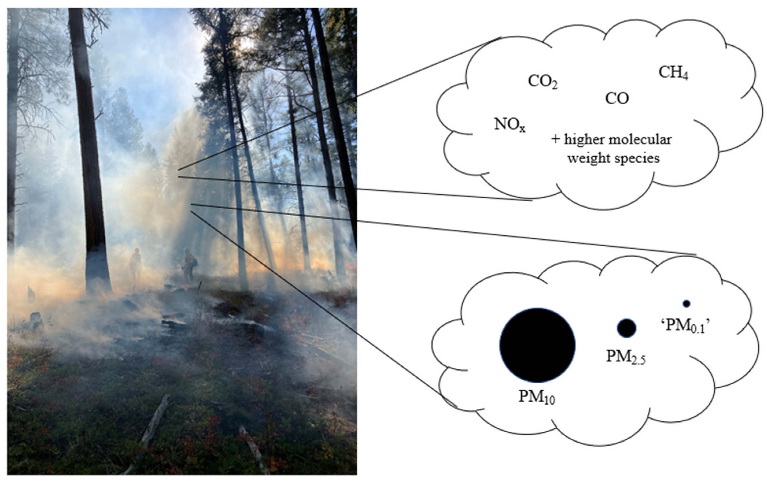
3.1. Chemical Composition

Chemical composition refers to the molecular species resulting from biomass burning. These species can be as small as molecular hydrogen (H₂) or as large as polyaromatic hydrocarbons. Most of these species have regulatory limits, and many are considered acutely toxic (e.g., HCN) or chronically toxic (e.g., benzene). Particulate matter, in contrast, is less well defined and describes the particulates formed from incomplete combustion. Particulate matter is classified by size, with PM₁₀ particulate matter consisting of particles having diameters ≤ 10 μm and PM_2.5 particulates having diameters ≤ 2.5 μm. PM_2.5 particles are considered to pose a greater threat to human health because these smaller particles transfer more easily across the alveolar boundary and into the bloodstream. The scientific and public health communities have considered creating a third class of particulates having even smaller diameters (PM_0.1 or particles having diameters ≤ 100 nm) because these ultrafine particles are believed to exacerbate asthma and an individual’s response to allergens as well as adversely impact cardiovascular and respiratory function [49].

Prescribed fire generates a wide range of species in its smoke, including inorganic molecules such as carbon monoxide (CO), carbon dioxide (CO₂), nitrogen oxides (NO_x), and ammonia (NH₃) as well as organic constituents such as methane (CH₄), ethylene (C₂H₄), methanol (CH₃OH), acetic acid (C₂H₄O), formic acid (CH₂O) and many more [50]. In a 2-year-long emission study carried out at a military installation in California, CO was one the few targeted species of the prescribed fire smoke. The CO was a tool in determining the emission ratio of the burn for several species including black and brown carbon which were found to be 0.014 μgm⁻³ ppb⁻¹ and 0.442 μgm⁻³ ppb⁻¹, respectively [51]. Nitrogen oxides (NO_x) have been found in a significant quantity in prescribed fire smoke. NO_x are important since they contribute to the formation of ozone and secondary pollutants like peroxyacetyl nitrate (PAN) that are known to adversely impact air quality and human health. Additionally, NO_x influences atmospheric chemistry by affecting the oxidation capacity in the atmosphere [52,53].

This section focuses on the behaviors of three of the most common carbon-containing species in prescribed fire smoke: CH₄, CO₂, and CO. In addition, the origins and impacts of NO_x and other nitrogen containing species found in prescribed fire smoke are also discussed.

CH₄ is an important indicator of the type of combustion in prescribed fires. Higher levels of CH₄ in smoke indicate the lack of enough oxygen and the combustion is therefore incomplete, implying a smoldering fire. Furthermore, the quantity of CH₄ present in smoke is often benchmarked against the amount of CO or CO₂ produced to assess fire temperature and the extent of biomass oxidation [54]. Often, more CH₄ will be produced by biomass having high moisture content. A study in Florida wetlands showed significantly increased methane (CH₄) emissions, with postfire fluxes exceeding 0.15 g CH₄ m⁻² d⁻¹ [55].

Two of the most common molecules used as diagnostics are CO₂ and CO. CO₂ is the most abundant gas produced in wildland fires, and while prescribed fire typically generates less CO₂ than wildfire due to the lower intensity of the burn, CO₂ production from prescribed fire remains significant. Incomplete combustion can also generate significant amounts of carbon monoxide (CO). CO₂ and CO concentrations are used to determine combustion efficiencies and modified combustion efficiencies. The relationship between the amounts of CO₂ and CO produced is described by a fire’s modified combustion efficiency (MCE). The MCE is an important parameter used to evaluate the completeness of combustion in wildland burning including both wildfires and prescribed fire:

$$\mathrm{M}\mathrm{C}\mathrm{E}={\displaystyle \frac{{[\mathrm{C}\mathrm{O}}_2]}{{[\mathrm{C}\mathrm{O}}_2]+[\mathrm{C}\mathrm{O}]}}$$

Different studies use different units for concentrations including grams, micrograms, or ppm, but the MCE itself is invariant to the source of the measurements. In the limit of complete combustion, the MCE converges to unity while lower intensity, smoldering fires will lead to MCE values closer to 0.8. MCE values for prescribed fires are generally less than 0.9 and closer to 0.8 due to prescribed fire’s low-intensity, smoldering nature [56,57]. MCE values are impacted by the types of fuel and the conditions under which they burn. For example, MCE values ranged 0.86 to 0.94 in field measurements from boreal fires in Boise, ID with smoldering smoke producing more methane than CO or CO₂ [58]. On the other hand, MCE values for Amazon tropical forest fires were around 0.94 producing more non-methane gases [59], suggesting a combination of smoldering and flaming combustion. A study conducted in August 2011 in the northern Rocky Mountains of the United States investigated emissions from three wildfires and one prescribed fire in mixed conifer forests during wildfire season [60]. Using airborne instrumentation, researchers measured combustion products and found that the average MCE was 0.883, indicating a relatively low combustion efficiency, particularly when compared to previous studies of prescribed fires.

Carbon budgets refer to the permissible amount of CO₂ emitted over a set period and are reported in terms of mass of carbon in tons emitted per unit area in hectares [61]. Consequently, carbon budgets are important to consider when deciding where and at what rate a prescribed burn is carried out. In addition to the amount of biomass being burned, a second factor that impacts carbon budgets is the biomass moisture content. One example of how moisture affects carbon budgets is a study examining CO₂ output from two prescribed fire events, one carried out in shrub savannas and one carried out in grassland [62]. Biomass in shrub savannas has low moisture content and burns with high intensity leading to increased CO₂ emission. In contrast, grassland fires using fuel with higher moisture content burns with lower intensity and will have a lower carbon budget. These two situations—shrub savanna and grassland prescribed fires—were recently compared and had carbon budgets of 1.61  ±  0.13 t C ha⁻¹ and 1.01  ±  0.13 t C ha⁻¹, respectively [62].

Carbon budgets are useful diagnostics but describe only one aspect of prescribed fire’s impact. Prescribed fire helps shape the global carbon cycle by both releasing carbon into the atmosphere (and determining a fire’s carbon budget) and creating pyrogenic carbon (PyC), a stable form of carbon produced through incomplete combustion. In Australian eucalyptus forests, researchers quantified PyC formation from low to moderate severity prescribed fires, and reported that ~23% of the carbon affected by fire was converted into PyC, while the remaining 77% was converted to smoke emission [63]. These data are important because PyC represents affected carbon that does not contribute to the carbon budget as CO₂ but does transform biomass carbon into a material that cannot contribute to landscape and ecosystem resilience. Usually, prescribed burns have higher impacts on carbon content from the forest floor and less impact on deadfall and trees [64].

A separate way of reporting smoke’s molecular composition is to use emission factors. Emission factors (EFs) represent the amount of a specific pollutant emitted per unit of fuel burned and can be applied to specific types of gases. A high EF indicates a higher release of smoke product per unit of fuel consumed while a lower EF indicates cleaner combustion with lower pollutant emissions. EFs are defined as follows:

$$\mathrm{E}\mathrm{m}\mathrm{i}\mathrm{s}\mathrm{s}\mathrm{i}\mathrm{o}\mathrm{n} \mathrm{F}\mathrm{a}\mathrm{c}\mathrm{t}\mathrm{o}\mathrm{r}={\displaystyle \frac{\mathrm{M}\mathrm{a}\mathrm{s}\mathrm{s} \mathrm{o}\mathrm{f} \mathrm{p}\mathrm{o}\mathrm{l}\mathrm{l}\mathrm{u}\mathrm{t}\mathrm{a}\mathrm{n}\mathrm{t} \mathrm{e}\mathrm{m}\mathrm{i}\mathrm{t}\mathrm{t}\mathrm{e}\mathrm{d} \left(\mathrm{g}\right)}{\mathrm{M}\mathrm{a}\mathrm{s}\mathrm{s} \mathrm{o}\mathrm{f} \mathrm{f}\mathrm{u}\mathrm{e}\mathrm{l} \mathrm{b}\mathrm{u}\mathrm{r}\mathrm{n}\mathrm{e}\mathrm{d} \left(\mathrm{k}\mathrm{g}\right)}}$$

Data from one prescribed burn and three wildfires in the northern rocky mountain were used to determine EFs for CO₂ (1596 g kg⁻¹), CO (135 g kg⁻¹), and CH₄ (7.30 g kg⁻¹). These values showed lower CO₂ but higher CO and CH₄ than typical prescribed fire data from temperate forests [60]. The mean emission factors of carbon containing compounds in prescribed fires in West African Savanna vegetation were reported by Paton-Walsh et al. to be: 1620 ± 160 g/kg for CO₂, 120 ± 20 g/kg for CO, 3.6 ± 1.1 g/kg for CH₄, 1.3 ± 0.3 g/kg for C₂H₄, 1.7 ± 0.4 g/kg for CH₂O, and 2.4 ± 1.2 g/kg for CH₃OH [65]. Emission factors are also closely correlated with particulate matter generated by prescribe fire activity as described below. A sample of reported wildfire and prescribed fire emission factors from different ecosystems are reported in

Table 1. Average emission factors (g/kg biomass burned) from prescribed fires and wildfires in comparable ecosystems.

Ecosystem Type	Fire Type	CO2 (g/kg)	CO (g/kg)	CH4 (g/kg)	NOX (g/kg)	PM2.5 (g/kg)	Source
Temperate Forest	Prescribed	1590–1620	95–110	3.2–3.8	1.9–2.1	11.0–13.0	Urbanski (2013) [60]
Temperate Forest	Wildfire	1650–1700	125–140	5.8–6.5	2.1–2.5	15.5–18.0	Andreae (2019) [66]; Akagi et al. (2011) [67]
Shrubland/Chaparral	Prescribed	1600–1640	85–95	3.8–4.2	1.8–2.2	13.0–15.0	Akagi et al. (2011) [67]
Shrubland/Chaparral	Wildfire	1650–1690	115–125	4.8–5.5	2.3–2.7	15.0–17.0	Akagi et al. (2011) [67]; Andreae (2019) [66]
Savanna	Prescribed	1660–1690	58–65	1.8–2.2	2.4–2.6	5.0–6.0	Andreae (2019) [66]
Savanna	Wildfire	1680–1710	65–75	2.3–2.7	2.6–2.8	5.8–6.5	Akagi et al. (2011) [67]

.

Nitrogen oxide (NO_x) compounds play a critical role in atmospheric chemistry by influencing oxidation processes and particle formation, and they also pose health risks when present in prescribed fire and wildfire smoke. A study aimed at understanding the roles of NO_x in fire management measured total reactive nitrogen by converting it catalytically to nitric oxide [68]. The results show that about 37% of the total carbon emissions consist of reactive nitrogen species. Based on fuel analysis, the authors estimated that roughly 32% of the nitrogen in biomass was transformed into reactive nitrogen oxide species. The study also reported that certain gases could act as markers for these categories: CO₂ emissions were strongly linked with high-temperature combustion nitrogen, HCN indicated high-temperature pyrolysis of nitrogen containing biomass, and NH₃ or particle-bound ammonium served as markers for low-temperature pyrolysis of these same sources [68].

A secondary but important role of nitrogen oxides is the use of these species in devices designed to detect ozone (O₃), where chemiluminescence from the NO + O₃ reaction is directly proporptional to O₃ concentration. Research conducted during the 2015 wildfire season at the Mount Bachelor Observatory in Oregon tested the accuracy of an ultraviolet (UV) photometer for measuring O₃ by comparing it with a Federal Reference Method that relies on nitric oxide chemiluminescence. Both instruments measured ozone concentrations simultaneously during 35 identified wildfire events. The study found that the UV photometer showed a small but consistent positive bias, overestimating ozone by about 4.7 ppbv on average compared to the standard method that relies on nitrogen oxide [69].

In addition to these four species (CH₄, CO₂, CO, and NO_x), prescribed fire and wildfire smoke contain many additional trace species. Weise and coworkers reported on the results from a 5-year study of prescribed fire activity in the southern United States and included data for more than 100 trace gas species. Results from field sampling and laboratory measurements—primarily GC-MS and FTIR—were used to determine EFs for smoke from flaming and smoldering sources [43]. A recent study from many different ecosystems suggests that biomass burning emits at least 400 Tg yr⁻¹ of gas-phase non-methane organic compounds, significantly impacting secondary organic aerosol and ozone formation [67]. The authors of this work reported new EF measurements standardized in g per kg of dry biomass burned using 14 fuel types to improve regional to global emissions modeling. Findings also highlight increased emissions and key biomass burning tracers like HCN, CH₃CN, and HONO.

Table 2. Wildfire/prescribed fire molecular species of interest (TWA—time-weighted average).

Gas	Regulatory Limit (ppm)	Measurable Limit (ppm)	Detection Method	Reference
Carbon Monoxide (CO)	9 ppm TWA, 35 ppm/1 h (EPA)	25 ppm	Infrared radiation adsorption, electrochemical sensors	Navarro (2020) [70], Qui et al. (2019) [71]
Carbon Dioxide (CO2)	5000 (TWA), 5000/8 h	17 ppm	Gas chromatography, optical sensors, IR spectroscopy	Raza et al. [54], Cristofanelli et al. [72]
Methane (CH4)	5000 ppm/24 h TWA recommended	1	Gas chromatography, laser absorption spectroscopy, infrared detectors	Raza et al. (2023) [54] ENR (1984) [73]
Volatile Organic Compounds (VOCs)	Varies	0.01	Gas chromatography, mass spectroscopy	Dickinson et al. (2022) [74], Margo et al. (2024) [75]
Nitrogen Oxides (NOx)	~0.05	0.001	Chemiluminescence, IR spectroscopy	EPA(1999) [76], Bishop S. (2021) [77]
Ammonia (NH3)	25 ppm/10 h TWA	0.4	Chemiluminescence, laser absorption spectroscopy	Tomsche et al. (2023) [78], Margo et al. (2024) [75]
Benzene (C6H6)	1	0.005	Gas chromatography	Weisel (2010) [79], Huang et al. (2010) [80]
Toluene (C7H8)	200	0.0005	Gas chromatography	Huang et al. (2010) [80]
Phenol (C6H5OH)	5	0.01	HPLC, spectroscopy	Yi, and Kun-Lin [81]

includes the most common molecular components of prescribed fire and wildfire smoke and, when appropriate, regulatory limits.

In a separate campaign, a series of prescribed fires were monitored with ground and airborne measurements. Burling et al. compared over 150 organic compounds measured in a laboratory simulation of prescribed burn conditions to field measurements. The laboratory fire experiments showed high initial emissions of HONO and large quantities of high-molecular-weight gas-phase non-methane organic compounds (NMOCs). These findings were supported by airborne FTIR measurements, that detected similar HONO levels (HONO/NO_x~0.1) and substantial NMOC emissions from field fires. The data also revealed the rapid formation of secondary pollutants such as PAN, organic acids, and ozone, along with quick depletion of several precursors. Additionally, noticeable changes in aerosol composition and characteristics were observed as the smoke aged, particularly in a California flight measurement [82]. Isobutene, methanol, acetic acid, formic acid, formaldehyde, and hydroxyacetaldehyde are also common higher molecule compound detected in grass fire [83].

One additional study that compared laboratory measurements designed to simulate prescribed fire conditions with field measurements reported that a representative fuel ignited in the laboratory created 204 detectable trace gas species that were mostly non-methane organic compounds, while field measurements of the same fuel source identified 24 trace species [84]. Ratios of most EFs from the two measurements were approximately unity, indicating that the biomass in both experiments burned by similar combustion pathways. These results inspire confidence that the molecular composition of prescribed fire smoke can be well approximated by characterizing biomass combustion carried out in well-controlled laboratory settings. For species that went undetected in the field, variables including wind, secondary reactions, and sampling location may have accounted for their absence [84].

3.2. Particulate Composition

Particulate matter is another metric used to describe prescribed fire smoke [85]. As noted above, PM is the result of incomplete combustion and is categorized according to particulate size with PM_2.5 concentrations being the most harmful. The classification of PM pollution levels is often represented using a color-coded Air Quality Index (AQI) system—Green (Good), Yellow (Moderate), Orange (Unhealthy for Sensitive Groups), Red (Unhealthy), Purple (Very Unhealthy), and Maroon (Hazardous). These classifications based on PM concentrations are used to assess potential health impacts.

After several different efforts to quantify air quality based on pollutants regulated under the Clean Air Act, the EPA introduced the AQI in 1999. The AQI used simple, easy-to-interpret health-based breakpoints with category labels including “Good” or “Unhealthy,” and a color-coded system ranging from green (healthy) to maroon (hazardous). The AQI also evolved alongside updates to the National Ambient Air Quality Standards (NAAQS), ensuring that it remained scientifically accurate and relevant [86]. While AQI ratings can be affected by many different pollutants (including ozone, NO_x, and urban-generated aerosols), PM generated by prescribed fire and wildfire strongly impact AQI ratings in affected communities.

• Variations in Composition by Air Quality Index AQI Classification
  • Green and Yellow: Low PM concentrations, dominated by coarse particles (PM₁₀) with minimal organic carbon and elemental carbon.
  • Orange and Red: Increased PM_2.5 levels, higher organic carbon/elemental carbon ratios, and greater secondary aerosol formation.
  • Purple and Maroon: Severe pollution events with elevated black carbon, toxic metals, and harmful gaseous co-pollutants.

Size Composition. As noted above, PM in prescribed fire smoke is primarily classified into PM₁₀ (particles ≤ 10 µm) and PM_2.5 (particles ≤ 2.5 µm). PM₁₀ consists of coarse particles, including soil dust, ash, and bioaerosols, while PM_2.5 contains finer particles with a higher proportion of organic carbon, elemental carbon. The variability in PM produced by prescribed fire is environment dependent. Particulate matter does not vary significantly with diurnal cycling. Where differences have been noted, those differences tend to be small: about 1.2 µg/m³ difference was detected in the diurnal cycle in 2022 [87].

Carbon-rich PM_2.5 contains organic carbon derived from partially burned vegetation, it consists of hydrocarbons, oxygenated compounds, and semi-volatile organic compounds. The second group of carbonaceous compounds is elemental carbon: also known as black carbon. In addition to its effects on health, black carbon also absorbs heat and contributes to climate warming. Prescribed fire smoke also contains oxygenated volatile organic compounds such as formaldehyde, acetaldehyde, and acrolein, which contribute to secondary organic aerosol formation and ozone production in the atmosphere [88].

In addition to organic content, PM from prescribed fire also contains significant inorganic content as well. The inorganic parts are mainly nitrates (NO₃⁻) that form from nitrogen oxidation during combustion [89]. Nitrate-based PM is major contributor to haze and visibility reduction. Another type of PM from prescribed fire can be sulfate (SO₄²⁻) rich. SO₄²⁻ enhances aerosol mass and atmospheric acidity [56,90]. The final species that contribute to PM are ammonium ions and trace metals. Ammonium (NH₄⁺) often neutralizes acidic components like sulfates and nitrates [90,91]. The most common trace metals in PM are potassium, calcium, lead, zinc, copper and iron [56,92,93]. Potassium originates from plant material, calcium and magnesium are from soil dust and ash particles while iron and aluminum quantity are due to mineral contributions [94].

PM species concentration and size from prescribed fire vary considerably with biomass type, environmental conditions (including moisture content), burn frequency, and burn intensity. For example, the prescribed burning of agricultural lands in eastern Kansas increased PM_2.5 by more than a factor of 2 [87]. Between the period of 2015 to 2020 in Georgia, a Southeastern U.S. state, prescribed fire contributed to 14% of ambient PM 2.5 with a daily mean of 0.94 ± 1.45 µg/m^3, however, during active burning periods, prescribed fire contributed about 20% of the ambient PM 2.5. Particulate matter emitted from wildfire is usually larger than prescribed fire with emission factors ≥ 2 [95]. Measurement approach and fire conditions also play a huge role in the variability of reported PM_2.5 concentrations. In a fire study across Southeastern US including Florida and South Carolina, aircraft based PM_2.5 EFs were much lower (5.4 ± 2.0 g/kg) than ground-based measurements (28.8 ± 9.8 g/kg) for fire measured in the same location. The authors proposed this discrepancy was likely due to both measurement method differences and dilution-driven gas-to-particle partitioning in the lofted plume. Ground-based observations captured more smoldering combustion that produced higher PM emissions [96,97].

Robertson et al. [98] reported variation in PM_2.5 as a result of environmental conditions. In his study involving 41 prescribed burns in pine-grassland ecosystems in northern Florida and southern Georgia, the researchers found that emission factor EFPM_2.5 increased with higher ambient temperatures, and was greater with herbaceous vegetation, and higher humidity, but not with overall fine fuel moisture. The authors also found that pine needle content in fine fuels had the strongest positive influence on PM_2.5 emissions, while grass content had a negative effect. Overall, this study concluded that PM_2.5 increased from winter to summer and with pine needle content. PM_2.5 decreased with grass content and frequency of burning. Timber thinning and frequent prescribed burning should reduce EFPM_2.5.

In this section we have reviewed prescribed fire smoke composition. Other important aspects not discussed in detail include smoke evolution with time, altitude and transport. Monitoring tools characterizing prescribed fire smoke are often mounted on drones that are sent to the affected areas to analyze smoke content. These measurements are made on smoke that has lifted above ground level, and results may not capture the smoke that is created at the fire’s source. The chemical processes occurring in transported plumes complicate the analysis of data collected aerial measurements and ground-based monitoring located some distance from the smoke’s origin. We refer readers to several comprehensive studies that have characterized how smoke content changes with altitude and transport [99,100,101,102,103,104].

4. Measuring and Monitoring Prescribed Fire and Wildfire Smoke Composition

One critical concern about prescribed fire is the smoke that is generated and the effects that smoke has on individual and community health. The previous section detailed how smoke is characterized—modified combustion efficiencies, carbon budgets, emission factors, etc.—but the reliability of those metrics and the timeliness of their reporting depends on measurement methods. Specifically, knowing if data were acquired from aerial surveys or from ground-based measurements or satellite imagery will affect how the data are used to make decisions related to real-time fire management and public announcements. This section examines the techniques traditionally used to measure and report on smoke produced by prescribed fire.

4.1. Measuring Molecular Constituents

As noted previously, air quality is impacted by fire in two ways: (1) molecular contaminants include small molecules whose relative concentrations vary with fuel composition, and (2) particulate matter including PM₁₀, PM_2.5, and ultrafine (≤100 nm diameter) particles. Molecular contaminants in smoke are often quantified using techniques such as mass spectrometry, optical absorbance and emission spectroscopy, and gas chromatography. Particulate matter is frequently characterized by light scattering methods. Each approach including each method’s advantages and disadvantages is described below.

Mass spectrometry. Mass spectrometry (MS) measures an analyte’s mass relative to its charge (m/z ratio), and the technique has a long history of cataloging airborne pollutants such as particulate matter [105], volatile organic compounds [106], ozone [66], carbon monoxide [107], nitrogen dioxide [66], sulfur dioxide [108] and many more. MS has been used for both ground based and aerial measurements [109,110]. MS is often coupled with a second method—gas chromatography (GC)—to improve MS’s ability to identify individual pollutants [111]. The advantage of coupling GC with MS is that complex mixtures are separated into individual constituents that can then be identified with sensitive MS methods. Most MS methods can detect species to the single ppt level (by volume). Furthermore, extensive databases are available to aid in identifying analytes in prescribed and wildfire smoke samples [112]. One drawback to MS instruments is that sampling is limited by low throughput. Furthermore, in some instances, samples must be manipulated and processed before they can be measured, opening the opportunity for measurement bias. Also, although MS instruments have been miniaturized and ruggedized so that they can fly on sampling aircraft, the most sensitive MS instruments are large and not well suited for making mobile measurements.

Despite these limitations, MS has been used for decades to characterize molecular species found in prescribed and wildfire smoke. An aerosol time-of-flight mass spectrometer was used to analyze biomass burning and aerosol aging from the 2007 San Diego wildfires. The instrument identified size-dependent chemical compositions and reactions impacting air quality. Particles were mostly between 120 and 400 nm in diameter, and air quality was monitored for up to 10 days after the fire started [113]. Findings from this study noted that aerosols generated from biomass burning reacted with airborne inorganic salts to generate distinctive, age-dependent particulates.

MS has also been used to measure ammonia and ammonium in agricultural fire plumes to track NH₃ to NH₄⁺ conversion [78,114]. The average emission factors for NH₃ and NH_x detected from wildfires in the Western region of the United States were 1.86 ± 0.75 g/kg and 2.47 ± 0.80 g/kg of fuel burned, respectively. In contrast, agricultural fires in the Southeastern region had average NH3 and NH_x emission factors of 0.89 ± 0.58 g/kg and 1.74 ± 0.92 g/kg, respectively [78]. During the 2018 WE-CAN field campaign, volatile organic compound (VOC) emissions from Western U.S. wildfires were measured using MS/GC-based methods aboard an aircraft. The study provided emission factors and emission ratios for 161 different VOCs across 24 fires, with oxygenated VOCs accounting for 67% of total VOC mass [115].

A final example of how MS has been used to characterize wildfire emission was a study near Rogoznica, Croatia, that again used airborne HR-ToF-AMS mass spectrometry to analyze PM_2.5 organic aerosol (OA) sources. Biomass burning OA and three oxygenated OA (OOA) types were identified, with background OOA contributing 44% year-round, likely influenced by regional secondary organic aerosol (SOA) and wildfire emissions. Summer OOA (SOOA, 19%) increased with temperature, indicating biogenic and anthropogenic precursor contributions. Sulfur-containing OOA (SC-OOA, 6%) was linked to marine lake emissions [116]. All of these studies emphasize the importance of mass spectrometry as a tool in prescribed and wildfire smoke characterization and quantitation.

Laser-induced fluorescence and chemiluminescence. Optical techniques such as laser-induced fluorescence (LIF), chemiluminescence and direct absorption have the advantage of being able to operate continuously and in real time without the need for sample prep. Furthermore, optical measurements can detect intermediates and other unstable species that would otherwise not be observed in experiments that require samples be returned to a laboratory setting or be subject to transport through a GC column. For example, LIF has a long history of measuring gas phase species with trace concentrations [117,118,119]. LIF’s sensitivity is due, in part, to the emitted light being in the UV or visible region of the spectrum enabling these measurements to leverage sensitive detectors such as photomultiplier tubes (PMTs) and charged coupled devices (CCDs). Furthermore, unlike MS techniques, LIF experiments can be carried out with a minimum of sample preparation and can detect unstable species generated during combustion.

LIF has been used in situ to detect small-molecule products from fires including NO, CH₂O (formaldehyde), and NO₂. LIF was used to detect a significant increase in NO₂ in the evening from a summer fire in Central Italy. These findings were used to improve the accuracy of a statistical regression model utilized in observing O₃ [120].

LIF measurements of sulfur dioxide (SO₂) from wildfires during the ATom-4 campaign in April–May 2018 reported detection at the single-part-per-trillion level with 1 s temporal resolution [121]. In addition to cataloging species, LIF has also been used to measure the kinetics of reactions occurring in model smoke mixtures. Together with pulsed laser photolysis, LIF data were used to calculate rate coefficients for the gas-phase reactions of OH radicals and Cl atoms with methyl isocyanate (CH₃NCO). These measurements help characterize the atmospheric chemistry of this toxic compound, which originates from agricultural, industrial, and biomass burning sources. The study also identified formyl isocyanate (HC(O)NCO) as a major stable oxidation product and proposed a degradation mechanism for CH₃NCO. Additionally, quantitative UV and infrared absorption spectra were reported to further understand its environmental and health impacts [122].

Chemiluminescence, like LIF, measures emission from a molecule relaxing from its excited state to its electronic ground state. Rather than relying on a photon source to excite the molecule, however, excitation in chemiluminescence experiments results from reactions between a target molecule and secondary species. For example, NO will react with O₃ to produce electronically excited NO₂ and ground state O₂. The NO₂ relaxes to its ground state emitting a photon having a wavelength ≥ 600 nm [123,124]. Chemiluminescence can also happen spontaneously for products in smoke that are created in their excited states and then emit light as they relax. Chemiluminescence and LIF measurements were both used in the 2019 FIREX-AQ campaign to quantify NO concentrations. Results from both methods agreed, and, interestingly, chemiluminescence had better detection limits than LIF. This same study also reported concentrations of NO₂, HONO, and CO in wildfire smoke plumes. Again, chemiluminescence from NO₂ showed a 10% higher signal compared to NO₂ signals observed from a cavity-enhanced spectrometer [125]. The primary drawbacks to chemiluminescence and other optical methods is detection limits. For example, mass spectrometry analysis can detect NO concentrations as low as 1 ppb, but the chemiluminescence measurements described above are capable of detecting NO concentrations only down to 90 pptv during a 10 s measurement [126].

Optical methods as tools for characterizing prescribed fire smoke composition do have drawbacks. A major limitation of using optical methods to assess particulate matter is that most methods infer PM distributions only indirectly. Optical methods estimate particle concentration based on light interaction that can be influenced by particle size, shape, and composition, leading to potential inaccuracies [127]. In contrast, MS directly measures the mass of chemical species, providing more reliable quantification of particulate matter (PM) and gaseous emissions. A second drawback to optical methods is the inability of optical sensors to differentiate between different chemical components in smoke plumes [128]. While they can estimate total PM concentrations, some optical methods lack the capacity to identify specific compounds such as volatile organic compounds and other hazardous air pollutants that are not optically active. Optical methods are also significantly affected by environmental factors such as humidity, temperature, and background light interference, which can introduce measurement errors. For instance, high relative humidity can cause water absorption, altering light scattering and overestimating PM concentrations.

Fourier transform infrared spectroscopy (FTIR). FTIR is an optical absorption technique for measuring molecular vibrations and has proven to be an accurate and sensitive tool for many gas phase molecular sampling applications including prescribed fire and wildfire smoke characterization. FTIR can be field-deployed in open path and closed path configurations and can detect ppb levels of contaminants in gases [129]. The open path assembly does not require a defined sample cell and instead measures species circulating in the environment. While an open-path FTIR instrument is a valuable tool for in situ measurements, data can be sensitive to environmental conditions such as windspeed and direction, elevation, and particulate scattering. Trace-gas emission factors and emission constituents from prescribed fires in South Carolina were measured using open-path FTIR and conventional FTIR. The study highlighted how different sampling methods influence observed smoke emission abundances. Airborne FTIR measurements quantified lofted emissions and detected smoldering fire, OP-FTIR was used to measure ground-level smoke and distinguish flaming-like from smoldering-like combustion behavior [50]. NH₃, CO, CO₂ and VOCs were detected from Albany Pine Bush Reserve prescribed burn using OP FTIR. OP FTIR showed that VOC concentrations is independent of the type of biomass burned [75,130].

A study conducted at the U.S. Forest Service Fire Sciences Laboratory used OP-FTIR to analyze smoke from vegetation collected across Southeastern and Southwestern U.S. military bases. The instrument detected and quantified 19 gas-phase species, including CO₂, CO, CH₄, VOCs, and nitrogen-containing compounds. Notably, HONO, a key precursor to hydroxyl radicals, was found in all fire emissions, with higher emission factors observed for fuels common to the Southeast [131]. FTIR spectroscopy and whole air sampling were used to measure 97 trace gas species from seven prescribed fires in South Carolina. This study provided the first field measurements of several monoterpenes, including limonene and alpha-pinene, which influenced secondary ozone and aerosol formation. High variability in initial emissions was observed, likely due to differences in environmental conditions and fuel composition. Significant ozone, formaldehyde, and methanol production occurred within two hours of emission, marking one of the first direct observations of post-emission methanol formation in fire plumes [132].

FTIR is a versatile, mature technique capable of making high-throughput, chemically specific, quantitative measurements. However, FTIR detectors have lower sensitivities and can be subject to increased noise from thermal background sources. Also, FTIR only provides information for vibrations in the mid-IR but becomes less effective for vibrational frequencies below 1000 cm⁻¹. Furthermore, spectra in the mid-IR are broad and often overlap with other neighboring peaks, resulting in ambiguity in the sample analysis. Finally, FTIR measurements cannot detect gas phase species that do not have an IR absorption cross section.

Thermal imaging. Thermal imaging is a tool that provides real-time visualization of fire behavior, combustion efficiency, and how smoke is dispersed. Thermal imaging typically involves using near-infrared cameras to detect thermal radiation emitted from burning biomass. The information from these measurements helps quantify fire intensity, temperature distributions across the burn site, and hotspots that may lead to re-ignition and increased smoke production [133,134]. The difference in fire types (smoldering vs. flaming) are readily identified based on the amount of near-IR emission [135]. While some optical methods and satellite-based monitoring instruments are limited to daytime operation, thermal imaging can be used in low visibility conditions including nighttime and in the presence of dense smoke. Also, thermal imaging cameras can be integrated with UAVs to track smoke plumes. This capability has been demonstrated in studies of prescribed fires in forested and grassland ecosystems, where UAV-mounted IR cameras successfully identified residual smoldering combustion, a major source of PM_2.5 emissions [136].

In other studies, thermal imaging has been used on UAVs, as it provides a cost-effective and efficient method for monitoring prescribed fires and measuring fire metrics including fire front location and rate of spread. A study using a UAV over a Kansas tallgrass prairie fire generated high-resolution thermal orthomosaics with a spatial resolution of 0.23 m and a horizontal position error of 1.5 m. This method effectively tracked fire evolution and recorded propagation speeds ranging from 0.2 to 0.4 m/s [137]. Early wildfire detection in remote forests of northern Arizona was also improved with thermal imaging. The Northern Arizona study utilized UAVs and a thermal imager to collect a multi-modal dataset, combining thermal and RGB imagery for improved fire and smoke detection.

An important advance in thermal imaging technology has been the use of deep learning techniques to improve image processing [138]. In a study performed by Katurji et al., brightness temperatures of wind-driven stubble wheat fires were recorded at 60 fps, and in-fire measurements from thermocouples and sonic anemometers were used to provide details on turbulent velocity and air temperatures [139]. The amount of data generated was considerable and outside the capability of traditional data analysis methods. By using the artificial intelligence approach of deep learning, researchers were able to apply image segmentation to create thermal images showing spatial and spectral characteristics of fire-induced turbulence. Thermal images have been used to train models for improved fire management. A YOLOv4 model was trained using long-wavelength infrared images from a thermal imaging camera for real-time object detection in low-visibility, smoky conditions. The model achieved over 95% precision in detection at 30.1 frames per second [140]. Incorporating deep learning techniques with thermal imaging enhances unambiguous early fire detection.

Thermal imaging provides valuable information about the prescribed fire intensity with exceptional spatial resolution, but this technique is limited in terms of its ability to characterize smoke composition. Thermal imaging cannot identify molecular species or their concentrations. Another major challenge of thermal imaging arises when data from an IR camera cannot distinguish between fire generated heat and sun-heated surfaces. This ambiguity results in data misinterpretation [141]. For these reasons, thermal imaging is an effective tool to screen prescribed fire evolution over large areas but must be coupled with other methods to fully characterize prescribed fire smoke.

4.2. Measuring Particulate Matter

Particulate matter from smoke primarily is characterized by the fine (PM_2.5) and coarse (PM₁₀) particles produced. PM_2.5 particles are particularly concerning due to the threats they pose to human health [142]. As noted earlier, PM_2.5 particles can penetrate deep into the lungs and where they can enter the bloodstream, leading to respiratory and cardiovascular diseases, including asthma, lung cancer, and heart attacks [143,144].

Prescribed fires are typically conducted under controlled conditions that limit extreme plume rise, meaning that PM tends to stay localized, with lower concentrations affecting nearby areas. However, meteorological factors like wind speed and atmospheric stability can influence the dispersal of PM from prescribed fire. PM from prescribed fires depends on fuel inventory and moisture content. Particle analyzers such as optical particle counters and aerosol mass spectrometer can also give information about size distribution and chemical composition of particulate matters.

LIDAR: Light detection and ranging (LIDAR) is used to quantify and characterize particulate matter over distances up to a kilometer or more [145,146]. Specific types of LIDAR tailored for unique applications such as measuring temperature can extend ~100 km [147]. LIDAR requires that light is propagated from a laser with a characteristic wavelength, and this light is scattered by airborne particles. A detector measures changes in the back-scattered light, and these changes are related directly to the size—and sometimes composition—of the airborne particles. When used to study smoke from prescribed fire and wildfire, LIDAR data provide high-resolution vertical profiles of smoke plumes, track plume dispersion, and can be used estimate particulate matter concentrations [148]. PM from prescribed fire is frequently measured using LIDAR. LIDAR can differentiate between smoke particles based on size and particle refractive index. Therefore, LIDAR is often used to determine the profile of smoke plumes by measuring the spatial and vertical distribution of particle concentrations [149,150,151].

Given its general nature, LIDAR has been used to target different individual species in smoke. Elastic backscatter LIDAR is the most common, measuring aerosol distributions based on the intensity of the returned signal. Raman-based LIDAR provides additional information by detecting inelastic scattering from specific molecules, improving aerosol characterization. Differential absorption LIDAR (DIAL) is another type of LIDAR used to detect not only particle size but also specific species including ozone, methane and nitrogen dioxide [152]. LIDAR systems can be ground based but are often mounted on UAVs and satellites. Finally, LIDAR is also an effective tool for characterizing particulate distributions at night when other optical methods can struggle to detect smoke.

Despite these attractive features, however, LIDAR measurements are hampered by dense smoke that scatters light prematurely and reduces both range and sensitivity. LIDAR is also sensitive to atmospheric conditions. For example: Raindrops can absorb and scatter laser light, reducing the intensity of the reflected signal and potentially leading to inaccurate detection, also, fog can scatter light in all direction impeding smooth detection Finally, LIDAR systems are often costly and require specialized expertise for data interpretation [153,154,155].

Other light scattering methods. Due to their portability and ability to measure PM levels in real time, detection technologies based on light scattering are cheap and widely used. These instruments operate on the principle that airborne particles scatter light produced by low-power lasers in proportion to their size and concentration, allowing for the estimation of PM levels in the atmosphere. In 2019 Mehadi et al. compared the performance of seven light scattering-based PM_2.5 instruments. The assessment included both environmental chamber and field testing, analyzing the impact of relative humidity, elemental carbon, and organic carbon on instrument accuracy and precision. The results of the light scattering-based monitors showed high correlations (R² ≥ 0.80) with the reference instrument, Although 2 of the instruments: DRX and Purple Air overestimated PM_2.5 concentrations with changes in the environmental conditions [156].

Light scattering instruments such as nephelometers and optical particle counters (OPCs) provide continuous, high-resolution data reporting PM concentrations. Compared to gravimetric methods that require filter collection and laboratory analysis, light scattering techniques offer immediate feedback, allowing for real-time decision making during prescribed burns or wildfire events. These instruments are used in both field and laboratory settings to evaluate emission factors, smoke plume dynamics, and overall air quality degradation.

Light scattering instruments do have limitations related to particle sizing and composition. One of the challenges associated with light scattering is the method’s reliance on the optical properties of particles that vary with composition, size, and refractive index. Additionally, high humidity can cause hygroscopic growth of particles, leading to inflated PM readings. To mitigate these issues, corrections and calibration against reference methods such as filter-based gravimetric measurements are often performed [157,158].

Light scattering-based PM monitors have been extensively deployed in wildfire and prescribed fire studies. Nephelometers and PurpleAir sensors are widely used light-scattering instruments for measuring particulate matter (PM) in ambient air, including smoke from wildfires and prescribed burns. These instruments estimate PM concentrations by detecting the intensity of light scattered by airborne particles, making them essential for real-time air quality monitoring, although sometimes the PurpleAir sensors overestimate PM_2.5 levels [156].

Nephelometers are widely used in research and regulatory applications due to their ability to provide continuous PM measurements with high temporal resolution. They are particularly effective in monitoring smoke from prescribed burns and allow researchers to better understand smoke dispersion and pollution levels in the atmosphere. However, nephelometer accuracy is sometimes influenced by factors such as particle size, composition, and relative humidity. PurpleAir sensors, on the other hand, provide a low-cost, user-friendly alternative for PM monitoring. These laser-based sensors estimate PM_2.5 and PM₁₀ levels and are popular for community driven air quality measurements. Their affordability and accessibility allow for the deployment of dense sensor networks, improving spatial resolution in air pollution tracking. However, like nephelometers, they can be affected by high humidity and variations in particle composition, which could lead to potential inaccurate estimation of PM concentrations.

We note that each method in

Table 3. Measurement techniques.

Detection Technique	Use	Advantages	Challenges	References
LIDAR	Characterize aerosols	Long-range measurement, up to 3 km	Needs a straight path	Atkins et al. (2018) [159], Ross et al. (2024) [160]
Thermal Camera	Fuel inventory, fire radiative power	Can measure thermal emission with high accuracy	Not capable of resolving species-specific smoke composition	Katurji et al. (2021) [139], Carbonell-Rivera et al. (2024) [161]
Optical instruments (FTIR, luminescence)	Molecular composition of smoke	Molecular specificity; suitable for portable deployment; high sensititivity (~10 ppb)	Requires species that have IR absorption cross-section	Lutsch et al. (2020) [162], Akagi et al. (2014) [50], Stobener (2019) [163]
Mass spectrometer	Molecular composition of smoke; coupled PM weight and molecular composition	Molecular specificity; high sensitivity (<3 ppb)	Destructive to sample; large instrument footprint; cannot measure reactive intermediates	Brilli et al. (2014) [164], Permar (2021) [115], Zarrouk et al. (2023) [165]
Light scattering techniques	PM detection, smoke plume tracking	Can track PM levels in real time	Not suitable to measure molecular composition	Barkjohn et al. (2024) [166], Holder (2020) [167]

represents a mature measurement technology that has been developed, refined, and validated over decades of use both in the field and in the laboratory. Readers interested in learning about these methods in more detail are referred to the listed references.

5. Conclusions and Future Opportunities

This review describes the smoke composition resulting from prescribed fires and detailed how data about smoke composition are acquired. Smoke composition provides vital information that is used to calculate quantities such as emission factors, modified combustion efficiencies and carbon budgets. These quantities are used to infer relevant fire characteristics including burn type (flaming vs. smoldering) and biomass moisture content. Furthermore, these data are also used to assess the risks posed by smoke to public health. In this context, being able to rapidly and accurately measure the concentrations of individual smoke species such as CH₄, NO_x, CO, and particulate matter is necessary to make real-time decisions about prescribed fire application and management. These topics are described in Section 3 above.

When studying smoke from prescribed fires, scientists can choose techniques best suited to measure the species of interest. The most common instruments used in both fixed and mobile sampling methods include mass spectrometry, optical emission and absorption, and chemiluminescence. Some techniques are best suited to identify molecular species while others are optimized to quantify particulate matter. For example, MS is exceptionally sensitive to trace gases produced from biomass burning, while lidar is a widely used method to characterize PM.

The different techniques do have limitations that constrain how they can be employed most effectively. For example, MS requires sample preparation and is often limited to chemically stable species, while optical methods such as FTIR and LIF are influenced by the size, shape and composition of particulate matter in the smoke. FTIR also faces challenges from broadband absorption that shields the detection of some species. Section 4 in this review describes how these techniques have been used in different applications to quantify both the molecular and particulate content of prescribed fire smoke.

Another important consideration when reviewing smoke composition data is that smoke will change with time and with transport. For instance, most air-based measurements from aircraft and drones sample smoke tens of meters to several kilometers above the ground level and, thus, may report different contents and concentrations relative to what is being produced directly at the combustion site. This ambiguity can affect quantities such as emission factors and modified combustion efficiencies used to characterize prescribed fire. Uncertainties in changing smoke composition also have the potential to impact local public health recommendations during and after a prescribed fire. These differences will affect smoke’s chemical composition as “newer” smoke is more likely to have more highly reactive species as well as different PM distributions. For example, as prescribed fire smoke travels from its original site to higher altitudes, carbon monoxide will oxidize into less toxic carbon dioxide over time, and smaller particles will agglomerate into larger particles. To accurately catalog the smoke produced by prescribed fires, measurement should ideally be performed as close to the source as possible. Ensuring this would also enable the identification of reactive intermediates formed as the fire progresses.

In order to advance the scientific community’s understanding of prescribed fire behavior, equipment that can monitor smoke properties in real time should be employed. Such strategies may include using existing instrumentation that can be installed into mobile laboratories as well as the development of new instrumentation that is easily deployable to prescribed fire sites prior to ignition to analyze rapidly changing fire emissions and smoke dispersion. A mobile laboratory could then conduct comprehensive in situ and remote sensing measurements of gases and aerosols, enabling continuous tracking and sampling of prescribed fire smoke. Mobile laboratories have been used previously to track air quality in urban settings [168,169,170], but to our knowledge, employing a mobile lab to study prescribed fire smoke has not yet been reported.

Additional advances in understanding prescribed fire smoke and its evolution will come from new instrument development. For example, prescribed fire smoke is believed to contain species that are either difficult to detect directly or difficult to differentiate from other, higher-abundance products. For example, molecular hydrogen (H₂) is a product of wildfire that is rarely measured due to challenges in detection and hydrogen reactivity. H₂ production by prescribed fire has never before been reported, but H₂ will easily react with emission products to form other compounds. H₂ will also diffuse through sample container walls, meaning that any field collection analyzed later in a laboratory will underreport prescribed fire smoke’s H₂ content. A mobile laboratory equipped with instruments capable of measuring H₂ directly would resolve questions about combustion efficiency and a fire’s thermal output. One particularly attractive property of H₂ that could be measured is its strong vibrational Raman signature at 4152 cm⁻¹.

Other monitoring instruments may include UAV hyperspectral imagers to measure fire inventories, thermal UAV imagers for fire energy measurements with adaptive calibration, high-spectral-resolution LIDAR for vertically resolved profiles of smoke aerosols and boundary layer height, and all-sky polarization imagers for smoke classification and plume geometry. The ability to position a mobile laboratory near a prescribed fire so that instruments can quantify the molecular and particulate components in smoke in real time would significantly advance our understanding of prescribed fire behavior.

References

1. Ritter, S.; Morici, K.; Stevens-Rumann, C. Efficacy of prescribed fire as a fuel reduction treatment in the Colorado Front Range. Can. J. For. Res. 2023, 53, 455–462. [Google Scholar] [CrossRef]
2. Morgan, G.; Tolhurst, K.G.; Poynter, M.; Cooper, N.; McGuffog, T.; Ryan, R.; Wouters, M.; Stephens, N.; Black, P.; Sheehan, D. Prescribed burning in south-eastern Australia: History and future directions. Aust. For. 2020, 83, 4–28. [Google Scholar] [CrossRef]
3. Arrogante-Funes, F.; Aguado, I.; Chuvieco, E. Global assessment and mapping of ecological vulnerability to wildfires. Nat. Hazards Earth Syst. Sci. 2022, 22, 2981–3003. [Google Scholar] [CrossRef]
4. Roy, D.P.; De Lemos, H.; Huang, H.; Giglio, L.; Houborg, R.; Miura, T. Multi-resolution monitoring of the 2023 maui wildfires, implications and needs for satellite-based wildfire disaster monitoring. Sci. Remote Sens. 2024, 10, 100142. [Google Scholar] [CrossRef]
5. Qiu, M.; Chen, D.; Kelp, M.; Li, J.; Huang, G.; Yazdi, M.D. The rising threats of wildland-urban interface fires in the era of climate change: The Los Angeles 2025 fires. Innovation 2025, 6, 100835. [Google Scholar] [CrossRef]
6. Garofalo, L.A.; Pothier, M.A.; Levin, E.J.T.; Campos, T.; Kreidenweis, S.M.; Farmer, D.K. Emission and Evolution of Submicron Organic Aerosol in Smoke from Wildfires in the Western United States. ACS Earth Space Chem. 2019, 3, 1237–1247. [Google Scholar] [CrossRef]
7. Rezaie, N.; Pallozzi, E.; Ciccioli, P.; Calfapietra, C.; Fares, S. Temperature dependence of emission of volatile organic compounds (VOC) from litters collected in two Mediterranean ecosystems determined before the flaming phase of biomass burning. Environ. Pollut. 2023, 338, 122703. [Google Scholar] [CrossRef]
8. Marthoenis. The January 2025 Southern California Wildfires: Public Mental Health Impacts and a Call to Action. Asian J. Public Health Nurs. 2025, 1, 1–3. [Google Scholar] [CrossRef]
9. Hung, W.-T.; Lu, C.-H.; Shrestha, B.; Lin, H.-C.; Lin, C.-A.; Grogan, D.; Hong, J.; Ahmadov, R.; James, E.; Joseph, E. The impacts of transported wildfire smoke aerosols on surface air quality in New York State: A case study in summer 2018. Atmos. Environ. 2020, 227, 117415. [Google Scholar] [CrossRef]
10. Alba, C.; Skálová, H.; McGregor, K.F.; D’Antonio, C.; Pyšek, P. Native and exotic plant species respond differently to wildfire and prescribed fire as revealed by meta-analysis. J. Veg. Sci. 2015, 26, 102–113. [Google Scholar] [CrossRef]
11. McMillan, M. Five Burning Questions About Tree Planting and Wildfire; Courtesy of the U.S. Forest Service: Washington, DC, USA, 2023.
12. Saide, P.; Krishna, M.; Ye, X.; Thapa, L.; Turney, F.; Howes, C.; Schmidt, C. Estimating fire radiative power using weather radar products for wildfires. Geophys. Res. Lett. 2023, 50, e2023GL104824. [Google Scholar] [CrossRef]
13. Freeborn, P.H.; Jolly, W.M.; Cochrane, M.A.; Roberts, G. Large wildfire driven increases in nighttime fire activity observed across CONUS from 2003–2020. Remote Sens. Environ. 2022, 268, 112777. [Google Scholar] [CrossRef]
14. Li, T.; Jeřábek, J.; Winkler, J.; Vaverková, M.D.; Zumr, D. Effects of prescribed fire on topsoil properties: A small-scale straw burning experiment. J. Hydrol. Hydromech. 2022, 70, 450–461. [Google Scholar] [CrossRef]
15. Lyon, Z.D.; Morgan, P.; Stevens-Rumann, C.S.; Sparks, A.M.; Keefe, R.F.; Smith, A.M.S. Fire behaviour in masticated forest fuels: Lab and prescribed fire experiments. Int. J. Wildland Fire 2018, 27, 280. [Google Scholar] [CrossRef]
16. Jones, B.A.; McDermott, S.; Champ, P.A.; Berrens, R.P. More smoke today for less smoke tomorrow? We need to better understand the public health benefits and costs of prescribed fire. Int. J. Wildland Fire 2022, 31, 918–926. [Google Scholar] [CrossRef]
17. Jiang, K.; Xing, R.; Luo, Z.; Huang, W.; Yi, F.; Men, Y.; Zhao, N.; Chang, Z.; Zhao, J.; Pan, B.; et al. Pollutant emissions from biomass burning: A review on emission characteristics, environmental impacts, and research perspectives. Particuology 2024, 85, 296–309. [Google Scholar] [CrossRef]
18. Agbor, E.; Zhang, X.; Kumar, A. A review of biomass co-firing in North America. Renew. Sustain. Energy Rev. 2014, 40, 930–943. [Google Scholar] [CrossRef]
19. Xu, Q.; Westerling, A.L.; Notohamiprodjo, A.; Wiedinmyer, C.; Picotte, J.J.; Parks, S.A.; Hurteau, M.D.; Marlier, M.E.; Kolden, C.A.; Sam, J.A.; et al. Wildfire burn severity and emissions inventory: An example implementation over California. Environ. Res. Lett. 2022, 17, 085008. [Google Scholar] [CrossRef]
20. Heal, M.R.; Kumar, P.; Harrison, R.M. Particles, air quality, policy and health. Chem. Soc. Rev. 2012, 41, 6606. [Google Scholar] [CrossRef]
21. Altshuler, S.L.; Zhang, Q.; Kleinman, M.T.; Garcia-Menendez, F.; Moore, C.T.; Hough, M.L.; Stevenson, E.D.; Chow, J.C.; Jaffe, D.A.; Watson, J.G. Wildfire and prescribed burning impacts on air quality in the United States. J. Air Waste Manag. Assoc. 2020, 70, 961–970. [Google Scholar] [CrossRef]
22. Bone, C.; Shultz, C.; Huber-Stearns, H.; Kelley, J.; Cunnin, E. Evaluating the potential role of federal air quality standards in constraining applications of prescribed fire in the western United States. Appl. Geogr. 2023, 157, 102996. [Google Scholar] [CrossRef]
23. Kwon, H.-S.; Ryu, M.H.; Carlsten, C. Ultrafine particles: Unique physicochemical properties relevant to health and disease. Exp. Amp; Mol. Med. 2020, 52, 318–328. [Google Scholar] [CrossRef] [PubMed]
24. Graw, R.L.; Anderson, B.A. Strategies to reduce wildfire smoke in frequently impacted communities in south-western Oregon. Int. J. Wildland Fire 2022, 31, 1155–1166. [Google Scholar] [CrossRef]
25. Maji, K.J.; Li, Z.; Vaidyanathan, A.; Hu, Y.; Stowell, J.D.; Milando, C.; Wellenius, G.; Kinney, P.L.; Russell, A.G.; Odman, M.T. Estimated impacts of prescribed fires on air quality and premature deaths in Georgia and surrounding areas in the US, 2015–2020. Environ. Sci. Technol. 2024, 58, 12343–12355. [Google Scholar] [CrossRef]
26. Keeley, J.E. Fire intensity, fire severity and burn severity: A brief review and suggested usage. Int. J. Wildland Fire 2009, 18, 116–126. [Google Scholar] [CrossRef]
27. Parks, S.A.; Miller, C.; Nelson, C.R.; Holden, Z.A. Previous Fires Moderate Burn Severity of Subsequent Wildland Fires in Two Large Western US Wilderness Areas. Ecosystems 2014, 17, 29–42. [Google Scholar] [CrossRef]
28. Turney, F.A.; Saide, P.E.; Jimenez Munoz, P.A.; Muñoz-Esparza, D.; Hyer, E.J.; Peterson, D.A.; Frediani, M.E.; Juliano, T.W.; Decastro, A.L.; Kosović, B.; et al. Sensitivity of Burned Area and Fire Radiative Power Predictions to Containment Efforts, Fuel Density, and Fuel Moisture Using WRF-Fire. J. Geophys. Res. Atmos. 2023, 128, e2023JD038873. [Google Scholar] [CrossRef]
29. Warneke, C.; Schwarz, J.P.; Dibb, J.; Kalashnikova, O.; Frost, G.; Al-Saad, J.; Brown, S.S.; Brewer, W.A.; Soja, A.; Seidel, F.C.; et al. Fire Influence on Regional to Global Environments and Air Quality (FIREX-AQ). J. Geophys. Res. Atmos. 2023, 128, e2022JD037758. [Google Scholar] [CrossRef]
30. Nowacki, G.J.; Maccleery, D.W.; Lake, F.K. Native Americans, Ecosystem Development, and Historical Range of Variation; John Wiley & Sons, Ltd.: Hoboken, NJ, USA, 2012; pp. 76–91. [Google Scholar] [CrossRef]
31. Spetich, M.A.; Perry, R.W.; Harper, C.A.; Clark, S.L. Fire in Eastern Hardwood Forests Through 14,000 Years; Springer: Dordrecht, The Netherlands, 2011; pp. 41–58. [Google Scholar] [CrossRef]
32. Ryan, K.C.; Knapp, E.E.; Varner, J.M. Prescribed fire in North American forests and woodlands: History, current practice, and challenges. Front. Ecol. Environ. 2013, 11, e15–e24. [Google Scholar] [CrossRef]
33. Pyne, S.J. Fire in America: A Cultural History of Wildland and Rural Fire; University of Washington Press: Seattle, WA, USA, 2017. [Google Scholar]
34. Pyne, S.J.; Andrews, P.L.; Laven, R.D. Introduction to Wildland Fire; John Wiley and Sons: New York, NY, USA, 1996. [Google Scholar]
35. Williams, G.W. The USDA Forest Service: The First Century; USDA Forest Service: Washington, DC, USA, 2000; Volume 650.
36. Matlack, G.R. Reassessment of the Use of Fire as a Management Tool in Deciduous Forests of Eastern North America. Conserv. Biol. 2013, 27, 916–926. [Google Scholar] [CrossRef]
37. Abella, S.R.; Fornwalt, P.J. Ten years of vegetation assembly after a North American mega fire. Glob. Change Biol. 2015, 21, 789–802. [Google Scholar] [CrossRef] [PubMed]
38. Nowacki, G.J.; Abrams, M.D. The demise of fire and “mesophication” of forests in the eastern United States. BioScience 2008, 58, 123–138. [Google Scholar] [CrossRef]
39. Stephens, S.L.; Martin, R.E.; Clinton, N.E. Prehistoric fire area and emissions from California’s forests, woodlands, shrublands, and grasslands. For. Ecol. Manag. 2007, 251, 205–216. [Google Scholar] [CrossRef]
40. Bergeron, Y.; Flannigan, M.; Gauthier, S.; Leduc, A.; Lefort, P. Past, current and future fire frequency in the Canadian boreal forest: Implications for sustainable forest management. AMBIO: A J. Hum. Environ. 2004, 33, 356–360. [Google Scholar] [CrossRef]
41. Domínguez, R.M.; Trejo, D.A.R. Forest Fires in Mexico and Central América. In Proceedings of the Second International Symposium on Fire Economics, Planning, and Policy: A Global View, Córdoba, Spain, 19–22 April 2004; pp. 19–22. [Google Scholar]
42. Jaffe, D.A.; O’Neill, S.M.; Larkin, N.K.; Holder, A.L.; Peterson, D.L.; Halofsky, J.E.; Rappold, A.G. Wildfire and prescribed burning impacts on air quality in the United States. J. Air Waste Manag. Assoc. 2020, 70, 583–615. [Google Scholar] [CrossRef]
43. Weise, D.R.; Johnson, T.J.; Reardon, J. Particulate and trace gas emissions from prescribed burns in southeastern U.S. fuel types: Summary of a 5-year project. Fire Saf. J. 2015, 74, 71–81. [Google Scholar] [CrossRef]
44. Li, Z.; Maji, K.J.; Hu, Y.; Vaidyanathan, A.; O’Neill, S.M.; Odman, M.T.; Russell, A.G. An Analysis of Prescribed Fire Activities and Emissions in the Southeastern United States from 2013 to 2020. Remote Sens. 2023, 15, 2725. [Google Scholar] [CrossRef]
45. Yokelson, R.J.; Goode, J.G.; Ward, D.E.; Susott, R.A.; Babbitt, R.E.; Wade, D.D.; Bertschi, I.; Griffith, D.W.; Hao, W.M. Emissions of formaldehyde, acetic acid, methanol, and other trace gases from biomass fires in North Carolina measured by airborne Fourier transform infrared spectroscopy. J. Geophys. Res. Atmos. 1999, 104, 30109–30125. [Google Scholar] [CrossRef]
46. Hoshiko, S.; Buckman, J.R.; Jones, C.G.; Yeomans, K.R.; Mello, A.; Thilakaratne, R.; Sergienko, E.; Allen, K.; Bello, L.; Rappold, A.G. Responses to Wildfire and Prescribed Fire Smoke: A Survey of a Medically Vulnerable Adult Population in the Wildland-Urban Interface, Mariposa County, California. Int. J. Environ. Res. Public Health 2023, 20, 1210. [Google Scholar] [CrossRef]
47. McCaffrey, S.M.; Olsen, C.S. Research Perspectives on the Public and Fire Management: A Synthesis of Current Social Science on Eight Essential Questions; NRS-GTR-104; U.S. Department of Agriculture, Forest Service, Northern Research Station: Newton Square, PA, USA, 2012.
48. USDA Forest Service. National Prescribed Fire Resource Mobilization Strategy Release; USDA Forest Service: Washington, DC, USA, 2023.
49. Li, N.; Georas, S.; Alexis, N.; Fritz, P.; Xia, T.; Williams, M.A.; Horner, E.; Nel, A. A work group report on ultrafine particles (AAAAI) why ambient ultrafine and engineered nanoparticles should receive special attention for possible adverse health outcomes in humans. J. Allergy Clin. Immunol. 2016, 138, 386. [Google Scholar] [CrossRef]
50. Akagi, S.K.; Burling, I.R.; Mendoza, A.; Johnson, T.J.; Cameron, M.; Griffith, D.W.T.; Paton-Walsh, C.; Weise, D.R.; Reardon, J.; Yokelson, R.J. Field measurements of trace gases emitted by prescribed fires in southeastern US pine forests using an open-path FTIR system. Atmos. Chem. Phys. 2014, 14, 199–215. [Google Scholar] [CrossRef]
51. El Asmar, R.; Li, Z.; Tanner, D.J.; Hu, Y.; O’Neill, S.; Huey, L.G.; Odman, M.T.; Weber, R.J. A multi-site passive approach to studying the emissions and evolution of smoke from prescribed fires. Atmos. Chem. Phys. 2024, 24, 12749–12773. [Google Scholar] [CrossRef]
52. Sun, M.; Cui, J.n.; Zhao, X.; Zhang, J. Impacts of precursors on peroxyacetyl nitrate (PAN) and relative formation of PAN to ozone in a southwestern megacity of China. Atmos. Environ. 2020, 231, 117542. [Google Scholar] [CrossRef]
53. Liu, T.; Hong, Y.; Li, M.; Xu, L.; Chen, J.; Bian, Y.; Yang, C.; Dan, Y.; Zhang, Y.; Xue, L.; et al. Atmospheric oxidation capacity and ozone pollution mechanism in a coastal city of southeastern China: Analysis of a typical photochemical episode by an observation-based model. Atmos. Chem. Phys. 2022, 22, 2173–2190. [Google Scholar] [CrossRef]
54. Raza, M.; Chen, Y.; Trapp, J.; Sun, H.; Huang, X.; Ren, W. Smoldering peat fire detection by time-resolved measurements of transient CO2 and CH4 emissions using a novel dual-gas optical sensor. Fuel 2023, 334, 126750. [Google Scholar] [CrossRef]
55. Levine, J.S.; Cofer, W.R., III; Sebacher, D.I.; Rhinehart, R.P.; Winstead, E.L.; Sebacher, S.; Hinkle, C.R.; Schmalzer, P.A.; Koller, A.M., Jr. The effects of fire on biogenic emissions of methane and nitric oxide from wetlands. J. Geophys. Res. Atmos. 1990, 95, 1853–1864. [Google Scholar] [CrossRef]
56. May, A.; McMeeking, G.; Lee, T.; Taylor, J.; Craven, J.; Burling, I.; Sullivan, A.P.; Akagi, S.; Collett Jr, J.; Flynn, M. Aerosol emissions from prescribed fires in the United States: A synthesis of laboratory and aircraft measurements. J. Geophys. Res. Atmos. 2014, 119, 11826–811849. [Google Scholar] [CrossRef]
57. Travis, K.R.; Crawford, J.H.; Soja, A.J.; Gargulinski, E.M.; Moore, R.H.; Wiggins, E.B.; Diskin, G.S.; DiGangi, J.P.; Nowak, J.B.; Halliday, H. Emission Factors for Crop Residue and Prescribed Fires in the Eastern US During FIREX-AQ. J. Geophys. Res. Atmos. 2023, 128, e2023JD039309. [Google Scholar] [CrossRef]
58. Permar, W.; Wielgasz, C.; Jin, L.; Chen, X.; Coggon, M.M.; Garofalo, L.A.; Gkatzelis, G.I.; Ketcherside, D.; Millet, D.B.; Palm, B.B. Assessing formic and acetic acid emissions and chemistry in western US wildfire smoke: Implications for atmospheric modeling. Environ. Sci. Atmos. 2023, 3, 1620–1641. [Google Scholar] [CrossRef]
59. Hodgson, A.K.; Morgan, W.T.; O’Shea, S.; Bauguitte, S.; Allan, J.D.; Darbyshire, E.; Flynn, M.J.; Liu, D.; Lee, J.; Johnson, B. Near-field emission profiling of tropical forest and Cerrado fires in Brazil during SAMBBA 2012. Atmos. Chem. Phys. 2018, 18, 5619–5638. [Google Scholar] [CrossRef]
60. Urbanski, S.P. Combustion efficiency and emission factors for wildfire-season fires in mixed conifer forests of the northern Rocky Mountains, US. Atmos. Chem. Phys. 2013, 13, 7241–7262. [Google Scholar] [CrossRef]
61. Harper, A.R.; Doerr, S.H.; Santin, C.; Froyd, C.A.; Sinnadurai, P. Prescribed fire and its impacts on ecosystem services in the UK. Sci. Total Environ. 2018, 624, 691–703. [Google Scholar] [CrossRef] [PubMed]
62. Yaro, V.S.O.; Bondé, L.; Bougma, P.-T.C.; Sedgo, I.; Guuroh, R.T.; Gebremichael, A.W.; Neya, T.; Linstädter, A.; Ouédraogo, O. Greenhouse gas emission from prescribed fires is influenced by vegetation types in West African Savannas. Sci. Rep. 2024, 14, 23754. [Google Scholar] [CrossRef] [PubMed]
63. García-Carmona, M.; Santín, C.; Cawson, J.; Chafer, C.J.; Duff, T.; Knowles, L.; McCaw, W.L.; Doerr, S.H. Pyrogenic carbon production in eucalypt forests under low to moderate fire severities. For. Ecol. Manag. 2025, 585, 122590. [Google Scholar] [CrossRef]
64. Wright, J.; Delamater, D.; Simha, A.; Ury, E.; Ficken, C. Changes in Prescribed Fire Frequency Alter Ecosystem Carbon Dynamics. Ecosystems 2021, 24, 640–651. [Google Scholar] [CrossRef]
65. Paton-Walsh, C.; Smith, T.E.L.; Young, E.L.; Griffith, D.W.T.; Guérette, É. New emission factors for Australian vegetation fires measured using open-path Fourier transform infrared spectroscopy—Part 1: Methods and Australian temperate forest fires. Atmos. Chem. Phys. 2014, 14, 11313–11333. [Google Scholar] [CrossRef]
66. Andreae, M.O. Emission of trace gases and aerosols from biomass burning–an updated assessment. Atmos. Chem. Phys. 2019, 19, 8523–8546. [Google Scholar] [CrossRef]
67. Akagi, S.K.; Yokelson, R.J.; Wiedinmyer, C.; Alvarado, M.J.; Reid, J.S.; Karl, T.; Crounse, J.D.; Wennberg, P.O. Emission factors for open and domestic biomass burning for use in atmospheric models. Atmos. Chem. Phys. 2011, 11, 4039–4072. [Google Scholar] [CrossRef]
68. Roberts, J.M.; Stockwell, C.E.; Yokelson, R.J.; de Gouw, J.; Liu, Y.; Selimovic, V.; Koss, A.R.; Sekimoto, K.; Coggon, M.M.; Yuan, B.; et al. The nitrogen budget of laboratory-simulated western US wildfires during the FIREX 2016 Fire Lab study. Atmos. Chem. Phys. 2020, 20, 8807–8826. [Google Scholar] [CrossRef]
69. Gao, H.L.; Jaffe, D.A. Comparison of ultraviolet absorbance and NO-chemiluminescence for ozone measurement in wildfire plumes at the Mount Bachelor Observatory. Atmos. Environ. 2017, 166, 224–233. [Google Scholar] [CrossRef]
70. Navarro, K. Working in Smoke. Clin. Chest Med. 2020, 41, 763–769. [Google Scholar] [CrossRef] [PubMed]
71. Qiu, X.; Wei, Y.; Li, N.; Guo, A.; Zhang, E.; Li, C.; Peng, Y.; Wei, J.; Zang, Z. Development of an early warning fire detection system based on a laser spectroscopic carbon monoxide sensor using a 32-bit system-on-chip. Infrared Phys. Technol. 2019, 96, 44–51. [Google Scholar] [CrossRef]
72. Cristofanelli, P.; Trisolino, P.; Calzolari, F.; Busetto, M.; Calidonna, C.R.; Amendola, S.; Arduini, J.; Fratticioli, C.; Hundal, R.A.; Maione, M.; et al. Influence of wildfire emissions to carbon dioxide (CO2) observed at the Mt. Cimone station (Italy, 2165 m asl): A multi-year investigation. Atmos. Environ. 2024, 330, 120577. [Google Scholar] [CrossRef]
73. National Research Council (US) Committee on Toxicology. Emergency and Continuous Exposure Limits for Selected Airborne Contaminants; National Academies Press (US): Washington, DC, USA, 1984. [Google Scholar] [CrossRef]
74. Dickinson, G.N.; Miller, D.D.; Bajracharya, A.; Bruchard, W.; Durbin, T.A.; McGarry, J.K.P.; Moser, E.P.; Nuñez, L.A.; Pukkila, E.J.; Scott, P.S.; et al. Health Risk Implications of Volatile Organic Compounds in Wildfire Smoke During the 2019 FIREX-AQ Campaign and Beyond. GeoHealth 2022, 6, e2021GH000546. [Google Scholar] [CrossRef]
75. Magro, C.; Gonçalves, O.C.; Nunes, L.; Perry, S.H.; Rego, F.C.; Vieira, P. Remote sensing of volatile organic compounds release during prescribed fires in pine forests using open-path Fourier transform infra-red spectroscopy. Int. J. Wildland Fire 2024, 33, WF23019. [Google Scholar]
76. U.S. Environmental Protection Agency. Nitrogen Oxides (NOx), Why and How They Are Controlled; EPA: Washington, DC, USA, 1999.
77. Bishop, S. Air Quality Measurements Series: Nitrogen Dioxide. 2021. Available online: https://www.clarity.io/blog/air-quality-measurements-series-nitrogen-dioxide (accessed on 17 April 2025).
78. Tomsche, L.; Piel, F.; Mikoviny, T.; Nielsen, C.J.; Guo, H.; Campuzano-Jost, P.; Nault, B.A.; Schueneman, M.K.; Jimenez, J.L.; Halliday, H.; et al. Measurement report: Emission factors of NH3 and NHx for wildfires and agricultural fires in the United States. Atmos. Chem. Phys. 2023, 23, 2331–2343. [Google Scholar] [CrossRef]
79. Weisel, C.P. Benzene exposure: An overview of monitoring methods and their findings. Chem. -Biol. Interact. 2010, 184, 58–66. [Google Scholar] [CrossRef]
80. Huang, G.; Gao, L.; Duncan, J.; Harper, J.D.; Sanders, N.L.; Ouyang, Z.; Cooks, R.G. Direct detection of benzene, toluene, and ethylbenzene at trace levels in ambient air by atmospheric pressure chemical ionization using a handheld mass spectrometer. J. Am. Soc. Mass Spectrom. 2010, 21, 132–135. [Google Scholar] [CrossRef]
81. Yi, Z.; Kun-Lin, Y. Quantitative detection of phenol in wastewater using square wave voltammetry with pre-concentration. Anal. Chim. Acta 2021, 1178, 338788. [Google Scholar] [CrossRef]
82. Burling, I.; Yokelson, R.; Akagi, S.; Johnson, T.; Griffith, D.; Urbanski, S.; Taylor, J.; Craven, J.; McMeeking, G.; Roberts, J. First results from a large, multi-platform study of trace gas and particle emissions from biomass burning. In Proceedings of the AGU Fall Meeting Abstracts, California, CA, USA, 13–17 December 2010; Volume 2010, p. A23C-03. [Google Scholar]
83. Goode, J.G.; Yokelson, R.J.; Susott, R.A.; Ward, D.E. Trace gas emissions from laboratory biomass fires measured by open-path Fourier transform infrared spectroscopy: Fires in grass and surface fuels. J. Geophys. Res. Atmos. 1999, 104, 21237–21245. [Google Scholar] [CrossRef]
84. Yokelson, R.J.; Burling, I.; Gilman, J.; Warneke, C.; Stockwell, C.; De Gouw, J.; Akagi, S.; Urbanski, S.; Veres, P.; Roberts, J. Coupling field and laboratory measurements to estimate the emission factors of identified and unidentified trace gases for prescribed fires. Atmos. Chem. Phys. 2013, 13, 89–116. [Google Scholar] [CrossRef]
85. Keene, W.C.; Lobert, J.M.; Crutzen, P.J.; Maben, J.R.; Scharffe, D.H.; Landmann, T.; Hély, C.; Brain, C. Emissions of major gaseous and particulate species during experimental burns of southern African biomass. J. Geophys. Res. Atmos. 2006, 111, e2005JD006319. [Google Scholar] [CrossRef]
86. Horn, S.A.; Dasgupta, P.K. The Air Quality Index (AQI) in historical and analytical perspective a tutorial review. Talanta 2024, 267, 125260. [Google Scholar] [CrossRef] [PubMed]
87. Sablan, O.; Ford, B.; Gargulinski, E.; Hammer, M.S.; Henery, G.; Kondragunta, S.; Martin, R.V.; Rosen, Z.; Slater, K.; van Donkelaar, A. Quantifying prescribed-fire smoke exposure using low-cost sensors and satellites: Springtime burning in Eastern Kansas. GeoHealth 2024, 8, e2023GH000982. [Google Scholar] [CrossRef]
88. Scharko, N.K.; Oeck, A.M.; Tonkyn, R.G.; Baker, S.P.; Lincoln, E.N.; Chong, J.; Corcoran, B.M.; Burke, G.M.; Weise, D.R.; Myers, T.L.; et al. Identification of gas-phase pyrolysis products in a prescribed fire: First detections using infrared spectroscopy for naphthalene, methyl nitrite, allene, acrolein and acetaldehyde. Atmos. Meas. Tech. 2019, 12, 763–776. [Google Scholar] [CrossRef]
89. Juncosa Calahorrano, J.F.; Lindaas, J.; O’Dell, K.; Palm, B.B.; Peng, Q.; Flocke, F.; Pollack, I.B.; Garofalo, L.A.; Farmer, D.K.; Pierce, J.R.; et al. Daytime Oxidized Reactive Nitrogen Partitioning in Western U.S. Wildfire Smoke Plumes. J. Geophys. Res. Atmos. 2021, 126, e2020JD033484. [Google Scholar] [CrossRef]
90. Fisher, J.A.; Jacob, D.J.; Wang, Q.; Bahreini, R.; Carouge, C.C.; Cubison, M.J.; Dibb, J.E.; Diehl, T.; Jimenez, J.L.; Leibensperger, E.M. Sources, distribution, and acidity of sulfate–ammonium aerosol in the Arctic in winter–spring. Atmos. Environ. 2011, 45, 7301–7318. [Google Scholar] [CrossRef]
91. Plaza, J.; Pujadas, M.; Gómez-Moreno, F.J.; Sánchez, M.; Artíñano, B. Mass size distributions of soluble sulfate, nitrate and ammonium in the Madrid urban aerosol. Atmos. Environ. 2011, 45, 4966–4976. [Google Scholar] [CrossRef]
92. Boaggio, K.; LeDuc, S.D.; Rice, R.B.; Duffney, P.F.; Foley, K.M.; Holder, A.L.; McDow, S.; Weaver, C.P. Beyond particulate matter mass: Heightened levels of lead and other pollutants associated with destructive fire events in California. Environ. Sci. Technol. 2022, 56, 14272–14283. [Google Scholar] [CrossRef]
93. Sparks, T.L.; Wagner, J. Composition of particulate matter during a wildfire smoke episode in an urban area. Aerosol Sci. Technol. 2021, 55, 734–747. [Google Scholar] [CrossRef]
94. Lanzerstorfer, C. Potential of industrial de-dusting residues as a source of potassium for fertilizer production–a mini review. Resour. Conserv. Recycl. 2019, 143, 68–76. [Google Scholar] [CrossRef]
95. Liu, X.; Huey, L.G.; Yokelson, R.J.; Selimovic, V.; Simpson, I.J.; Mueller, M.; Jimenez, J.L.; Campuzano-Jost, P.; Beyersdorf, A.J.; Blake, D.R.; et al. Airborne measurements of western US wildfire emissions: Comparison with prescribed burning and air quality implications. J. Geophys. Res. -Atmos. 2017, 122, 6108–6129. [Google Scholar] [CrossRef]
96. Holder, A.L.; Hagler, G.S.W.; Aurell, J.; Hays, M.D.; Gullett, B.K. Particulate matter and black carbon optical properties and emission factors from prescribed fires in the southeastern United States. J. Geophys. Res. -Atmos. 2016, 121, 3465–3483. [Google Scholar] [CrossRef]
97. Williamson, G.J.; Bowman, D.; Price, O.F.; Henderson, S.B.; Johnston, F.H. A transdisciplinary approach to understanding the health effects of wildfire and prescribed fire smoke regimes. Environ. Res. Lett. 2016, 11, 125009. [Google Scholar] [CrossRef]
98. Robertson, K.M.; Hsieh, Y.P.; Bugna, G.C. Fire environment effects on particulate matter emission factors in southeastern US pine-grasslands. Atmos. Environ. 2014, 99, 104–111. [Google Scholar] [CrossRef]
99. Heilman, W.E.; Liu, Y.; Urbanski, S.; Kovalev, V.; Mickler, R. Wildland fire emissions, carbon, and climate: Plume rise, atmospheric transport, and chemistry processes. For. Ecol. Manag. 2014, 317, 70–79. [Google Scholar] [CrossRef]
100. Liu, J.C.; Peng, R.D. The impact of wildfire smoke on compositions of fine particulate matter by ecoregion in the Western US. J. Expo. Sci. Amp; Environ. Epidemiol. 2019, 29, 765–776. [Google Scholar] [CrossRef]
101. Hodzic, A.; Madronich, S.; Bohn, B.; Massie, S.; Menut, L.; Wiedinmyer, C. Wildfire particulate matter in Europe during summer 2003: Meso-scale modeling of smoke emissions, transport and radiative effects. Atmos. Chem. Phys. 2007, 7, 4043–4064. [Google Scholar] [CrossRef]
102. Brock, C.A.; Cozic, J.; Bahreini, R.; Froyd, K.D.; Middlebrook, A.M.; McComiskey, A.; Brioude, J.; Cooper, O.R.; Stohl, A.; Aikin, K.C.; et al. Characteristics, sources, and transport of aerosols measured in spring 2008 during the aerosol, radiation, and cloud processes affecting Arctic Climate (ARCPAC) Project. Atmos. Chem. Phys. 2011, 11, 2423–2453. [Google Scholar] [CrossRef]
103. Sofiev, M.; Ermakova, T.; Vankevich, R. Evaluation of the smoke-injection height from wild-land fires using remote-sensing data. Atmos. Chem. Phys. 2012, 12, 1995–2006. [Google Scholar] [CrossRef]
104. Akagi, S.K.; Craven, J.S.; Taylor, J.W.; McMeeking, G.R.; Yokelson, R.J.; Burling, I.R.; Urbanski, S.P.; Wold, C.E.; Seinfeld, J.H.; Coe, H.; et al. Evolution of trace gases and particles emitted by a chaparral fire in California. Atmos. Chem. Phys. 2012, 12, 1397–1421. [Google Scholar] [CrossRef]
105. Hsiao, C.J.; Özdemir, A.; Lin, J.L.; Chen, C.H. Portable particle mass spectrometer. Analyst 2022, 147, 2644–2654. [Google Scholar] [CrossRef] [PubMed]
106. Han, X.X.; Li, J.X.; Jiang, J.C.; Wu, C.X.; Chen, P.; Zhang, Z.P.; Hou, K.Y.; Li, H.Y. Rapid Detection of Trace Volatile Organic Compounds By Electric Driven Cryo-Trap Movable Mass Spectrometer. Chin. J. Anal. Chem. 2018, 46, 642–649. [Google Scholar] [CrossRef]
107. Pathirana, S.L.; Van Der Veen, C.; Popa, M.E.; Röckmann, T. An analytical system for stable isotope analysis on carbon monoxide using continuous-flow isotope-ratio mass spectrometry. Atmos. Meas. Technol. 2015, 8, 5315–5324. [Google Scholar] [CrossRef]
108. Hung, H.-M.; Hsu, M.-N.; Hoffmann, M.R. Quantification of SO2 Oxidation on Interfacial Surfaces of Acidic Micro-Droplets: Implication for Ambient Sulfate Formation. Environ. Sci. & Technol. 2018, 52, 9079–9086. [Google Scholar] [CrossRef]
109. Diaz, J.A.; Pieri, D.; Wright, K.; Sorensen, P.; Kline-Shoder, R.; Arkin, C.R.; Fladeland, M.; Bland, G.; Buongiorno, M.F.; Ramirez, C.; et al. Unmanned Aerial Mass Spectrometer Systems for In-Situ Volcanic Plume Analysis. J. Am. Soc. Mass Spectrom. 2015, 26, 292–304. [Google Scholar] [CrossRef]
110. Clemitshaw, K. A Review of Instrumentation and Measurement Techniques for Ground-Based and Airborne Field Studies of Gas-Phase Tropospheric Chemistry. Crit. Rev. Environ. Sci. Technol. 2004, 34, 1–108. [Google Scholar] [CrossRef]
111. Li, D.-X.; Gan, L.; Bronja, A.; Schmitz, O.J. Gas chromatography coupled to atmospheric pressure ionization mass spectrometry (GC-API-MS): Review. Anal. Chim. Acta 2015, 891, 43–61. [Google Scholar] [CrossRef]
112. Wallace, W.E.; Moorthy, A.S. NIST Mass Spectrometry Data Center standard reference libraries and software tools: Application to seized drug analysis. J. Forensic Sci. 2023, 68, 1484–1493. [Google Scholar] [CrossRef]
113. Zauscher, M.D.; Wang, Y.; Moore, M.J.; Gaston, C.J.; Prather, K.A. Air quality impact and physicochemical aging of biomass burning aerosols during the 2007 San Diego wildfires. Environ. Sci. Technol. 2013, 47, 7633–7643. [Google Scholar] [CrossRef]
114. Lindaas, J.; Pollack, I.B.; Calahorrano, J.J.; O’Dell, K.; Garofalo, L.A.; Pothier, M.A.; Farmer, D.K.; Kreidenweis, S.M.; Campos, T.; Flocke, F.; et al. Empirical insights into the fate of ammonia in western US wildfire smoke plumes. J. Geophys. Res. Atmos. 2021, 126, e2020JD033730. [Google Scholar] [CrossRef]
115. Permar, W.; Wang, Q.; Selimovic, V.; Wielgasz, C.; Yokelson, R.J.; Hornbrook, R.S.; Hills, A.J.; Apel, E.C.; Ku, I.T.; Zhou, Y. Emissions of trace organic gases from Western US wildfires based on WE-CAN aircraft measurements. J. Geophys. Res. Atmos. 2021, 126, e2020JD033838. [Google Scholar] [CrossRef]
116. Casotto, R.; Kušan, A.C.; Bhattu, D.; Cui, T.; Manousakas, M.; Frka, S.; Kroflič, A.; Grgić, I.; Ciglenečki, I.; Baltensperger, U. Chemical composition and sources of organic aerosol on the Adriatic coast in Croatia. Atmos. Environ. X 2022, 13, 100159. [Google Scholar] [CrossRef]
117. Winklhofer, E.; Fuchs, H. Laser induced fluorescence and flame photography—Tools in gasoline engine combustion analysis. Opt. Lasers Eng. 1996, 25, 379–400. [Google Scholar] [CrossRef]
118. Daily, J.W. Laser induced fluorescence spectroscopy in flames. Prog. Energy Combust. Sci. 1997, 23, 133–199. [Google Scholar] [CrossRef]
119. Hottle, J.R.; Huisman, A.J.; Digangi, J.P.; Kammrath, A.; Galloway, M.M.; Coens, K.L.; Keutsch, F.N. A Laser Induced Fluorescence-Based Instrument for In-Situ Measurements of Atmospheric Formaldehyde. Environ. Sci. Amp; Technol. 2009, 43, 790–795. [Google Scholar] [CrossRef]
120. Di Carlo, P.; Aruffo, E.; Biancofiore, F.; Busilacchio, M.; Pitari, G.; Dari-Salisburgo, C.; Tuccella, P.; Kajii, Y. Wildfires impact on surface nitrogen oxides and ozone in Central Italy. Atmos. Pollut. Res. 2015, 6, 29–35. [Google Scholar] [CrossRef]
121. Rollins, A. ATom: Sulfur Dioxide by Laser Induced Fluorescence (LIF-SO2) for ATom-4 Campaign; ORNL DAAC: Oak Ridge, TN, USA, 2021.
122. Papanastasiou, D.K.; Bernard, F.; Burkholder, J.B. Atmospheric fate of methyl isocyanate, CH3NCO: OH and Cl reaction kinetics and identification of formyl isocyanate, HC (O) NCO. ACS Earth Space Chem. 2020, 4, 1626–1637. [Google Scholar] [CrossRef]
123. Gudem, M.; Hazra, A. Mechanism of the chemiluminescent reaction between nitric oxide and ozone. J. Phys. Chem. A 2018, 123, 715–722. [Google Scholar] [CrossRef]
124. Vasil’ev, R.F. Chemiluminescence excitation mechanisms. Russ. Chem. Rev. 1970, 39, 529. [Google Scholar] [CrossRef]
125. Bourgeois, I.; Peischl, J.; Neuman, J.A.; Brown, S.S.; Allen, H.M.; Campuzano-Jost, P.; Coggon, M.M.; DiGangi, J.P.; Diskin, G.S.; Gilman, J.B. Comparison of airborne measurements of NO, NO 2, HONO, NO y and CO during FIREX-AQ. Atmos. Meas. Technol. Discuss. 2022, 2022, 1–47. [Google Scholar] [CrossRef]
126. Novak, G.A.; Vermeuel, M.P.; Bertram, T.H. Simultaneous detection of ozone and nitrogen dioxide by oxygen anion chemical ionization mass spectrometry: A fast-time-response sensor suitable for eddy covariance measurements. Atmos. Meas. Technol. 2020, 13, 1887–1907. [Google Scholar] [CrossRef]
127. Hong, T.-K.; Roh, B.-S.; Park, S.-H. Measurements of Optical Properties of Smoke Particulates Produced from Burning Polymers and Their Implications. Energies 2020, 13, 2299. [Google Scholar] [CrossRef]
128. Fonollosa, J.; Solórzano, A.; Marco, S. Chemical Sensor Systems and Associated Algorithms for Fire Detection: A Review. Sensors 2018, 18, 553. [Google Scholar] [CrossRef]
129. Lux, L.; Phal, Y.; Hsieh, P.-H.; Bhargava, R. On the Limit of Detection in Infrared Spectroscopic Imaging. Appl. Spectrosc. 2022, 76, 105–117. [Google Scholar] [CrossRef]
130. Selimovic, V.; Yokelson, R.J.; Warneke, C.; Roberts, J.M.; De Gouw, J.; Reardon, J.; Griffith, D.W. Aerosol optical properties and trace gas emissions by PAX and OP-FTIR for laboratory-simulated western US wildfires during FIREX. Atmos. Chem. Phys. 2018, 18, 2929–2948. [Google Scholar] [CrossRef]
131. Burling, I.; Yokelson, R.J.; Griffith, D.W.; Johnson, T.J.; Veres, P.; Roberts, J.; Warneke, C.; Urbanski, S.; Reardon, J.; Weise, D. Laboratory measurements of trace gas emissions from biomass burning of fuel types from the southeastern and southwestern United States. Atmos. Chem. Phys. 2010, 10, 11115–11130. [Google Scholar] [CrossRef]
132. Akagi, S.; Yokelson, R.J.; Burling, I.; Meinardi, S.; Simpson, I.; Blake, D.R.; McMeeking, G.; Sullivan, A.; Lee, T.; Kreidenweis, S. Measurements of reactive trace gases and variable O 3 formation rates in some South Carolina biomass burning plumes. Atmos. Chem. Phys. 2013, 13, 1141–1165. [Google Scholar] [CrossRef]
133. Sadi, M.; Zhang, Y.; Xie, W.-F.; Hossain, F.M.A. Forest Fire Detection and Localization Using Thermal and Visual Cameras. In Proceedings of the 2021 International Conference on Unmanned Aircraft Systems (ICUAS), Athens, Greece, 15 June 2021; IEEE: Long Beach, CA, USA; pp. 744–749. [Google Scholar] [CrossRef]
134. Yuan, C.; Liu, Z.; Zhang, Y. Fire Detection Using Infrared Images for UAV-Based Forest Fire Surveillance. In Proceedings of the International Conference on Unmanned Aircraft Systems (ICUAS), Miami, FL, USA, 13–16 June 2017. [Google Scholar]
135. Hua, L.; Shao, G. The progress of operational forest fire monitoring with infrared remote sensing. J. For. Res. 2017, 28, 215–229. [Google Scholar] [CrossRef]
136. Liu, Y.; Zheng, C.; Liu, X.; Tian, Y.; Zhang, J.; Cui, W. Forest Fire Monitoring Method Based on UAV Visual and Infrared Image Fusion. Remote Sens. 2023, 15, 3173. [Google Scholar] [CrossRef]
137. Gowravaram, S.; Chao, H.; Zhao, T.; Parsons, S.; Hu, X.; Xin, M.; Flanagan, H.; Tian, P. Prescribed grass fire evolution mapping and rate of spread measurement using orthorectified thermal imagery from a fixed-wing UAS. Int. J. Remote Sens. 2022, 43, 2357–2376. [Google Scholar] [CrossRef]
138. Chen, X.; Hopkins, B.; Wang, H.; O’Neill, L.; Afghah, F.; Razi, A.; Fulé, P.; Coen, J.; Rowell, E.; Watts, A. Wildland Fire Detection and Monitoring Using a Drone-Collected RGB/IR Image Dataset. IEEE Access 2022, 10, 121301–121317. [Google Scholar] [CrossRef]
139. Katurji, M.; Zhang, J.; Satinsky, A.; McNair, H.; Schumacher, B.; Strand, T.; Valencia, A.; Finney, M.; Pearce, G.; Kerr, J. Turbulent thermal image velocimetry at the immediate fire and atmospheric interface. J. Geophys. Res. Atmos. 2021, 126, e2021JD035393. [Google Scholar] [CrossRef]
140. Tsai, P.-F.; Liao, C.-H.; Yuan, S.-M. Using deep learning with thermal imaging for human detection in heavy smoke scenarios. Sensors 2022, 22, 5351. [Google Scholar] [CrossRef]
141. Spampinato, L.; Calvari, S.; Oppenheimer, C.; Boschi, E. Volcano surveillance using infrared cameras. Earth-Sci. Rev. 2011, 106, 63–91. [Google Scholar] [CrossRef]
142. Guan, S.; Wong, D.C.; Gao, Y.; Zhang, T.; Pouliot, G. Impact of wildfire on particulate matter in the southeastern United States in November 2016. Sci. Total Environ. 2020, 724, 138354. [Google Scholar] [CrossRef]
143. Landguth, E.L.; Holden, Z.A.; Graham, J.; Stark, B.; Mokhtari, E.B.; Kaleczyc, E.; Anderson, S.; Urbanski, S.; Jolly, M.; Semmens, E.O.; et al. The delayed effect of wildfire season particulate matter on subsequent influenza season in a mountain west region of the USA. Environ. Int. 2020, 139, 105668. [Google Scholar] [CrossRef]
144. Deflorio-Barker, S.; Crooks, J.; Reyes, J.; Rappold, A.G. Cardiopulmonary Effects of Fine Particulate Matter Exposure among Older Adults, during Wildfire and Non-Wildfire Periods, in the United States 2008–2010. Environ. Health Perspect. 2019, 127, 037006. [Google Scholar] [CrossRef]
145. Mazzoleni, C.; Kuhns, H.D.; Moosmüller, H. Monitoring Automotive Particulate Matter Emissions with LiDAR: A Review. Remote Sens. 2010, 2, 1077–1119. [Google Scholar] [CrossRef]
146. Lv, L.; Zhang, T.; Xiang, Y.; Chai, W.; Liu, W. Distribution and transport characteristics of fine particulate matter in beijing with mobile lidar measurements from 2015 to 2018. J. Environ. Sci. 2022, 115, 65–75. [Google Scholar] [CrossRef]
147. Alpers, M.; Eixmann, R.; Fricke-Begemann, C.; Gerding, M.; Höffner, J. Temperature lidar measurements from 1 to 105 km altitude using resonance, Rayleigh, and Rotational Raman scattering. Atmos. Chem. Phys. 2004, 4, 793–800. [Google Scholar] [CrossRef]
148. Damiano, R.; Amoruso, S.; Sannino, A.; Boselli, A. Lidar Optical and Microphysical Characterization of Tropospheric and Stratospheric Fire Smoke Layers Due to Canadian Wildfires Passing over Naples (Italy). Remote Sens. 2024, 16, 538. [Google Scholar] [CrossRef]
149. Warner, T.A.; Skowronski, N.S.; La Puma, I. The influence of prescribed burning and wildfire on lidar-estimated forest structure of the New Jersey Pinelands National Reserve. Int. J. Wildland Fire 2020, 29, 1100. [Google Scholar] [CrossRef]
150. Ceolato, R.; Berg, M.J. Aerosol light extinction and backscattering: A review with a lidar perspective. J. Quant. Spectrosc. Radiat. Transf. 2021, 262, 107492. [Google Scholar] [CrossRef]
151. Wu, Y.; Cordero, L.; Gross, B.; Moshary, F.; Ahmed, S. Smoke plume optical properties and transport observed by a multi-wavelength lidar, sunphotometer and satellite. Atmos. Environ. 2012, 63, 32–42. [Google Scholar] [CrossRef]
152. Innocenti, F.; Robinson, R.; Gardiner, T.; Finlayson, A.; Connor, A. Differential absorption lidar (DIAL) measurements of landfill methane emissions. Remote Sens. 2017, 9, 953. [Google Scholar] [CrossRef]
153. Ronen, A.; Agassi, E.; Yaron, O. Sensing with polarized lidar in degraded visibility conditions due to fog and low clouds. Sensors 2021, 21, 2510. [Google Scholar] [CrossRef]
154. Fersch, T.; Buhmann, A.; Koelpin, A.; Weigel, R. The influence of rain on small aperture LiDAR sensors. In Proceedings of the 2016 German Microwave Conference (GeMiC), Bochum, Germany, 14–16 March 2016; pp. 84–87. [Google Scholar]
155. Risbøl, O.; Gustavsen, L. LiDAR from drones employed for mapping archaeology–Potential, benefits and challenges. Archaeol. Prospect. 2018, 25, 329–338. [Google Scholar] [CrossRef]
156. Mehadi, A.; Moosmüller, H.; Campbell, D.E.; Ham, W.; Schweizer, D.; Tarnay, L.; Hunter, J. Laboratory and field evaluation of real-time and near real-time PM2.5 smoke monitors. J. Air Amp; Waste Manag. Assoc. 2020, 70, 158–179. [Google Scholar] [CrossRef]
157. Han, J.; Liu, X.; Chen, D.; Jiang, M. Influence of relative humidity on real-time measurements of particulate matter concentration via light scattering. J. Aerosol Sci. 2020, 139, 105462. [Google Scholar] [CrossRef]
158. Kim, H.; Kim, J.; Roh, S. Effects of gas and steam humidity on particulate matter measurements obtained using light-scattering sensors. Sensors 2023, 23, 6199. [Google Scholar] [CrossRef] [PubMed]
159. Atkins, J.W.; Bohrer, G.; Fahey, R.T.; Hardiman, B.S.; Morin, T.H.; Stovall, A.E.L.; Zimmerman, N.; Gough, C.M. Quantifying vegetation and canopy structural complexity from terrestrial LiDAR data using the FORESTR R package. Methods Ecol. Evol. 2018, 9, 2057–2066. [Google Scholar] [CrossRef]
160. Ross, C.W.; Loudermilk, E.L.; O’Brien, J.J.; Flanagan, S.A.; McDaniel, J.; Aubrey, D.P.; Lowe, T.; Hiers, J.K.; Skowronski, N.S. Lidar-derived estimates of forest structure in response to fire frequency. Fire Ecol. 2024, 20, 44. [Google Scholar] [CrossRef]
161. Carbonell-Rivera, J.P.; Moran, C.J.; Seielstad, C.A.; Parsons, R.A.; Hoff, V.; Ruiz, L.A.; Torralba, J.; Estornell, J. Relationships of Fire Rate of Spread with Spectral and Geometric Features Derived from UAV-Based Photogrammetric Point Clouds. Fire 2024, 7, 132. [Google Scholar] [CrossRef]
162. Lutsch, E.; Strong, K.; Jones, D.B.A.; Blumenstock, T.; Conway, S.; Fisher, J.A.; Hannigan, J.W.; Hase, F.; Kasai, Y.; Mahieu, E.; et al. Detection and attribution of wildfire pollution in the Arctic and northern midlatitudes using a network of Fourier-transform infrared spectrometers and GEOS-Chem. Atmos. Chem. Phys. 2020, 20, 12813–12851. [Google Scholar] [CrossRef]
163. Stöbener, A.; Naefken, U.; Kleber, J.; Liese, A. Determination of trace amounts with ATR FTIR spectroscopy and chemometrics: 5-(hydroxymethyl) furfural in honey. Talanta 2019, 204, 1–5. [Google Scholar] [CrossRef]
164. Brilli, F.; Gioli, B.; Ciccioli, P.; Zona, D.; Loreto, F.; Janssens, I.A.; Ceulemans, R. Proton Transfer Reaction Time-of-Flight Mass Spectrometric (PTR-TOF-MS) determination of volatile organic compounds (VOCs) emitted from a biomass fire developed under stable nocturnal conditions. Atmos. Environ. 2014, 97, 54–67. [Google Scholar] [CrossRef]
165. Zarrouk, E.; El Balkhi, S.; Saint-Marcoux, F. Low-Resolution or High-Resolution Mass Spectrometry for Clinical and Forensic Toxicology: Some Considerations from Two Real Cases. LC GC Int. 2023, 19, 10–13. [Google Scholar]
166. Barkjohn, K.K.; Holder, A.L.; Frederick, S.G.; Clements, A.L. Correction and Accuracy of PurpleAir PM2.5 Measurements for Extreme Wildfire Smoke. Sensors 2022, 22, 9669. [Google Scholar] [CrossRef]
167. Holder, A.L.; Mebust, A.K.; Maghran, L.A.; McGown, M.R.; Stewart, K.E.; Vallano, D.M.; Elleman, R.A.; Baker, K.R. Field Evaluation of Low-Cost Particulate Matter Sensors for Measuring Wildfire Smoke. Sensors 2020, 20, 4796. [Google Scholar] [CrossRef]
168. Zavala, M.; Herndon, S.C.; Wood, E.C.; Jayne, J.T.; Nelson, D.D.; Trimborn, A.M.; Dunlea, E.; Knighton, W.B.; Mendoza, A.; Allen, D.T.; et al. Comparison of emissions from on-road sources using a mobile laboratory under various driving and operational sampling modes. Atmos. Chem. Phys. 2009, 9, 1–14. [Google Scholar] [CrossRef]
169. Herndon, S.C.; Jayne, J.T.; Zahniser, M.S.; Worsnop, D.R.; Knighton, B.; Alwine, E.; Lamb, B.K.; Zavala, M.; Nelson, D.D.; McManus, J.B.; et al. Characterization of urban pollutant emission fluxes and ambient concentration distributions using a mobile laboratory with rapid response instrumentation. Faraday Discuss. 2005, 130, 327–339. [Google Scholar] [CrossRef] [PubMed]
170. Carroll, B.J.; Brewer, W.A.; Strobach, E.; Lareau, N.; Brown, S.S.; Valero, M.M.; Kochanski, A.; Clements, C.B.; Kahn, R.; Noyes, K.T.J.; et al. Measuring Coupled Fire-Atmosphere Dynamics. Bull. Am. Meteorol. Soc. 2024, 105, E690–E708. [Google Scholar] [CrossRef]
Figure 1. Images of wildfire in US Forest Service, Missoula (left) [11], and prescribed fire (right) at the Lubrecht Experimental Forest in outside of Missoula, Montana. (Photo by Erika Hildner used with permission.).
Fire 08 00241 g001
Figure 2. Photograph of prescribed fire at Lubrecht Experimental Forest (University of Montana) and schematic descriptions of prescribed fire smoke composition. (Photo taken by Erika Hildner and used with permission).
Fire 08 00241 g002