Article

Evaluation of Handheld Mobile Laser Scanner Systems for the Definition of Fuel Types in Structurally Complex Mediterranean Forest Stands

by
Raúl Hoffrén
1,2,
María Teresa Lamelas
2,3 and
Juan de la Riva
1,2,*
1
Department of Geography and Land Management, University of Zaragoza, Calle Pedro Cerbuna 12, 50009 Zaragoza, Spain
2
Geoforest Group, University Institute for Research in Environmental Sciences of Aragón (IUCA), University of Zaragoza, Calle Pedro Cerbuna 12, 50009 Zaragoza, Spain
3
Centro Universitario de la Defensa, Academia General Militar, Ctra. Huesca s/n, 50090 Zaragoza, Spain
*
Author to whom correspondence should be addressed.
Submission received: 19 December 2023 / Revised: 9 February 2024 / Accepted: 13 February 2024 / Published: 18 February 2024
(This article belongs to the Special Issue Understanding Heterogeneity in Wildland Fuels)

Abstract

:
The exposure of Mediterranean forests to large wildfires requires mechanisms to prevent and mitigate their negative effects on the territory and ecosystems. Fuel models synthesize the complexity and heterogeneity of forest fuels and allow for the understanding and modeling of fire behavior. However, it is sometimes challenging to define the fuel type in a structurally heterogeneous forest stand due to the mixture of characteristics from the different types and limitations of qualitative field observations and passive and active airborne remote sensing. This can impact the performance of classification models that rely on the in situ identification of fuel types as the ground truth, which can lead to a mistaken prediction of fuel types over larger areas in fire prediction models. In this study, a handheld mobile laser scanner (HMLS) system was used to assess its capability to define Prometheus fuel types in 43 forest plots in Aragón (NE Spain). The HMLS system captured the vertical and horizontal distribution of fuel at an extremely high resolution to derive high-density three-dimensional point clouds (average: 63,148 points/m2), which were discretized into voxels of 0.05 m3. The total number of voxels in each 5 cm height stratum was calculated to quantify the fuel volume in each stratum, providing the vertical distribution of fuels (m3/m2) for each plot at a centimetric scale. Additionally, the fuel volume was computed for each Prometheus height stratum (0.60, 2, and 4 m) in each plot. The Prometheus fuel types were satisfactorily identified in each plot and were compared with the fuel types estimated in the field. This led to the modification of the ground truth in 10 out of the 43 plots, resulting in errors being found in the field estimation between types FT2–FT3, FT5–FT6, and FT6–FT7. These results demonstrate the ability of the HMLS systems to capture fuel heterogeneity at centimetric scales for the definition of fuel types in the field in Mediterranean forests, making them powerful tools for fuel mapping, fire modeling, and ultimately for improving wildfire prevention and forest management.

1. Introduction

Wildfires are natural disasters that commonly affect forests [1,2]. Mediterranean environments are particularly vulnerable to wildfires, primarily due to the climatic conditions and the structural complexity of Mediterranean forest ecosystems [3]. Furthermore, these areas may be more exposed to fire in the future due to climate change [4,5,6,7], recent socio-economic processes such as the abandonment of fields [8,9,10], and the increase in buildings in the wildland–urban interface and in rural areas adjacent to forest stands [11,12,13]. Improvements in wildland fire management can help reduce the number of wildfires [14] and bolster their resilience to current and future impacts. A pivotal step in wildfire prevention is understanding forest fuels, as they offer insights into potential fire behavior in case of a hypothetical fire.
Forest fuels comprise all living or dead matter available in the forest for combustion. They are one of the three components of the so-called ‘fire triangle’, together with a heat source and oxygen. However, fuel is the only one that can be managed, so its characterization is fundamental to predict fire behavior and establish management plans to assess the risk of fire [15]. Different fuel models have been developed to synthesize fuel types according to their height and density [16]. These parametrized models will ultimately serve as inputs for fire behavior and spread models over larger areas. There are different fuel-type classifications, such as the Rothermel fire spread model [17], the Northern Forest Fire Laboratory (NFFL) model [18], and the Prometheus model [19]. The latter is based on the NFFL model and adapted to Mediterranean ecosystems. It comprises seven fuel types: one grassland type (FT1), three shrub types (FT2, FT3, and FT4), and three tree types (FT5, FT6, and FT7). The precise characterization of each fuel type is essential to understand how fire will behave with vegetation. For this, it is necessary to obtain very detailed information about the structure of the fuels. However, the identification of fuel types in the field can be a difficult task, especially in Mediterranean forests, due to the coexistence of different understory species and the heterogeneous spatial distribution of vegetation. Knowing the fuel type in a forest plot is relevant when this information acts as the ground truth of classification models to accurately predict fire behavior over larger forest areas [20]. In this regard, previous studies have noticed common classification discrepancies between the field data (i.e., the fuel type acting as the dependent variable) and the results of predictive models, for instance, between the shrub and tree fuel types [21,22,23], but more commonly between the types of the same dominant stratum, such as between shrub types [16,24] and between tree types [25,26,27]. In a previous work carried out by Hoffrén et al. (2023) [26], in the same study area, predictive classification models based on machine learning techniques were performed to classify Prometheus fuel types using the data obtained from a photogrammetric unmanned aerial vehicle. The results from the classification models showed that the main discrepancies were between similar fuel types (e.g., FT2–FT3, FT3–FT4, and FT6–FT7), which may share the same structural features. One of the conclusions drawn in that study was that some confusion could have occurred due to the structural heterogeneity and complexity of the forest plots, which may have made it difficult to identify the ground truth (i.e., the dominant fuel type) of the plots. In this regard, misclassifications can occur because forest plots are typically not homogeneous in terms of the fuel type but can exhibit mixed characteristics of several types [26], leading to confusion when estimating the ground truth in situ. Ground-based LiDAR (light detection and ranging) systems can provide a solution to this problem, as they are able to capture detailed structural forest information [28,29,30,31,32] and thus help to better define the fuel types in forest plots with high structural complexity.
There are two main ground-based LiDAR systems used in forestry: stationary terrestrial laser scanners (TLSs) and mobile terrestrial laser scanners (MLSs). TLSs have been used for the identification of forest fuels for more than a decade, as well as large-scale fuel-type maps [33], the classification of forest fuels to assess wildfire hazards [34], and the prediction of surface fuels and vegetation biomass and consumption before and after a prescribed burning [35]. They have also been used to assess the accuracy of TLS data in estimating forest phenology and shrub height and density and their comparison with field reference data [36]; however, the static nature of TLSs can lead to occlusion problems that can be especially significant in structurally complex forests, such as Mediterranean forests. This may result in under-predicted structural values [37], undetected trees [38], or less accurately derived digital elevation models [39]. MLSs are considered efficient alternatives to TLSs to mitigate occlusion problems [40,41]. They can be mounted on different platforms, such as smartphones [42], backpacks [43], cars [44], or handheld devices. Handheld mobile laser scanners (HMLSs), in particular, are among the most widely used MLSs in forestry [41]. They enable rapid and accurate acquisition of forest structural data [37] and can detect trees accurately [45,46,47] and in less time compared to TLS systems [40]. They have also been successfully capable of estimating forest fuels. For instance, Forbes et al. (2022) [48] found that HMLS systems can be used to estimate ladder fuels in oak woodlands to predict wildfire burn severity with good accuracy. Post (2022) [49] also observed good performances of a HMLS system to detect post-fire disturbances from surface fuel data. Furthermore, Coskuner et al. (2023) [50] obtained good results from a HMLS system to estimate fuel characteristics in Mediterranean forest stands. Therefore, and given the very high resolution of information they are capable of collecting, HMLS systems appear to be very suitable tools for capturing the structural complexity of fuels with a high level of detail for the precise definition of fuel types in the field.
In this context, the main objective of this study is to evaluate the suitability of a HMLS system for constructing an enhanced ground truth of fuel types, which can be used subsequently to better predict forest fuels over large areas. The initial hypothesis is that HMLS systems can capture fuel heterogeneity and quantify the fuel volume at a very high resolution, allowing for the characterization of the structural complexity of vegetation with high accuracy and definition of the fuel types in forest stands with uncertain dominant types. To this end, the HMLS system will be used to quantify the fuel volume by height strata at a very high resolution in structurally heterogeneous forest stands, facilitating the identification of the Prometheus fuel type for each stand to serve as the ground truth in other remote sensing fuel identification techniques.

2. Materials and Methods
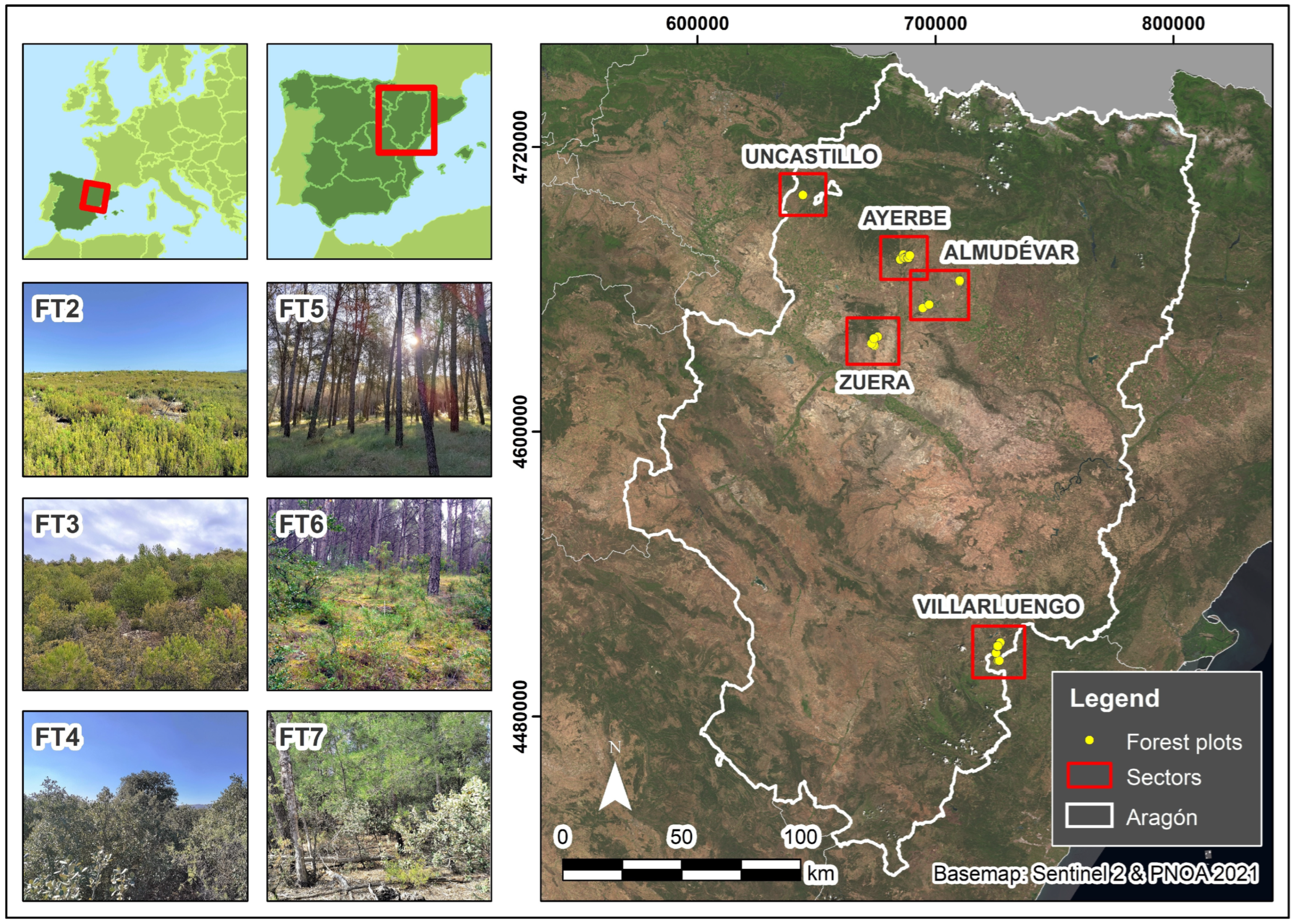
2.1. Study Area

The study was conducted across 43 forest plots of a 15 m circular radius, except for one plot of a 10 m circular radius (Table S1 of Supplementary Materials). These plots were selected from those previously utilized by Hoffrén et al. (2023) [26]. They were distributed across 5 sectors of the Autonomous Community of Aragón (NE Spain) as follows: Almudévar, Ayerbe, Uncastillo, Villarluengo, and Zuera (Figure 1). The prevailing climate in these sectors is Mediterranean with a continental influence, characterized by sporadic and irregularly distributed rainfall throughout the year, substantial daily and annual thermal gradients, and convective storms, which are frequent in late spring and summer. The sectors of Almudévar, Ayerbe, and Zuera are located in the Central Ebro Valley, where climatic conditions tend to be more extreme, resembling steppe-like conditions with cold winters, very hot and dry summers, low precipitation, and a high probability of drought periods. On the other hand, the Uncastillo sector, situated to the north of the Central Ebro Valley near the southern foothills of the Pre-Pyrenean range, experiences less extreme temperature gradients and higher rainfall. Finally, the Villarluengo sector, located in the Iberian range, features colder winters and milder summers compared to the other sectors due to its higher altitude [51]. All plots are characterized by typical Mediterranean vegetation well-adapted to the local climatic conditions, including shrublands and forest predominantly consisting of Aleppo pine (Pinus halepensis Mill.) and bog pine (Pinus nigra Mill.) mixed with an understory of oaks (Quercus coccifera L., Quercus faginea Lam., and Quercus ilex subsp. rotundifolia Lam.), boxwood (Buxus sempervirens L.), junipers (Juniperus oxycedrus L.), rosemary (Rosmarinus officinalis L.), and thymes (Thymus vulgaris L.). The climatic conditions, along with the characteristics of vegetation, and together with recent processes such as cropland abandonment and natural and systematic reforestation with pine species, lead to a high risk of forest fires. In fact, 3 out of the 5 sectors experienced large wildfires (>500 ha of burned area) in the last 30 years: Uncastillo and Villarluengo in 1994 and Zuera in 1995 and 2008. Although each forest plot had initially assigned a Prometheus fuel type as the ground truth (see Hoffrén et al., 2023 [26]), fuel types were reassigned during each visit, as plots could undergo changes in the dominant Prometheus type due to natural vegetation dynamics. The grassland fuel type (FT1) was not considered in this study due to its highly homogeneous and distinctive fuel structure. The center of each plot was determined using a Leica Viva® GS15 CS10 GNSS real-time kinematic global positioning system with centimeter-level accuracy.

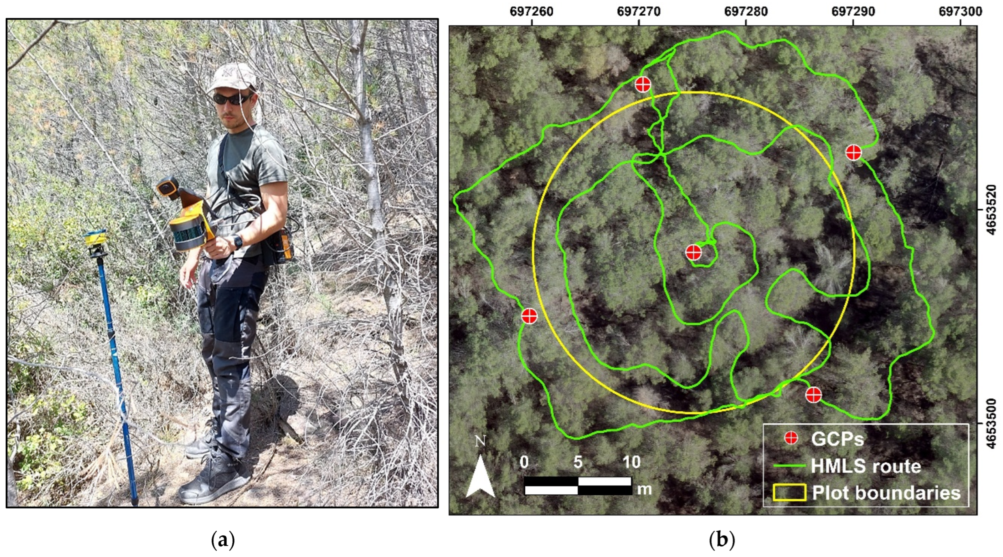
2.2. Data Acquisition and Preprocessing

HMLS data were collected at the end of May 2023 using a GeoSLAM ZEB-Horizon unit (GeoSLAM Ltd., Ruddington, UK) (Figure 2a), capable of scanning 300,000 points per second with a maximum scan range of 100 m and a 360° × 270° field of view. Scans were performed following methods similar to those described in Gollob et al. (2020) [45,52]. The scanning procedure commenced at the center of each plot, followed by an inner circular scan approximately 1 m from the plot’s center and an outer circular scan at the plot’s boundaries, pointing towards the center of the plot. Next, a detailed scan was performed within the plot in densely vegetated and shadowed areas to mitigate occlusion issues, concluding the scan at the starting point located at the plot’s center. An example of a typical scan path on a plot can be observed in Figure 2b. The scanning time for each plot was about 10–15 min (longer in denser plots). The interaction of the laser system with the vegetation generated highly dense three-dimensional point clouds, with an average point density of 63,148 points/m2 for all plots (detailed densities for each plot are presented in Table S1 of the Supplementary Materials). Since the HMLS system did not incorporate an inertial measurement unit, data were collected in local coordinates (i.e., the center of the plot had coordinates XY 0,0) and were subsequently georeferenced to a coordinate reference system. To achieve this, 5 ground control points (GCPs) were established in each plot before the start of the scans with the Leica Viva® GS15 CS10 GNSS. One GCP was positioned at the center of the plot, and the remaining four were placed at each of the cardinal points of the plot’s boundaries (Figure 2b). During the scans, the HMLS remained static and at ground level on each GCP for at least 10 seconds to record the local coordinates, which were then matched with the coordinates obtained from the GNSS at the same GCP. For data preprocessing, the proprietary software GeoSLAM Connect v.2.3.0 was employed. It involved the conversion of scans into LAS files and georeferencing local coordinates to a coordinate reference system (EPSG: 25830–ETRS89/UTM zone 30N). For the latter, the ‘Stop and Go alignment’ tool was utilized, facilitating the association of the local coordinates registered with the HMLS to the coordinates recorded with the GNSS at each GCP in the coordinate reference system. The mean georeferencing error for all plots was 0.161 m (detailed results are provided in Table S1 of the Supplementary Materials).

2.3. Ground Points Classification

The georeferenced point clouds were classified into ground and non-ground points for the generation of digital elevation models (DEMs) and height normalization. This process is a key step for ensuring that subsequent analyses are accurate, given the very high point cloud density of the HMLS data. To accomplish this, three different ground classification algorithms commonly used in forestry were tested as follows: the ‘lasground’ algorithm of LasTools (Rapidlasso GmbH, Gilching, Germany), the multiscale curvature classification (MCC) algorithm [53], and the cloth simulation filter (CSF) algorithm [54]. The software used for this purpose was ArcMap v.10.7.1 (ESRI, 2019) for LasTools, MCC-LiDAR v.2.1 [52] for the MCC, and the lidR package [55,56] of the R environment [57] for the CSF. The classification could be applied without reducing the original point cloud densities in the cases of LasTools and the CSF, but with the MCC, the point clouds had to be decimated to 1000 points/m2 due to computational limitations. The points classified as ground by the three algorithms were used to generate DEMs with a spatial resolution of 0.20 m by the TIN-to-raster interpolation method [58] using the ‘rasterize terrain’ function of the lidR package. Subsequently, the elevation values were extracted from the DEMs through the random sampling of 2000 points, and they were compared with each other to compute the mean height error for each algorithm. The DEMs from the algorithm with the lowest mean error were selected to normalize the heights of the point clouds. This was achieved using the ‘normalize heights’ function of the lidR package. Finally, normalized points with negative height values or exceeding 40 m (i.e., outliers) were removed using the ‘filter poi’ function of lidR.

2.4. Voxelization and Fuel Load Quantification

Estimation of the fuel load was performed by calculating the volume of the normalized point clouds. For this purpose, a voxelization process was conducted, which has been reported as a well-suited approach for estimating forest fuels (e.g., [59,60,61,62]) and allows for simplifying the huge amount of data coming from ground-based LiDAR systems [63,64,65,66,67]. In doing so, the effect of uneven point distributions, many of which tend to be located closer to the sensor, is normalized [64,65]. The first step prior to the voxelization process was to consider the resolution of the voxels so that they could accurately describe the heterogeneous structure and distribution of fuel loads without a loss of information. Considering the average point cloud densities, voxels were generated at a 5 cm grid resolution using the VoxR package for R [65,68]. Before that, the points considered as noise were filtered out using the Statistical Outliers Removal (SOR) filter available in the VoxR package. The SOR filter considers a point to be noise if it is at a distance to its nearest neighbors greater than the mean distance of the entire point cloud plus 1.5 times the standard deviation of the other points [68]. As a result of voxelization, each plot was composed of a collection of filled and empty voxels in the XYZ space (Figure 3). Filled voxels indicated the presence of at least one point of the point cloud, while empty voxels denoted an absence of points.
The total volume for each plot in each 5 cm height stratum was computed as the sum of the filled voxels in each stratum multiplied by their volume (Equation (1)), following the methods adopted by Martínez-Rodrigo et al. (2022) [66]. In order to take into account, with a cautious approach, the measurement accuracy of the instrument, which is around 1–3 cm, for subsequent analyses, the first voxelized stratum (i.e., voxels between 0 and 5 cm of height) was not considered to ensure an exclusion of returns that may belong to the ground and not to the fuel. The volume of each height stratum was calculated in absolute (m3/m2) and relative (% of the total) terms. Additionally, the total volume of the fuel load was calculated for each height threshold of the Prometheus model: below 0.60 m for the low shrub (LSh) stratum, between 0.60–2 m for the medium shrub (MSh) stratum, between 2–4 m for the high shrub (HSh) stratum, and above 4 m for the tree stratum (Tr), for quantifying the average fuel load for each fuel type.
V O L s = V O X s   × ( 0.05 ) 3
where VOL represents the total volume in absolute (m3/m2) and relative (% of the total) terms in the s height stratum, and VOX represents the filled voxels in the s height stratum.

3. Results

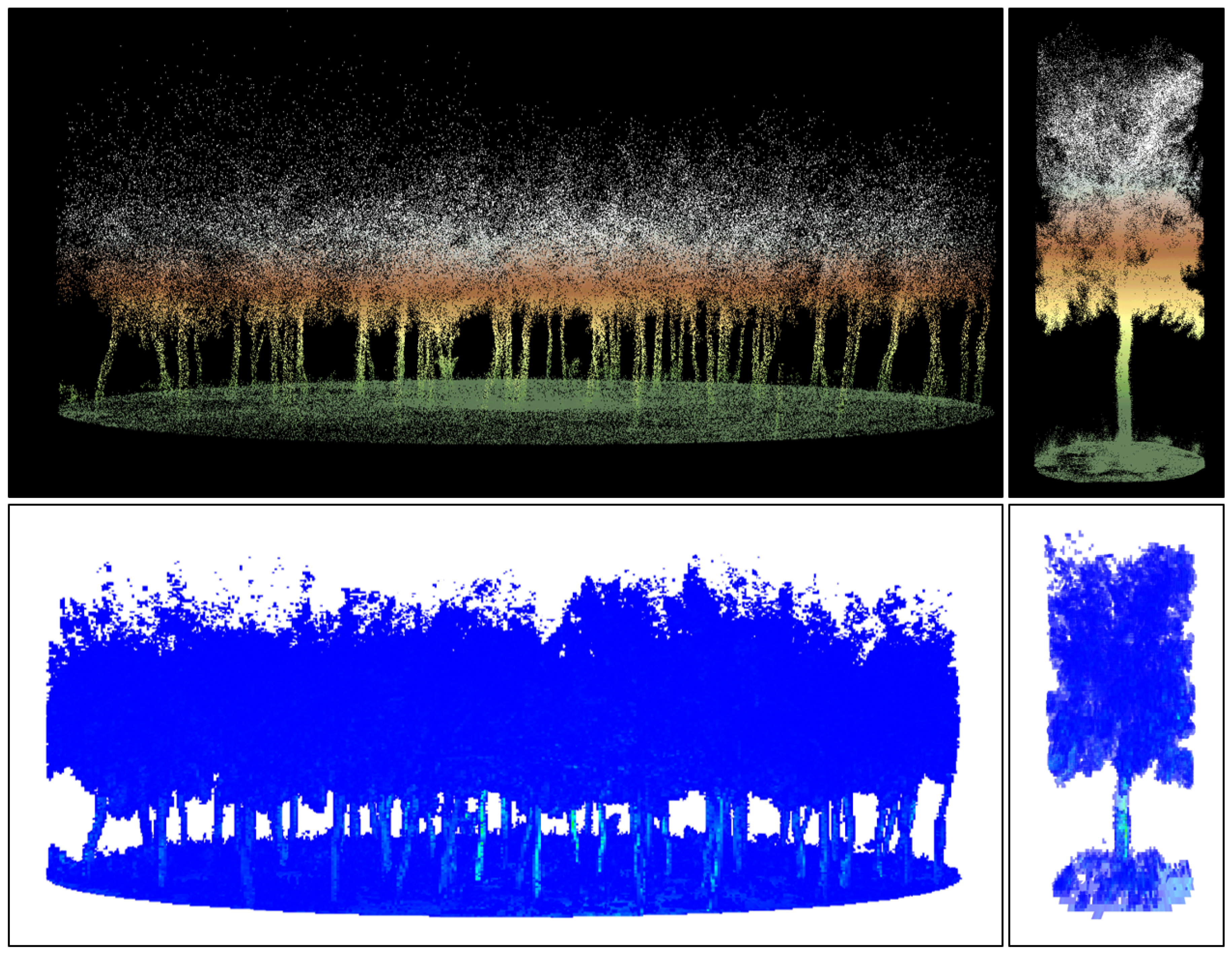
3.1. Visual Analyses of the Processed Point Clouds

A preliminary assessment of the differentiation capability between the Prometheus fuel types was conducted through a visual analysis of the point clouds. Figure 4 illustrates the structural heterogeneity of vegetation at both the plot and transect scales by fuel type. It can be observed that the acquired and processed data successfully represent the vertical distribution of vegetation, even in the upper strata (e.g., canopies), which are further away from the ground, where data are acquired. The LSh, MSh, and HSh strata (i.e., shrub strata) are predominant in FT2, FT3, and FT4, respectively. In addition, some scattered larger shrubs or small trees can be found in the FT2 and FT3 plots, while FT4 exhibits a greater spatial continuity of tall shrubs. In FT5, the point cloud clearly represents the tree profile and the absence of an understory. Continuity of vegetation can be observed between the lower and upper strata for the tree fuel types, as in FT6, but to a lesser extent compared to FT7, where the fuel reaches the maximum structural volume and the highest stand compactness.

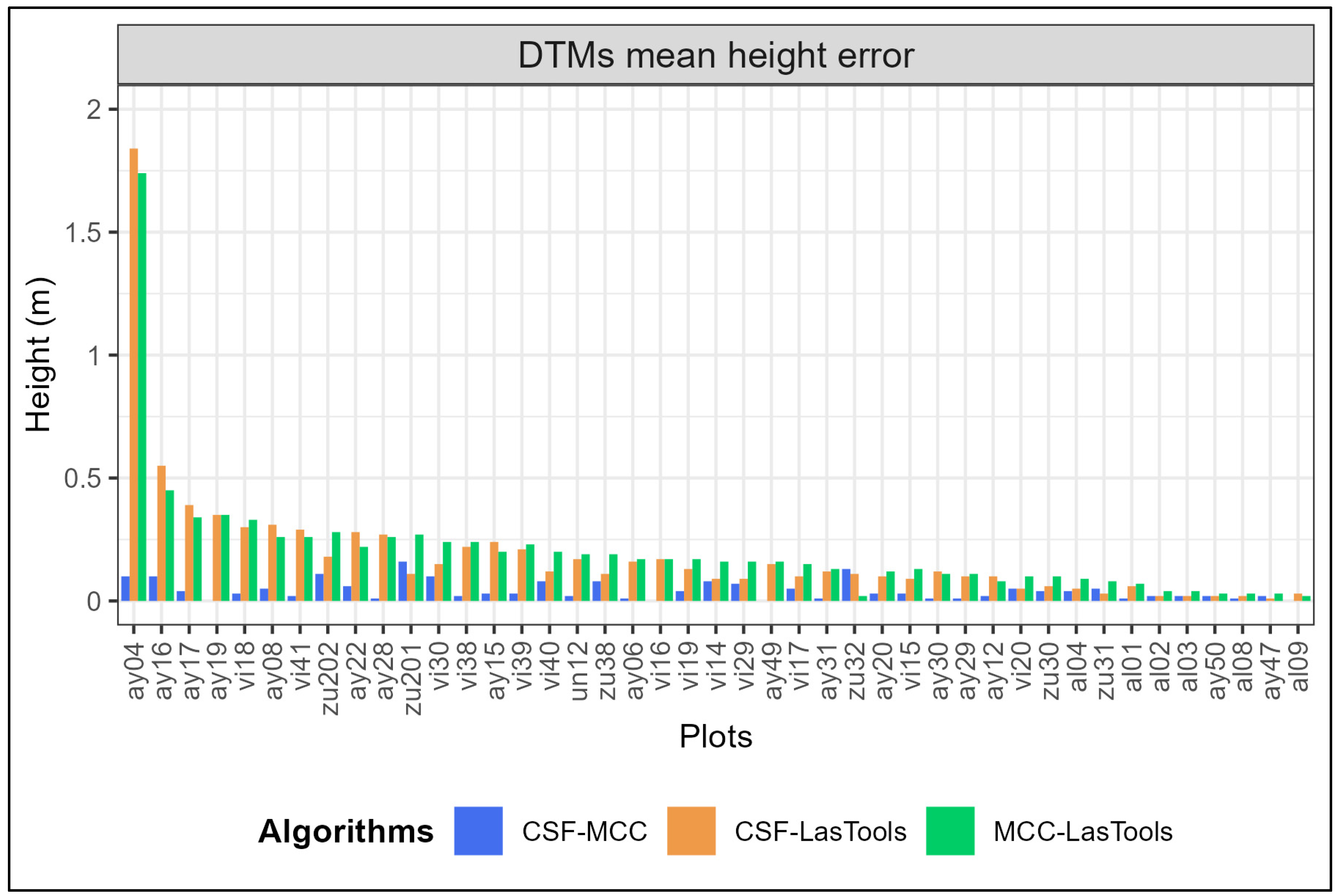
3.2. Selection of the Ground Points Classification Algorithm

Figure 5 depicts the results of the comparative analyses of the mean height error for each plot and between algorithms. The detailed results can be found in Table S2 of the Supplementary Materials. There were minimal differences in the height values extracted from the MCC and CSF (mean error = 4 cm, standard deviation = 4 cm), whereas, with LasTools, the differences with the other two algorithms were slightly larger (LasTools–MCC: mean error = 19 cm, standard deviation = 28 cm; LasTools–CSF: mean error = 20 cm, standard deviation = 26 cm). Regarding the classification process, the MCC took considerable time to process the decimated point cloud, while LasTools and the CSF processed the complete point cloud in less time. Therefore, based on these results, the CSF algorithm was chosen as the most suitable for filtering and classifying the point clouds into ground and non-ground points to normalize the heights of the point clouds.

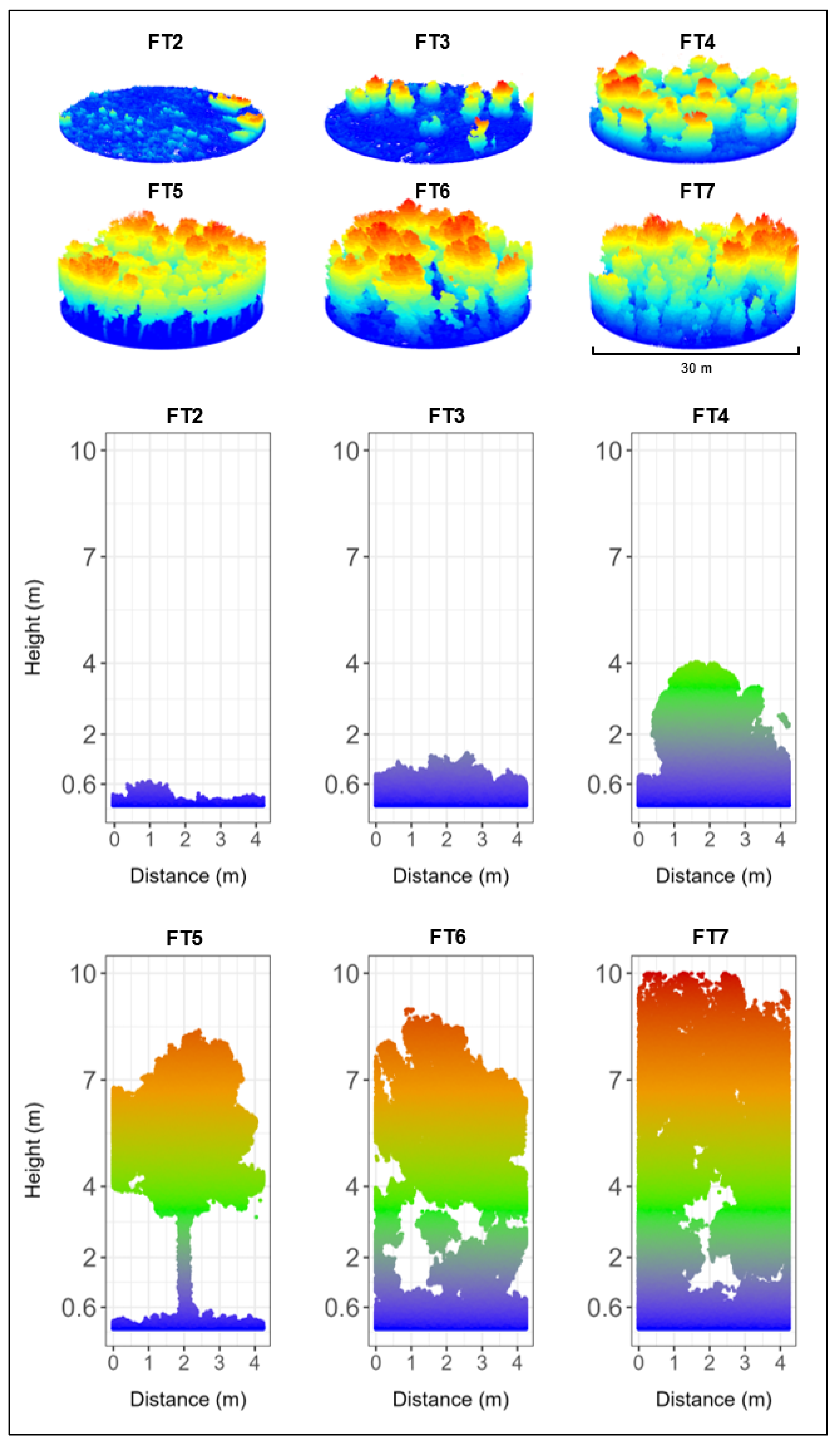
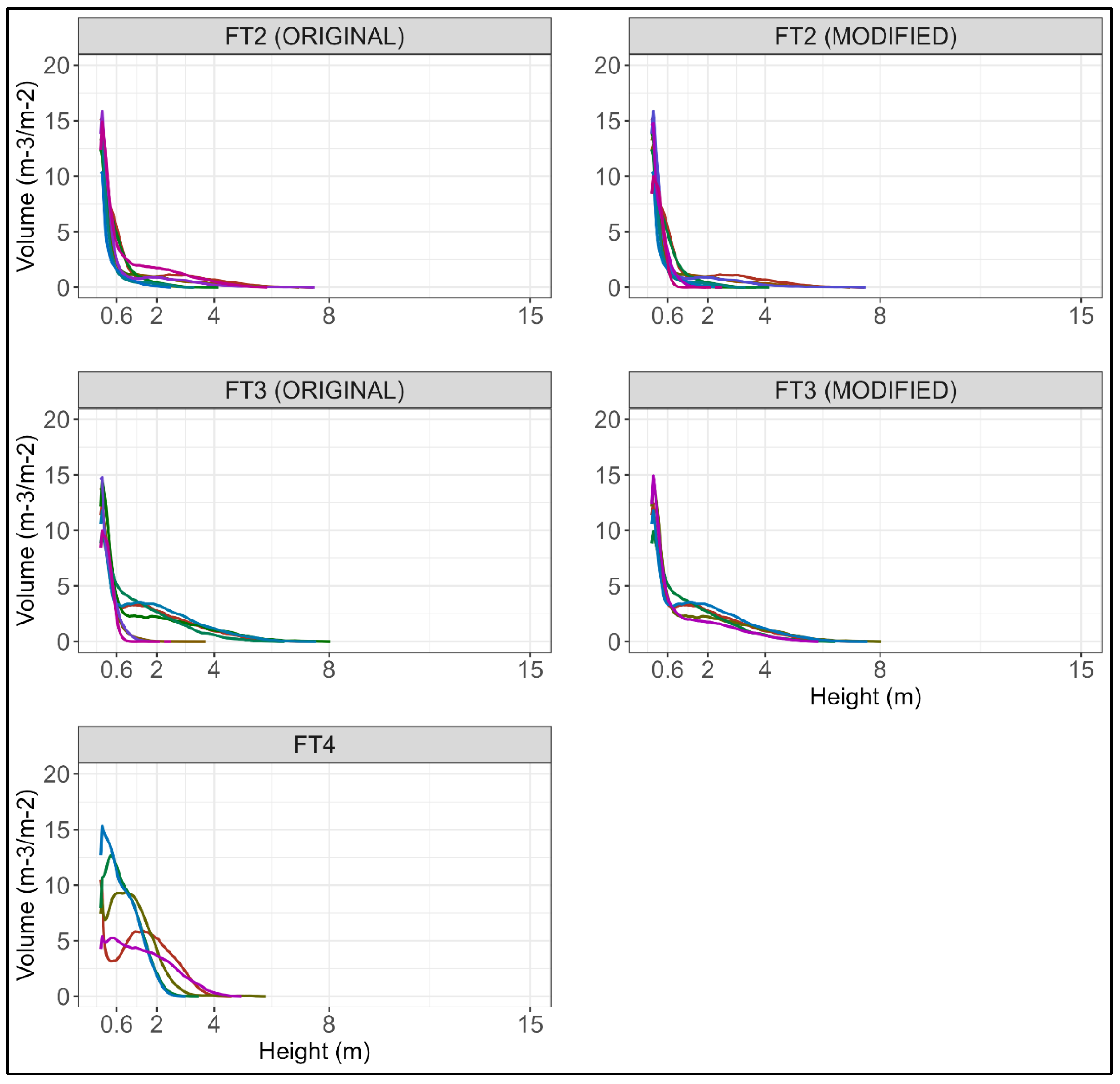
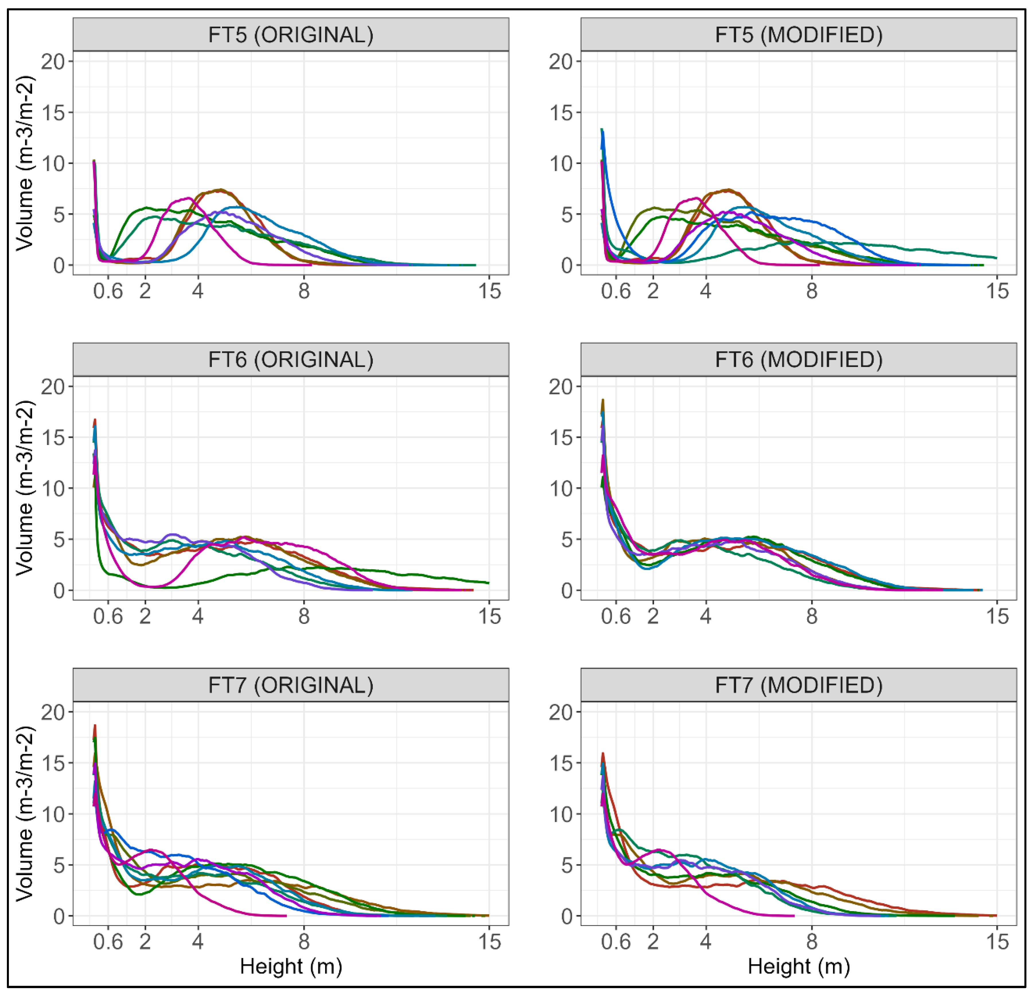
3.3. Definition of Prometheus Fuel Types

The vertical distribution of the fuel volume every 5 cm enabled the definition of specific distributions of the Prometheus fuel types for each forest plot (see Figures S1–S3 of the Supplementary Materials), facilitating the detection of plots with inaccurately estimated fuel types in the field.
In general terms, the Prometheus shrub fuel types (FT2, FT3, and FT4) exhibit a unimodal distribution, except for some cases in FT4, with peaks in the LSh stratum and a gradual decrease in fuel towards the higher strata, nearly diminishing in the MSh stratum (Figure 6). In FT2, the fuel is primarily concentrated in the LSh stratum, with only a few plots showing a slight increase between 0.60 and 4 m, likely due to scattered low trees within those plots, though it does not significantly alter the overall distribution. In FT3, the decline in fuel load is less abrupt than in FT2 within the LSh stratum but stabilizes in the MSh stratum before gradually decreasing to the Tr stratum. The distribution of FT4 differs slightly from that of FT2 and FT3, with the peak found in both the LSh and MSh strata. Moreover, there is a higher volume of fuel in the MSh stratum. Some plots exhibit a bimodal distribution, with peaks in both the LSh and MSh strata. These distributions in FT4 suggest a continuity of the vertical fuel structure below 4 m, characteristic of this fuel type. Based on these findings, a total of four shrub-type plots with inaccurately estimated fuel types in the field were identified. One plot, initially classified as FT2 (‘vi40’), did not align with the average distribution for this fuel type, as it exhibited a higher fuel volume in the MSh stratum, aligning more closely with FT3. Consequently, the ground truth was changed to this fuel type. Additionally, three plots classified as FT3 (‘vi17’, ‘zu30’, and ‘zu31’) were reclassified as FT2, as their volume distribution showed an abrupt decrease in fuel from the MSh stratum, better fitting with the FT2 distributions. In the case of the FT4 plots, no modifications were made.
Regarding the Prometheus tree fuel types, FT5 displays a distinctly bimodal distribution, with a primary peak in the LSh stratum and a secondary peak starting in the HSh stratum and continuing into the Tr stratum or originating directly in the Tr stratum, with a minimal fuel load volume in the MSh stratum. The distribution of FT6 exhibits a peak in the LSh stratum, followed by a decrease in the MSh stratum and a slight increase in the HSh stratum, culminating in a gradual decline from the Tr stratum. FT7 exhibits a very similar distribution to FT6, except for a more consistent volume along the MSh and HSh strata before declining from the Tr stratum. This indicates greater volume in the intermediate strata and consequently, more vertical continuity of the fuel load, characteristic of this type. These findings revealed misidentifications of ground truth in six tree-type fuel plots. Two plots, initially categorized as FT6 (‘ay12’ and ‘ay49’), were reassigned to FT5 due to the distinct bimodality of their distributions and minimal volume present in the MSh and HSh strata. Another plot initially labeled as FT6 in the field (‘ay31’) was corrected to FT7, as it demonstrated a consistent fuel volume between the LSh and MSh strata. Moreover, three plots originally labeled as FT7 (‘ay06’, ‘ay19’, and ‘ay28’) were modified to FT6, as their distributions indicated a decrease in volume in the MSh stratum, suggesting less vertical continuity of vegetation. Finally, a plot labeled as FT7 (‘vi41’, corresponding to the pink line in the FT7 plots of Figure 7) displayed a distinctive signature compared to others of the same fuel type. While this plot could potentially fall between FT4 and FT7 due to its clear bimodality resembling some FT4 plots, the significant fuel load from the Tr stratum, persisting until approximately 8 meters, suggests excessive height for the FT4 plot. Consequently, the ground truth was not modified, assuming it to be a FT7 plot with a low tree height.

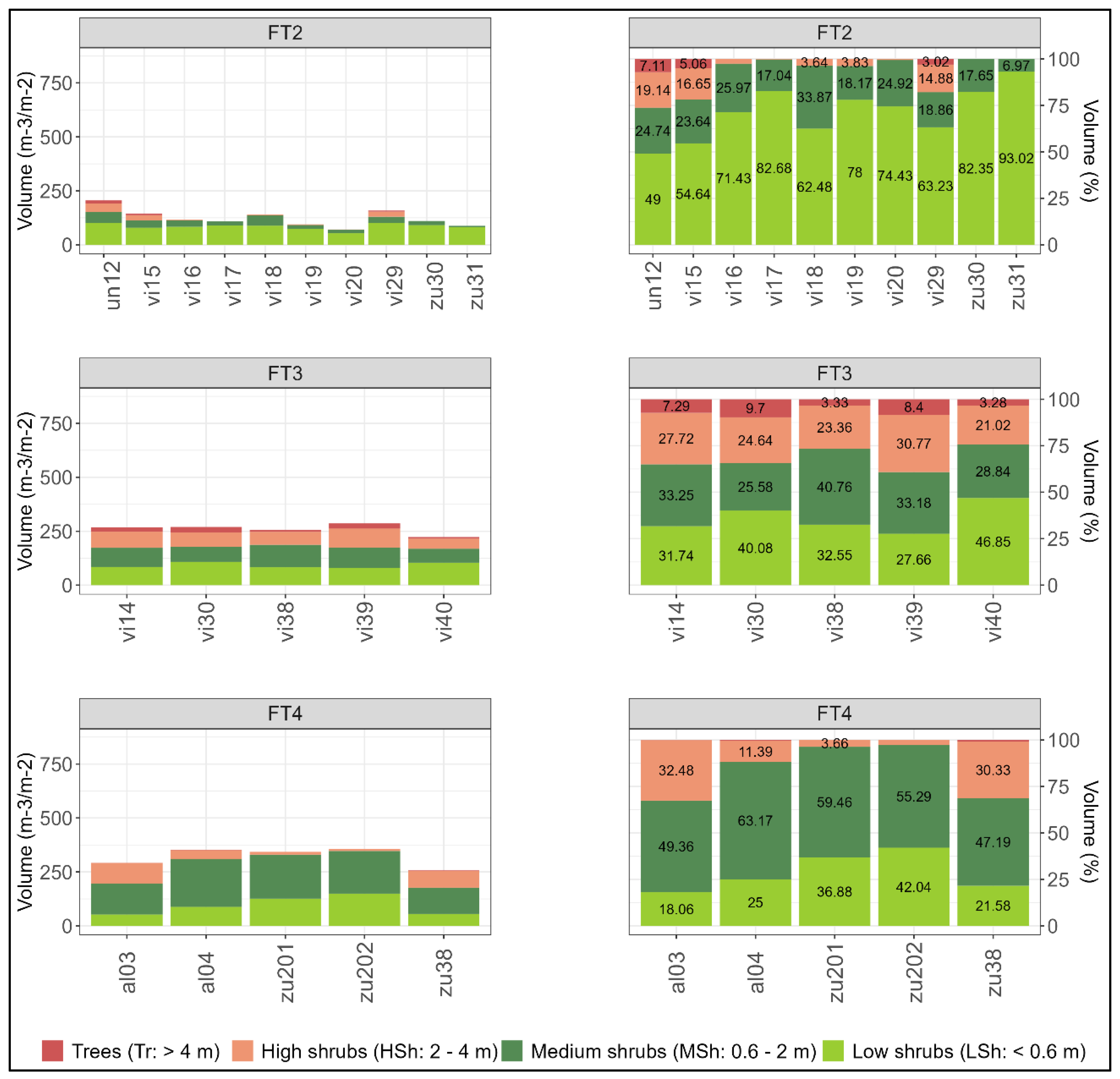
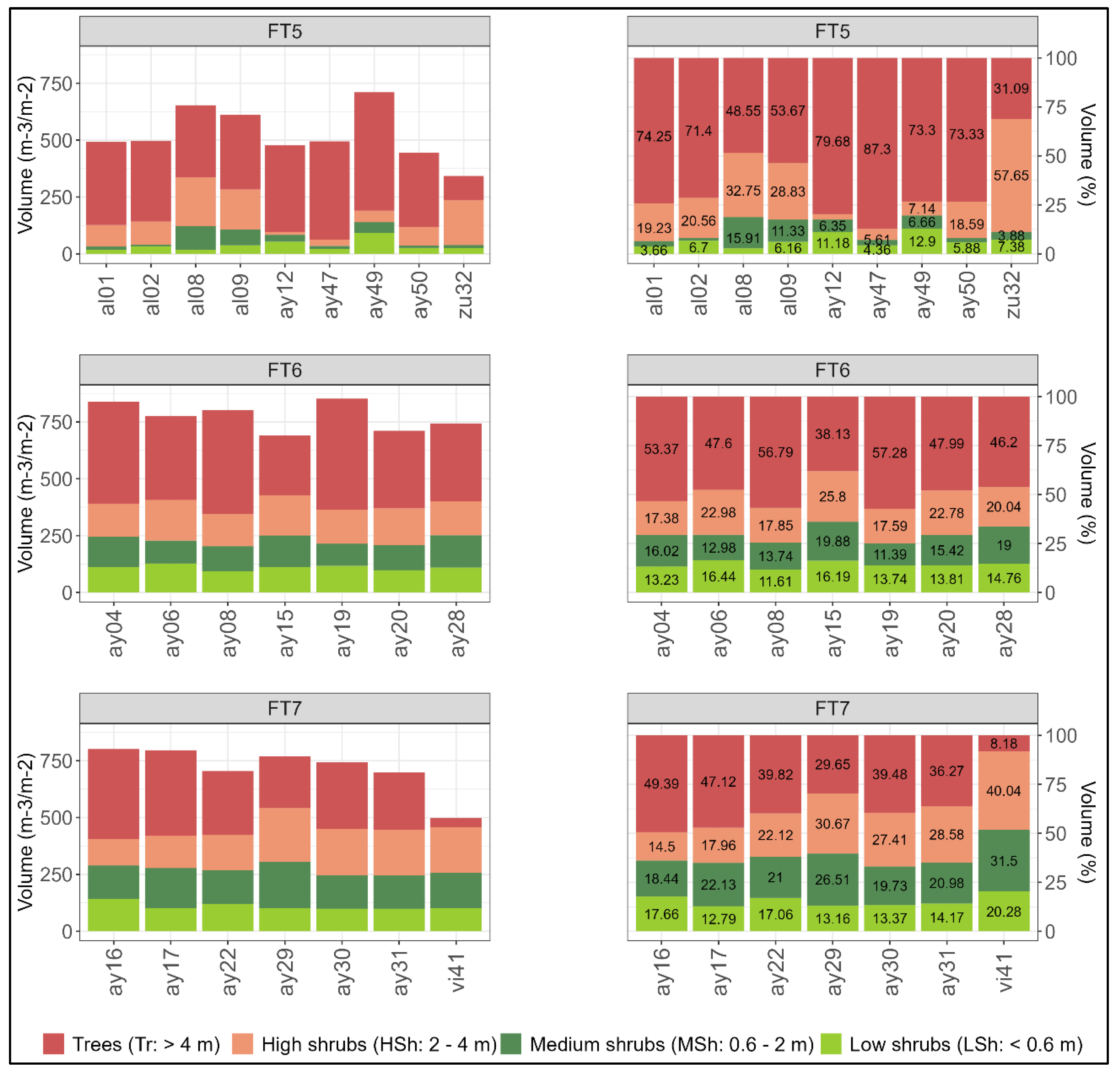
3.4. Quantification of Prometheus Fuel Load

The quantification of fuel load by Prometheus height strata confirmed the corrections made to the ground truth in the 10 forest plots. The results presented below are grouped by the fuel types modified from the HMLS data, as mentioned in the previous section. Figure 8 illustrates the fuel volume of each Prometheus shrub fuel type, revealing a generally progressive increase in the total volume from FT2 to FT4; specifically, the volume is less than 250 m3/m2 in FT2, slightly over 250 m3/m2 in FT3 (except for one plot: ‘vi40’), and somewhat higher than 250 m3/m2 in FT4. Plot ‘vi40’ was misclassified as FT2 in the field and is the only one among FT3 that does not exceed 250 m3/m2 of the total volume. This suggests that this plot could be on the border between FT2 and FT3. However, the percentage of volume contained in the MSh and HSh strata in this plot is quite high (>20%), resembling the percentages of FT3 plots more closely. Regarding the percentage of volume in each Prometheus stratum, a clear dominance of the LSh stratum is observed in FT2 (>50% of the total volume in all plots except for one), with greater parity in FT3 but with more significant proportions in the two lower strata, and a predominance of the MSh stratum in FT4. As expected, the percentage of the total volume in the Tr stratum is almost negligible in the three shrub types. Only three FT2 plots have volume in the HSh and Tr strata, which are related to the small volume increments seen in these strata in Figure 5 and explained before. There is a higher volume percentage in the Tr stratum in the FT3 plots, but they are still low values, while there is hardly any in FT4. Finally, it is worth noting that the volume of the plots where the ground truth was corrected (‘vi17’, ‘vi40’, ‘zu30’, and ‘zu31’) fits quite well within their respective new groups.
In the Prometheus tree fuel types, there is a lower volume of fuel load in FT5 (<750 m3/m2) due to the absence of understory and a slightly higher volume in the FT6 plots compared to FT7 (Figure 9) due to a greater volume of tree canopies in the former. In general terms, the dominant stratum in these types is the Tr stratum, reaching the highest percentages in the FT5 plots. The FT7 plots have greater uniformity in the volume contained in each Prometheus stratum, although some plots show similar volume percentages in the MSh and HSh strata to others identified as FT6 (e.g., ‘ay16’ and ‘ay17’). This may be an indicator of the high complexity of the vertical fuel structure in both types. However, in the FT6 plots, there are no cases of a volume percentage higher than 20% in the same plot in both the MSh and HSh strata, while this is a characteristic in most FT7 plots, suggesting a greater vertical continuity of fuel between the strata in the latter. Regarding FT5, the amount of volume in the LSh and MSh strata is very low, and appreciable amounts are only found in plots ‘al08’, ‘al09’, ‘ay12’, and ‘ay49’. In the case of the former two, it is due to a higher percentage of MSh strata, although this percentage is not high. The latter two were labeled in the field as FT6 because they had a higher volume of fuel in the MSh stratum compared to the other FT5 plots. However, their volume by Prometheus height strata seems to fit better in FT5, confirming the corrections made previously. Plot ‘zu32’ has the most distinctive volume distribution of all FT5 plots, as the dominant stratum is the HSh stratum, assuming that this is a FT5 plot with a low tree height. On the other hand, the volume of plot ‘ay31’, whose fuel type was labeled as FT6 in the field, fits quite well as FT7. Plots ‘ay06’, ‘ay19’, and ‘ay28’, which transitioned from FT7 to FT6, also seem to fit better with their new type. Lastly, it is confirmed that plot ‘vi41’ is a ‘low FT7’ plot since it has very little volume in the Tr stratum but a lot in the HSh stratum. Its distribution closely resembles those of FT4 plots, although with significantly more volume in the upper strata, so it might not be appropriate to be labeled as FT4.

4. Discussion

In the current context of increasing exposure to wildfires, it is necessary to develop plans to mitigate their negative effects on the environment. An effective step is to correctly identify fuel types in the field to accurately model fire behavior in larger areas. However, forest stands are often structurally complex and present mixed features of several fuel types, especially in the Mediterranean region, making the in situ estimation of fuels challenging at times. This study has relied on a HMLS system to address this challenge, as its ability to obtain detailed data on forest vertical and horizontal structure allows for a more precise characterization of vegetation and the definition of Prometheus fuel types at the plot level. Thanks to the large amount of data involved, the corrections made to incorrectly identified fuel types in the field were successful, resulting in 10 out of the 43 plots changing their assigned fuel type, which could explain some of the confusion between similar fuel types observed in Hoffrén et al. (2023) [26]. Additionally, the proposed methodology, based on the use of a HMLS system, provides an efficient alternative for the estimation and correction of fuel types in the field in Mediterranean forest environments. Overall, the results show that voxelization of the very-high-density three-dimensional point clouds from the HMLS data allowed the identification of specific distributions of the vertical fuel volume for each Prometheus fuel type, while quantification of the fuel volume by Prometheus height strata validated the information provided by the distributions.
The CSF algorithm was the most suitable for the classification of the ground points. Filtering is a key process to normalize the heights and ensure the greatest accuracies in the subsequent voxelization and fuel volume estimation. This algorithm has already been used in previous studies that have employed HMLS systems (e.g., [37,45]), as well as TLS systems (e.g., [63,69]) and other MLS systems (e.g., [44]). The results of the centimetric-scale voxelization (5 cm) appear to be adequate for better identifying the vertical distribution of fuels and accurately estimating the Prometheus fuel types without loss of information on the structural complexity of the forest stands. Although the voxel size will depend on the research objectives and the quality of the data [65], several studies using ground-based LiDAR systems have employed small-sized voxels for volume estimation with satisfactory results. For instance, when using the TLS system, Lecigne et al. (2018) [65] noticed that smaller voxels were more suitable for capturing fine changes in tree features compared to larger voxel sizes, which is crucial when working in structurally complex environments such as Mediterranean forests. Yan et al. (2019) [70] generated voxels of a 20 cm size for the crown volume estimation from MLS-derived point clouds. Voxel sizes of 10 cm have also been used to estimate forest fuel characteristics with a TLS system [62] and stand structural features with the HMLS system [66]. In this study, the volume of fuel load has been calculated directly from the voxels, but it can also be estimated indirectly. For instance, a voxel-derived index called the PDI (the plant diversity index) was proposed by Puletti et al. (2021) [71], which relates the number of filled voxels to the total number of voxels within the same height stratum, resulting in the satisfactory estimation of the vertical distribution of fuel volume. Despite the small voxel size used for the voxelization and the very high density of the point clouds, the process was relatively fast and allowed for more efficient management of the vast amount of data collected with the HMLS. In this regard, voxels allow for the removal of some unwanted effects typical of ground-based LiDAR systems, such as occlusion or differences in point cloud densities, which can introduce bias in the characterization of fuel structure. This process of discretizing point clouds also helps in monitoring forest changes over different time periods [72,73,74], which could be valuable for detecting progressive changes in the fuel types over time due to natural vegetation growth. In this sense, working directly with the point cloud would have been computationally more demanding, as the extraction of structural metrics to estimate the distribution and density of forest structure is typically done at the pixel or plot level. Thus, this study proposes a simpler methodology for better defining fuel types and correcting those that were incorrectly estimated in the field.
Among the various platforms of ground-based LiDAR systems, this study has utilized a HMLS in a novel application in forestry. Overall, the results of the modifications for incorrectly estimated fuel types in the field are satisfactory and underscore the value of HMLS systems for quantifying the fuel load volume and precisely defining Prometheus fuel types. However, certain limitations related to intrinsic system errors and to the estimation of fuel volume in quantitative units (m3/m2) must be considered. On one hand, the system itself may exhibit jitter errors that are challenging to control, necessitating the acceptance of some uncertainty in the recorded data. Additionally, the manner in which scans are conducted by the user can influence data accuracy. Therefore, methods from previous studies, such as predefined routes, sensor orientation, and designated starting and ending scanning points, were followed in order to minimize uncertainty (e.g., [40,45,48,52]). Furthermore, the voxelization process helped to homogenize the point clouds, thus mitigating bias [65]. On the other hand, estimating the fuel volume in quantitative units may not always be entirely satisfactory. For example, some FT6 and FT7 plots exhibited very similar vertical fuel distributions (Figure 9), potentially leading to confusion between the different types, even when working at centimetric scales, as in this study. Moreover, the voxels were computed for the entire point cloud without differentiation of the objects from which they were returned. They lacked information related to the presence of different vegetation parts, such as foliage, branches, trunks, or bark, which are relevant for wildfire considerations. In this context, some studies have attempted to categorize voxels according to their class to enhance fuel quantification (e.g., [59,60]). However, this can be a complex task in forest environments of very high structural heterogeneity, where different fuel classes are intermingled. Another limitation is the inability to differentiate between live and dead fuel from the raw point cloud data. Some HMLS systems allow the collection of data in combination with RGB images, which could aid in distinguishing between both types of fuel, although the processing could be time- and resource-intensive. Nevertheless, it would enable an improved fuel characterization and more accurate fire spread modeling. Despite these limitations, the HMLS system has facilitated the identification of plots with incorrectly estimated fuel types in the field and corrected them to their closest type. Confusions observed in the vertical distributions of fuel load volume (Figure 6, Figure 7, Figure 8 and Figure 9) align with previous studies, which also reported inaccuracies in those fuel types using other remote sensing methodological approaches (e.g., [21,22,24,25]). The categories that underwent changes here also presented confounding issues in Hoffrén et al. (2023) [26], where the worst classified types were FT3 and FT6. In this study, Figure 6 and Figure 7 confirm the existence of discrepancies in these two fuel types, with three plots initially assigned as FT3 in the field through visual analysis being modified to FT2, while three other FT6 plots had their assignment adjusted from FT6 to FT5 (two plots) and to FT7 (one plot).
The main confusion between fuel types may be due to the incorrect estimation of the volume of shrub or understory, i.e., understory fuels. In shrub fuel types, it determines the maximum height, while in tree fuel types, it defines the degree of vertical continuity between the understory and the canopies. Although ground-based LiDAR systems have demonstrated greater capabilities in identifying understory fuel than other systems [75,76], leveraging alternative remote sensing platforms could enhance the estimation of understory fuels. For instance, Hillman et al. (2021) [63] observed that LiDAR sensors mounted on unmanned aerial vehicles (LiDAR UAVs) effectively estimated understory fuels in a dry sclerophyll forest, achieving accuracy comparable to the TLS systems. Conversely, Hyyppä et al. (2020) [43] demonstrated that above-canopy LiDAR UAVs struggle to identify forest understory attributes, while under-canopy LiDAR UAVs can achieve a similar performance to ground-based LiDAR systems [43,77]. Therefore, LiDAR UAVs offer a viable alternative for fuel-type identification, as they can cover larger areas and provide valuable data. However, they may be subject to more restrictive regulations and operational challenges in dense and complex forests. HMLS data also offer the potential to obtain data over extensive areas, albeit requiring more time and effort. In addition, some forest plots may be inaccessible due to their extremely high vegetation density, particularly in Mediterranean forests. Despite these challenges, HMLS systems offer advantages such as a larger scanning area than the TLS system [40], flexibility in mobility within the forest, and the ability to georeference data indirectly with GCPs or directly with an inertial measurement unit. Consequently, based on our findings, HMLS systems should be regarded as promising tools to enhance field fuel load estimations. This improvement will contribute to better forest fuel modeling, thereby aiding in the development of effective forest fire prevention and mitigation plans.

5. Conclusions

Knowing the spatial distribution of forest fuels is a crucial step to understanding fire behavior in a hypothetical wildfire. In this sense, ground-based LiDAR systems can provide very detailed information on the vertical distribution of forest fuels in exceptional detail, which can be of great interest in improving the field estimation of fuel types. The results of this study conclude that HMLS systems are capable of detecting fuel loads in centimeter-scale height strata in heterogeneous forest plots. With this information, it is possible to determine the fuel type to which the plot belongs, even when there is a mixture of characteristics of different fuel types, a situation quite common in Mediterranean forest environments. This study has focused on the Prometheus model, but the approach could be applied to other relevant fire models. Thus, a better identification of fuel types can enhance the ground truth of classification models, enabling more accurate modeling of fire behavior in larger areas. Ultimately, this contributes to improved wildfire prevention and mitigation in the territory.

Supplementary Materials

The following supporting information can be downloaded at: https://www.mdpi.com/article/10.3390/fire7020059/s1, Figure S1: Vertical distribution of the fuel volume of each forest plot every 5 cm (1/3); Figure S2: Vertical distribution of the fuel volume of each forest plot every 5 cm (2/3); Figure S3: Vertical distribution of the fuel volume of each forest plot every 5 cm (3/3); Table S1: Name, location, point cloud density, and mean georeferenced error of the forest plots. Plot ‘zu38’ has a 10 m circular radius; Table S2: Mean height error (in meters) between the three ground classification algorithms tested in the study for each plot.

Author Contributions

Conceptualization, R.H., M.T.L. and J.d.l.R.; methodology, R.H., M.T.L. and J.d.l.R.; software, R.H.; validation, R.H., M.T.L. and J.d.l.R.; formal analysis, R.H.; investigation, R.H., M.T.L. and J.d.l.R.; data curation, R.H.; writing—original draft preparation, R.H.; writing—review and editing, R.H., M.T.L. and J.d.l.R. All authors have read and agreed to the published version of the manuscript.

Funding

This work was supported by the Spanish Ministry of Science, Innovation, and Universities through an FPU predoctoral contract granted to R.H. [FPU18/05027]; by the Government of Aragón (Geoforest S51_23R co-financed with FEDER ‘Construyendo Europa desde Aragón’); and by the University Institute for Research in Environmental Sciences of Aragón (IUCA) of the University of Zaragoza, for covering the cost of renting the GeoSLAM ZEB-Horizon HMLS unit and the GeoSLAM Connect v.2.3.0 software.

Institutional Review Board Statement

Not applicable.

Informed Consent Statement

Not applicable.

Data Availability Statement

Datasets are available on request.

Acknowledgments

The authors would like to thank Grafinta S.A. (Av. Filipinas 46, 28003 Madrid, Spain) for providing the GeoSLAM ZEB-Horizon HMLS unit and the GeoSLAM Connect v.2.3.0 software, as well as for their continuous support and guidance, especially David Cruz. The authors also thank Darío Domingo for his support in the fieldwork.

Conflicts of Interest

The authors declare no conflicts of interest.

References

  1. Bowman, D.M.J.S.; Balch, J.K.; Artaxo, P.; Bond, W.J.; Carlson, J.M.; Cochrane, M.A.; D’Antonio, C.M.; Defries, R.S.; Doyle, J.C.; Harrison, S.P.; et al. Fire in the Earth System. Science 2019, 324, 5926. [Google Scholar] [CrossRef] [PubMed]
  2. Pausas, J.G.; Keeley, J.E. A burning story: The role of fire in the history of life. Bioscience 2009, 59, 593–601. [Google Scholar] [CrossRef]
  3. Nocentini, S.; Coll, L. Mediterranean forests: Human use and complex adaptive systems. In Managing Forests as Complex Adaptive Systems. Building Resilience to the Challenge of Global Change; Messier, C., Puettmann, K.J., Coates, K.D., Eds.; Routledge: London, UK, 2013; pp. 214–243. [Google Scholar]
  4. Jones, M.W.; Abatzoglou, J.T.; Veraverbeke, S.; Andela, N.; Lasslop, G.; Forkel, M.; Smith, A.J.P.; Burton, C.; Betts, R.A.; van der Werf, G.R.; et al. Global and regional trends and drivers of fire under climate change. Rev. Geophys. 2022, 60, e2020RG000726. [Google Scholar] [CrossRef]
  5. Rovithakis, A.; Grillakis, M.G.; Seiradakis, K.D.; Giannakopoulos, C.; Karali, A.; Field, R.; Lazaridis, M.; Voulgarakis, A. Future climate change impact on wildfire danger over the Mediterranean: The case of Greece. Environ. Res. Lett. 2022, 17, 045022. [Google Scholar] [CrossRef]
  6. Ruffault, J.; Curt, T.; Moron, V.; Trigo, R.M.; Mouillot, F.; Koutsias, N.; Pimont, F.; Martin-StPaul, N.; Barbero, R.; Dupuy, J.L.; et al. Increased likelihood of heat-induced large wildfires in the Mediterranean Basin. Sci. Rep. 2020, 10, 13790. [Google Scholar] [CrossRef] [PubMed]
  7. Varela, V.; Vlachogiannis, D.; Sfetsos, A.; Karozis, S.; Politi, N.; Giroud, F. Projection of forest fire danger due to climate change in the French Mediterranean region. Sustainability 2019, 11, 4284. [Google Scholar] [CrossRef]
  8. Ascoli, D.; Moris, J.V.; Marchetti, M.; Sallustio, L. Land use change towards forests and wooded land correlates with large and frequent wildfires in Italy. Ann. Silvic. Res. 2021, 46, 177–188. [Google Scholar] [CrossRef]
  9. Koutsias, N.; Martínez-Fernández, J.; Allgöwer, B. Do factors causing wildfires vary in space? Evidence from Geographically Weighted Regression. GIScience Remote Sens. 2013, 47, 221–240. [Google Scholar] [CrossRef]
  10. Moreno, M.V.; Conedera, M.; Chuvieco, E.; Pezzatti, G.B. Fire regime changes and major driving forces in Spain from 1968 to 2010. Environ. Sci. Policy 2014, 37, 11–22. [Google Scholar] [CrossRef]
  11. Chas-Amil, M.L.; Touza, J.; García-Martínez, E. Forest fires in the wildland-urban interface. A spatial analysis of forest fragmentation and human impacts. Appl. Geogr. 2013, 43, 127–137. [Google Scholar] [CrossRef]
  12. Ganteaume, A.; Barbero, R.; Jappiot, M.; Maillé, E. Understanding future changes to fires in southern Europe and their impacts on the wildland-urban interface. J. Saf. Sci. Resil. 2021, 2, 20–29. [Google Scholar] [CrossRef]
  13. Godoy, M.M.; Martinuzzi, S.; Masera, P.; Defossé, G.E. Forty years of Wildland Urban Interface growth and its relation with wildfires in Central-Western Chubut, Argentina. Front. For. Glob. Change 2022, 5, 850543. [Google Scholar] [CrossRef]
  14. Turco, M.; Llaset, M.C.; von Hardenberg, J.; Provenzale, A. Climate change impacts on wildfires in a Mediterranean environment. Clim. Chang. 2014, 125, 369–380. [Google Scholar] [CrossRef]
  15. Ferraz, A.; Saatchi, S.; Mallet, C.; Meyer, V. LiDAR detection of individual tree size in tropical forests. Remote Sens. Environ. 2016, 183, 318–333. [Google Scholar] [CrossRef]
  16. Huesca, M.; Riaño, D.; Ustin, S.L. Spectral mapping methods applied to LiDAR data. Application to fuel type mapping. Int. J. Appl. Earth Obs. Geoinf. 2019, 74, 159–168. [Google Scholar] [CrossRef]
  17. Rothermel, C. A Mathematical Model for Predicting Fire Spread in Wildland Fuels; Research Papers 1972, INT-115; Department of Agriculture, Intermountain Forest and Range Experiment Station: Ogden, UT, USA; 40p.
  18. Albini, F. Estimating Wildfire Behavior and Effects; General Technical Report 1976, INT-30; USDA Forest Service, Intermountain Forest and Range Experiment Station: Fort Collins, CO, USA, 1976; 92p. [Google Scholar]
  19. Prometheus. Management Techniques for Optimization of Suppression and Minimization of Wildfires Effects; System Validation. European Commission, DG XII, ENVIR & CLIMATE, Contract Number ENV4-CT98-0716; European Commission: Luxembourg, 1999. [Google Scholar]
  20. Arroyo, L.A.; Pascual, C.; Manzanera, J.A. Fire models and methods to map fuel types: The role of remote sensing. For. Ecol. Manag. 2008, 256, 1239–1252. [Google Scholar] [CrossRef]
  21. Arroyo, L.A.; Healey, S.P.; Cohen, W.B.; Cocero, D.; Manzanera, J.A. Using object-oriented classification and high-resolution imagery to map fuel types in a Mediterranean region. J. Geophys. Res. 2006, 111, G04S04. [Google Scholar] [CrossRef]
  22. Domingo, D.; de la Riva, J.; Lamelas, M.T.; García-Martín, A.; Ibarra, P.; Echeverría, M.T.; Hoffrén, R. Fuel type classification using airborne laser scanning and Sentinel-2 data in Mediterranean forest affected by wildfires. Remote Sens. 2020, 12, 3660. [Google Scholar] [CrossRef]
  23. Hoffrén, R.; Lamelas, M.T.; de la Riva, J.; Domingo, D.; Montealegre, A.L.; García-Martín, A.; Revilla, S. Assessing GEDI-NASA system for forest fuels classification using machine learning techniques. Int. J. Appl. Earth. Obs. Geoinf. 2023, 116, 103175. [Google Scholar] [CrossRef]
  24. Lasaponara, R.; Lanorte, A.; Pignatti, S. Characterization and mapping of fuel types for the Mediterranean ecosystems of Pollino National Park in southern Italy by using hyperspectral MIVIS data. Earth Interact. 2005, 10, 1–11. [Google Scholar] [CrossRef]
  25. García, M.; Riaño, D.; Chuvieco, E.; Salas, J.; Danson, F.M. Multispectral and LiDAR data fusion for fuel type mapping using Support Vector Machine and decision rules. Remote Sens. Environ. 2011, 115, 1369–1379. [Google Scholar] [CrossRef]
  26. Hoffrén, R.; Lamelas, M.T.; de la Riva, J. UAV-derived photogrammetric point clouds and multispectral indices for fuel estimation in Mediterranean forests. Remote Sens. Appl. Soc. Environ. 2023, 31, 100997. [Google Scholar] [CrossRef]
  27. Revilla, S.; Lamelas, M.T.; Domingo, D.; de la Riva, J.; Montorio, R.; Montealegre, A.L.; García-Martín, A. Assessing the potential of the DART model to discrete return LiDAR simulation—Application to fuel type mapping. Remote Sens. 2021, 13, 342. [Google Scholar] [CrossRef]
  28. Åkerblom, M.; Kaitaniemi, P. Terrestrial laser scanning: A new standard of forest measuring and modelling? Ann. Bot. 2021, 128, 653–662. [Google Scholar] [CrossRef]
  29. Burt, A.; Disney, M.I.; Raumonen, P.; Armston, J.; Calders, K.; Lewis, P. Rapid characterization of forest structure from TLS and 3D modelling. In Proceedings of the 2013 IEEE International Geoscience and Remote Sensing Symposium—IGARSS 2013, Melbourne, Australia, 21–26 July 2013; pp. 3387–3390. [Google Scholar] [CrossRef]
  30. Liang, X.; Kankare, V.; Hyyppä, J.; Wang, Y.; Kukko, A.; Haggrén, H.; Yu, X.; Kaartinen, H.; Jaakkola, A.; Guan, F.; et al. Terrestrial laser scanning in forest inventories. ISPRS J. Photogramm. Remote Sens. 2016, 115, 63–77. [Google Scholar] [CrossRef]
  31. Olofsson, K.; Holmgren, J. Single tree stem profile detection using terrestrial laser scanner data, flatness saliency features and curvature properties. Forests 2016, 7, 207. [Google Scholar] [CrossRef]
  32. Ritter, T.; Schwarz, M.; Tockner, A.; Leisch, F.; Nothdurft, A. Automatic mapping of forest stands based on three-dimensional point clouds derived from terrestrial laser-scanning. Forests 2017, 8, 265. [Google Scholar] [CrossRef]
  33. Rowell, E.; Seielstad, C. Characterizing grass, litter, and shrub fuels in longleaf pine forest pre- and post-fire using terrestrial LiDAR. In Proceedings of the SilviLaser 2012, Vancouver, BC, Canada, 16–19 September 2012; p. SL2012-166. [Google Scholar]
  34. Chen, Y.; Zhu, X.; Yebra, M.; Harris, S.; Tapper, N. Strata-based forest fuel classification for wild fire hazard assessment using terrestrial LiDAR. J. Appl. Remote Sens. 2016, 10, 046025. [Google Scholar] [CrossRef]
  35. Loudermilk, E.L.; Pokwsinski, S.; Hawley, C.M.; Maxwell, A.; Gallagher, M.R.; Skowronski, N.S.; Hudak, A.T.; Hoffman, C.; Hiers, J.K. Terrestrial laser scan metrics predict surface vegetation biomass and consumption in a frequently burned southeastern U.S. ecosystem. Fire 2023, 6, 151. [Google Scholar] [CrossRef]
  36. Maxwell, A.E.; Gallagher, M.R.; Minicuci, N.; Bester, M.S.; Loudermilk, E.L.; Pokswinski, S.M.; Skowronski, N.S. Impact of reference data sampling density for estimating plot-level shrub heights using terrestrial laser scanning data. Fire 2023, 6, 98. [Google Scholar] [CrossRef]
  37. Donager, J.J.; Sánchez-Meador, A.J.; Blackburn, R.C. Adjudicating perspectives on forest structure: How do airborne, terrestrial, and mobile LiDAR-derived estimates compare? Remote Sens. 2021, 13, 2297. [Google Scholar] [CrossRef]
  38. Yrttimaa, T.; Saarinen, N.; Kankare, V.; Hynynen, J.; Huuskonen, S.; Holopainen, M.; Hyyppä, J.; Vastaranta, M. Performance of terrestrial laser scanning to characterize managed Scots pine (Pinus sylvestris L.) stands is dependent on forest structural variation. ISPRS J. Photogramm. Remote Sens. 2020, 168, 277–287. [Google Scholar] [CrossRef]
  39. Crespo-Peremarch, P.; Torralba, J.; Carbonell-Rivera, J.P.; Ruiz, L.A. Comparing the generation of DTM in a forest ecosystem using TLS, ALS and UAV-DAP, and different software tools. Int. Arch. Photogramm. Remote Sens. Spatial Inf. Sci. 2020, XLIII-B3-2020, 575–582. [Google Scholar] [CrossRef]
  40. Bauwens, S.; Bartholomeus, H.; Calders, K.; Lejeune, P. Forest inventory with terrestrial LiDAR: A comparison of static and hand-held mobile laser scanning. Forests 2016, 7, 127. [Google Scholar] [CrossRef]
  41. Fol, C.R.; Kükenbrink, D.; Rehush, N.; Murtiyoso, A.; Griess, V.C. Evaluating state-of-the-art 3D scanning methods for stem-level biodiversity inventories in forests. Int. J. Appl. Earth Obs. Geoinf. 2023, 122, 103396. [Google Scholar] [CrossRef]
  42. Gülci, S.; Yurtseven, H.; Akay, A.O.; Akgul, M. Measuring tree diameter using a LiDAR-equipped smartphone: A comparison of smartphone- and caliper-based DBH. Environ. Monit. Assess. 2023, 195, 678. [Google Scholar] [CrossRef] [PubMed]
  43. Hyyppä, E.; Yu, X.; Kaartinen, H.; Hakala, T.; Kukko, A.; Vastaranta, M.; Hyyppä, J. Comparison of backpack, handheld, under-canopy UAV, and above-canopy UAV laser scanning for field reference data collection in boreal forests. Remote Sens. 2020, 12, 3327. [Google Scholar] [CrossRef]
  44. de Paula Pires, R.; Olofsson, K.; Persson, H.J.; Lindberg, E.; Holmgren, J. Individual tree detection and estimation of stem attributes with mobile laser scanning along boreal forests roads. ISPRS J. Photogramm. Remote Sens. 2022, 187, 211–224. [Google Scholar] [CrossRef]
  45. Gollob, C.; Ritter, T.; Nothdurft, A. Forest inventory with long range and high-speed personal laser scanning (PLS) and simultaneous localization and mapping (SLAM) technology. Remote Sens. 2020, 12, 1509. [Google Scholar] [CrossRef]
  46. Solares-Canal, A.; Alonso, L.; Picos, J.; Armesto, J. Automatic tree detection and attribute characterization using portable terrestrial LiDAR. Trees 2023, 37, 963–979. [Google Scholar] [CrossRef]
  47. Tupinambá-Simões, F.; Pascual, A.; Guerra-Hernández, J.; Ordóñez, C.; de Conto, T.; Bravo, F. Assessing the performance of a handheld laser scanning system for individual tree mapping—A Mixed forests showcase in Spain. Remote Sens. 2023, 15, 1169. [Google Scholar] [CrossRef]
  48. Forbes, B.; Reilly, S.; Clark, M.; Ferrell, R.; Kelly, A.; Krause, P.; Matley, C.; O’Neil, M.; Villasenor, M.; Disney, M.I.; et al. Comparing remote sensing and field-based approaches to estimate ladder fuels and predict wildfire burn severity. Front. For. Glob. Change 2022, 5, 818713. [Google Scholar] [CrossRef]
  49. Post, A.J. Using Handheld Mobile Laser Scanning to Quantify Fine-Scale Surface Fuels and Detect Changes Post-Disturbance in Northern California Forests. Master’s Dissertation, Sonoma State University, Rohnert Park, CA, USA, 2022. Available online: https://scholarworks.calstate.edu/downloads/t435gm64s (accessed on 3 October 2023).
  50. Coskuner, K.A.; Vatandaslar, C.; Ozturk, M.; Harman, I.; Bilgili, E.; Karahalil, U.; Berber, T.; Gormus, E.T. Estimating Mediterranean stand fuel characteristics using handheld mobile laser scanning technology. Int. J. Wildland Fire 2023, 32, 1347–1363. [Google Scholar] [CrossRef]
  51. Cuadrat, J.M.; Saz, M.A.; Vicente, S.M. Atlas Climático de Aragón; Servicio de Información y Educación Ambiental, Dirección General de Calidad Ambiental y Cambio Climático, Departamento de Medio Ambiente, Gobierno de Aragón: Zaragoza, Spain, 2007; Available online: https://www.aragon.es/-/atlas-climatico-de-aragon (accessed on 11 December 2023).
  52. Gollob, C.; Ritter, T.; Nothdurft, A. Comparison of 3D point clouds obtained by terrestrial laser scanning and personal laser scanning on forest inventory sample plots. Data 2020, 5, 103. [Google Scholar] [CrossRef]
  53. Evans, J.S.; Hudak, A.T. A multiscale curvature algorithm for classifying discrete return LiDAR in forested environments. IEEE Trans. Geosci. Remote Sens. 2007, 45, 1029–1038. [Google Scholar] [CrossRef]
  54. Zhang, W.; Qi, J.; Wan, P.; Wang, H.; Xie, D.; Wang, X.; Yan, G. An easy-to-use airborne LiDAR data filtering method based on cloth simulation. Remote Sens. 2016, 8, 501. [Google Scholar] [CrossRef]
  55. Roussel, J.R.; Auty, D.; Coops, N.C.; Tompalski, P.; Goodboy, T.R.H.; Sánchez-Meador, A.; Bourdon, J.F.; de Boissieu, F.; Achim, A. ‘lidR’: An R package for analysis of Airborne Laser Scanning (ALS) data. Remote Sens. Environ. 2020, 251, 112061. [Google Scholar] [CrossRef]
  56. Roussel, J.R.; Auty, D. Airborne LiDAR Data Manipulation and Visualization for Forestry Applications. R Package Version 4.0.1. 2022. Available online: https://cran.r-project.org/package=lidR (accessed on 24 September 2023).
  57. R Core Team. R: A Language and Environment for Statistical Computing; R Foundation for Statistical Computing: Vienna, Austria, 2022; Available online: https://www.R-project.org (accessed on 24 September 2023).
  58. Renslow, M. Manual of Airborne Topographic LiDAR; ASPRS: Bethesda, MD, USA, 2013; ISBN 978-1570830976. [Google Scholar]
  59. Barton, J.; Gorte, B.; Eusuf, M.S.R.S.; Zlatanova, S. A voxel-based method to estimate near-surface and elevated fuel from dense LiDAR point cloud for hazard reduction burning. ISPRS Ann. Photogramm. Remote Sens. Spatial Inf. Sci. 2020, VI-3/W1-2020, 3–10. Available online: https://isprs-annals.copernicus.org/articles/VI-3-W1-2020/3/2020/ (accessed on 4 October 2023). [CrossRef]
  60. Eusuf, M.S.R.S.; Barton, J.; Gorte, B.; Zlatanova, S. Volume estimation of fuel load for hazard reduction burning: First results to a voxel approach. ISPRS Ann. Photogramm. Remote Sens. Spatial Inf. Sci. 2020, XLIII-B3-2020, 1199–1206. [Google Scholar] [CrossRef]
  61. Marcozzi, A.A.; Johnson, J.V.; Parsons, R.A.; Flanary, S.J.; Seielstad, C.A.; Downs, J.Z. Application of LiDAR derived fuel cells to wildfire modeling at laboratory scale. Fire 2023, 6, 394. [Google Scholar] [CrossRef]
  62. Rowell, E.; Loudermilk, E.L.; Hawley, C.; Pokswinski, S.; Seielstad, C.; Queen, L.; O’Brien, J.J.; Hudak, A.T.; Goodrick, S.; Hiers, J.K. Coupling terrestrial laser scanning with 3D fuel biomass sampling for advancing wildland fuels characterization. For. Ecol. Manag. 2020, 462, 117945. [Google Scholar] [CrossRef]
  63. Hillman, S.; Wallace, L.; Lucieer, A.; Reinke, K.; Turner, D.; Jones, S. A comparison of terrestrial and UAS sensors for measuring fuel hazard in a dry sclerophyll forest. Int. J. Appl. Earth Obs. Geoinf. 2021, 95, 102261. [Google Scholar] [CrossRef]
  64. Kato, A.; Watanabe, M.; Morgenroth, J.; Gomez, C. Field tree measurement using terrestrial laser for radar remote sensing. In Proceedings of the Asia-Pacific Conference on Synthetic Aperture Radar (APSAR), Asia-Pacific Conference, Tsukuba, Japan, 23–27 September 2013; pp. 119–121. [Google Scholar]
  65. Lecigne, B.; Delagrange, S.; Messier, C. Exploring trees in three dimensions: VoxR, a novel voxel-based R package dedicated to analysing the complex arrangement of tree crowns. Ann. Bot. 2018, 121, 589–601. [Google Scholar] [CrossRef]
  66. Martínez-Rodrigo, R.; Gómez, C.; Toraño-Caicoya, A.; Bohnhorst, L.; Uhl, E.; Águeda, B. Stand structural characteristics derived from combined TLS and Landsat data support predictions of mushroom yields in Mediterranean forest. Remote Sens. 2022, 14, 5025. [Google Scholar] [CrossRef]
  67. Popescu, S.C.; Zhao, K. A voxel-based LiDAR method for estimating crown base height for deciduous and pine trees. Remote Sens. Environ. 2008, 112, 767–781. [Google Scholar] [CrossRef]
  68. Lecigne, B. ‘VoxR’: Trees Geometry and Morphology from Unstructured TLS Data. R Package Version 1.0.0. 2020. Available online: https://cran.r-project.org/package=VoxR (accessed on 25 September 2023).
  69. Panagiotidis, D.; Abdollahnejad, A.; Slavik, M. Assessment of stem volume on plots using terrestrial laser scanner: A precision forestry application. Sensors 2021, 21, 301. [Google Scholar] [CrossRef] [PubMed]
  70. Yan, Z.; Liu, R.; Cheng, L.; Zhou, X.; Ruan, X.; Xiao, Y. A concave hull methodology for calculating the crown volume of individual trees based on vehicle-borne LiDAR data. Remote Sens. 2019, 11, 623. [Google Scholar] [CrossRef]
  71. Puletti, N.; Galluzzi, M.; Grotti, M.; Ferrara, C. Characterizing subcanopy structure of Mediterranean forests by terrestrial laser scanning data. Remote Sens. Appl. Soc. Environ. 2021, 24, 100620. [Google Scholar] [CrossRef]
  72. McCarley, T.R.; Kolden, C.A.; Vaillant, N.M.; Hudak, A.T.; Smith, A.M.S.; Wing, B.M.; Kellogg, B.S.; Kreitler, J. Multi-temporal LiDAR and Landsat quantification of fire-induced changes to forest structure. Remote Sens. Environ. 2017, 191, 419–432. [Google Scholar] [CrossRef]
  73. Srinivasan, S.; Popescu, S.C.; Eriksson, M.; Sheridan, R.D.; Ku, N.W. Multi-temporal terrestrial laser scanning for modeling tree biomass change. For. Ecol. Manag. 2014, 318, 304–317. [Google Scholar] [CrossRef]
  74. Zhao, K.; Suárez, J.C.; García, M.; Hu, T.; Wang, C.; Londo, A. Utility of multitemporal LiDAR for forest and carbon monitoring: Tree growth, biomass dynamics, and carbon flux. Remote Sens. Environ. 2018, 204, 883–897. [Google Scholar] [CrossRef]
  75. Arkin, J.; Coops, N.C.; Daniels, L.D.; Plowright, A. Canopy and surface fuel estimations using RPAS and ground-based point clouds. Forestry 2023, cpad020. [Google Scholar] [CrossRef]
  76. Beland, M.; Parker, G.; Sparrow, B.; Harding, D.; Chasmer, L.; Phinn, S.; Antonarakis, A.; Strahler, A. On promoting the use of LiDAR systems in forest ecosystem research. For. Ecol. Manag. 2019, 450, 117484. [Google Scholar] [CrossRef]
  77. Hyyppä, E.; Hyyppä, J.; Hakala, T.; Kukko, A.; Wulder, M.A.; White, J.C.; Pyöräla, J.; Yu, X.; Wang, Y.; Virtanen, J.P.; et al. Under-canopy UAV laser scanning for accurate forest field measurements. ISPRS J. Photogramm Remote Sens. 2020, 164, 41–60. [Google Scholar] [CrossRef]
Figure 1. Study area, location of the 5 sectors and the 43 forest plots, and detailed photo of 6 plots, one for each Prometheus fuel type considered in the study. Coordinate reference system of the main map: EPSG: 25830–ETRS89/UTM zone 30N.
Fire 07 00059 g001
Figure 2. (a) HMLS unit used in the study: GeoSLAM ZEB-Horizon (GeoSLAM Ltd., Ruddington, UK); (b) example of the location of the 5 GCPs and the route followed to obtain the data in a plot.
Fire 07 00059 g002
Figure 3. Results of voxelization (below) of the point cloud (above) for the entire forest plot ‘al02’ (left) and for an individual tree within the plot (right). For a better visualization, only the filled voxels are displayed.
Fire 07 00059 g003
Figure 4. Spatial distribution of the HMLS point cloud by representative plots (above) and transects (below) for each Prometheus fuel type considered in the study. Colors refer to height of vegetation.
Fire 07 00059 g004
Figure 5. DEMs mean height error for each forest plot and each pair of ground point classification algorithms considered in the study.
Fire 07 00059 g005
Figure 6. Vertical distribution of the volume of fuel load every 0.05 m of the Prometheus shrub fuel types. Each line represents a forest plot arranged by the fuel type estimated in the field (left) and corrected with HMLS data (right). No modifications were made in FT4 plots.
Fire 07 00059 g006
Figure 7. Vertical distribution of the volume of fuel load every 0.05 m of the Prometheus tree fuel types. Each line represents a forest plot arranged by the fuel type estimated in the field (left) and corrected with HMLS data (right).
Fire 07 00059 g007
Figure 8. Total volume (left) and percentage of the total volume (right) of fuel load for each plot by Prometheus height strata and for the Prometheus shrub fuel types. Percentage values within bar plots are represented in %. Volume < 3% is not labeled due to space constraints. The plots are arranged by the fuel types modified from the HMLS data.
Fire 07 00059 g008
Figure 9. Total volume (left) and percentage of the total volume (right) of fuel load for each plot by Prometheus height strata and for the Prometheus tree fuel types. Percentage values within bar plots are represented in %. Volume < 3% is not labeled due to space constraints. The plots are arranged by the fuel types modified from the HMLS data.
Fire 07 00059 g009
Disclaimer/Publisher’s Note: The statements, opinions and data contained in all publications are solely those of the individual author(s) and contributor(s) and not of MDPI and/or the editor(s). MDPI and/or the editor(s) disclaim responsibility for any injury to people or property resulting from any ideas, methods, instructions or products referred to in the content.

