The Contamination of the Lower Layer in Sloped Tunnel Fires

Abstract

Fires in tunnels are a major concern due to the casualties they may cause. Therefore, forced ventilation is mandatory in long tunnels, despite the significant associated costs. In shorter tunnels, however, natural ventilation may be sufficient to comply with safety regulations. Accordingly, the analysis of natural fire smoke flow is relevant for tunnels shorter than 1000 m. This paper presents a computational investigation of the influence of the tunnel slope on the contamination of the cold lower layer with smoke and discusses how it impairs the user’s egress. Large-eddy simulations of the smoke propagation show three different regimes, namely, a quasi-horizontal tunnel behavior for a slope of 0.5%, a transitional behavior for slopes in the range of 1% to 5% and a quasi-forced ventilation behavior for a slope of 7%. The computational results are compared with the application of 1D equations to predict the upper layer temperature, the average mass flow rate, the upper layer mass flow rate, the upper layer velocity and the lower layer velocity. The distance from the fire to the location where the lower layer contamination with smoke starts is accurately predicted by the one-dimensional model for slopes of 2% and 3.5%. However, in the case of lower or higher slopes, the one-dimensional model performs poorly and needs further improvement.

1. Introduction

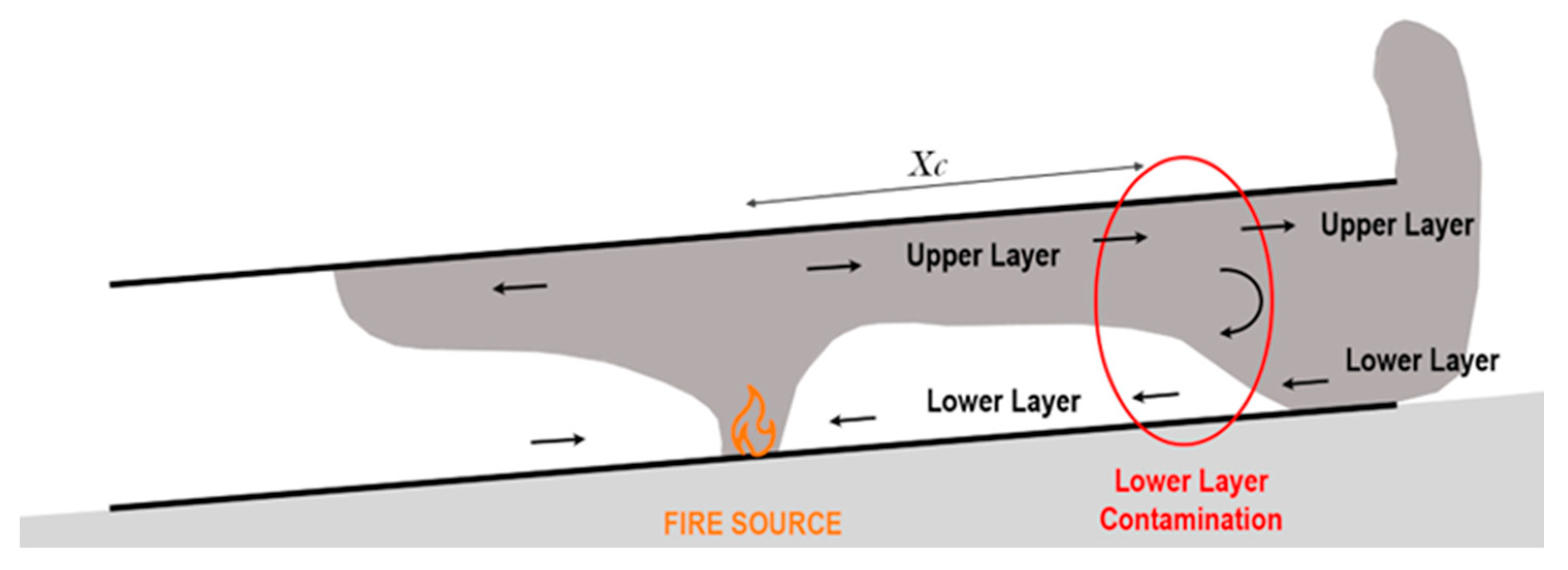
Directive 2004/54/EC [1] on minimum safety requirements for tunnels in the Trans-European Road Network is applicable to tunnels with lengths over 500 m. This Directive states that “mechanical ventilation systems shall be installed in all tunnels longer than 1000 m with a traffic volume higher than 2000 vehicles per lane”. This clause allows for avoiding the use of mechanical smoke control systems in shorter tunnels if the designer can prove that it is safe. In a horizontal tunnel, the flow from a fire source is symmetrical, and the smoke forms a hot upper layer flowing from the fire plume to the tunnel portals, while a cold lower layer of outside air flows from the portals and feeds the fire plume with fresh air. It is well known that the contamination of the cold lower layer with the smoke from the hot upper layer starts at some distance from the fire source, and the contaminated region increases as the smoke flows to the portals (Figure 1). The cold lower layer flow transports the smoke to the fire, and any smoke-free zone, subsisting from the beginning in the lower layer near the fire, will eventually be fully contaminated by the smoke. In this situation, people staying in this temporarily smoke-free zone will be trapped by the smoke and might not survive. If the distance from the fire to the tunnel portal is smaller than the distance to the point where the cold layer contamination starts, the cold layer remains clean and safe for users’ egress. Thus, it is of utmost importance to assess the distance where the cold layer contamination with smoke starts, considering the fire and the tunnel characteristics, because it allows one to decide whether the tunnel must be protected by a mechanical ventilation smoke control system or if the passive ventilation is enough for tunnel fire safety. This decision is very important because the costs associated with the installation and exploration of a mechanical ventilation system are high.

The studies regarding the lower layer contamination by smoke have mainly focused on the buoyancy effect using the Richardson number. Contamination occurs when the Richardson number is lower than 0.8 [2]. However, the results presented by Hinkley [3] and Yang et al. [4] show that this parameter is not sufficient to describe the real contamination behavior. The main reason is that stratification tends to be lost as the flow evolves. Yang et al. [4] proposed three stratification regions based on the Richardson and Froude numbers.

Most of the studies concerned with naturally ventilated tunnels focus on horizontal tunnels, and little research has been carried out on sloped tunnels. However, most tunnels are sloped for geographical reasons, being relevant to study the smoke flow due to fires in those tunnels. In the case of fires in naturally ventilated horizontal tunnels, there are two main flows, namely, an upper layer flow that exits the tunnel and a lower layer flow that moves towards the fire, but above a certain slope, due to the stack effect, the air entering through the lower part of the tunnel changes the fire and the flow dynamics in terms of flame, temperature, velocity and smoke layer thickness.

Smoke contamination mechanisms have not been sufficiently studied for sloped tunnels. One of the major earlier contributions was presented by Atkinson and Wu [5], who studied the relation between the velocity and the backlayering and proposed an equation to calculate the critical velocity in sloped tunnels. Merci [6] reported that the fire in sloped tunnels induces an airflow from the lower part of the tunnel due to the stack effect, and the intensity of this phenomenon depends on the heat release rate (HRR), slope, tunnel length, wall roughness, ambient temperature, tunnel cross-section and fire position. Zhang et al. [7] numerically investigated the maximum temperature and smoke backlayering length in a sloped tunnel under natural ventilation. They found that the smoke backlayering length decreases with the increase of the tunnel slope (due to the increment of the stack effect). However, they reported that the fire source heat release rate and tunnel width have no significant effect on the smoke backlayering length.

Li et al. [8] studied the effects of the surface roughness of the tunnel wall, air velocity, dimensions of the underground tunnel and temperature difference between the air and the tunnel wall on the variation of the temperature along a sloped tunnel under natural ventilation and studied its impact on the pressure differences due to buoyancy, which they refer to as thermal pressure. They found that for the same tunnel length and air velocity, the thermal pressure increases as the slope increases. They also found that for the same tunnel length, the thermal pressure decreases as the air velocity increases.

Yang et al. [9] carried out a series of simulations and small-scale experiments trying to simulate and recreate the effect of opposing mechanical ventilation for sloped tunnels. Even though the purpose was to recreate mechanical ventilation, their study is useful in understanding the behavior of fire with opposing wind. The main conclusions point to the importance of the HRR, slope, activation time and strength of forced ventilation as the main factors in predicting the dominant driving mechanism (stack effect-buoyancy or forced ventilation).

In recent years, several authors have investigated the propagation of smoke in inclined tunnels [10,11,12,13,14]. Ji et al. [10] studied the effects of ambient pressure on smoke movement and temperature distribution in sloped tunnels. They simulated cases between 50 kPa and 100 kPa in a tunnel of 130 m in length, 10 m in width, 5 m in height and an HHR of 5 MW. They found differences in the stack effect of the fire, which affects the flow in terms of temperature, mass flow rate and velocity. The lowest pressures are only relevant for tunnels at high altitudes. In the 100 kPa simulations (corresponding to tunnels closer to sea level), they obtained an increment of the smoke mass flow rate, induced velocity and a decrease of the maximum temperature as the slope increases. A remarkable feature in their results is that for an ambient pressure of 100 kPa, the backlayer length decreases as the slope increases (there is no backlayer for a slope of 15%), and there is no lower layer for the first 30 m of the flow for the 10% and 15% cases, stressing the effect of the slope on this behavior.

Gao et al. [11] studied the effect of the longitudinal slope on smoke propagation and ceiling temperature in naturally ventilated tunnels. They used a fire source of 3 MW and a tunnel of 60 m for slopes of 0%, 5%, 10% and 15%. They showed the relation of the stack effect with the slope and how the airflow changes the flow behavior. They found that there was no smoke outflow at the lower portal for the 15% case, in contrast to the other slopes, but there was a backlayer. However, the results are not representative of most fire locations for common tunnels because the tunnel length was rather small, and the fire position was close to the lower exit.

Fan et al. [12] carried out numerical tests to investigate the smoke movement characteristics under the stack effect in a mine laneway fire. They showed that increasing either the length or the angle of the inclined laneway decreases the smoke backlayering and forces more mass flow rate of smoke flowing in the inclined laneway. This effect was observed by Kong et al. [13,14], who studied the effect of a 15 MW (HHR) fire in sloped tunnels using the Fire Dynamics Simulator (FDS) computer code. They carried out an analysis of the influence of the position of the fire on the flow velocity, temperature, visibility and backlayer [13] for slopes from 0 to 10% in a tunnel of 500 m. The results were similar to the ones obtained by Gao et al. [11], but the tunnel considered by Kong et al. [13,14] was longer. In these studies, it was shown that there is no backlayer for slopes equal to or greater than 8.5%, which differs from the results presented by Gao et al. [11], where a slope of 15% still presents a backlayer; the cross-section, the tunnel length and the HRR were different, showing a stronger stack effect in the work of Kong et al. [13,14].

Recently, Wang et al. [15] carried out a small-scale experiment to investigate the influence of the slope on the backlayer for slopes of 4–35%. They observed a reduction of the backlayer depending on the slope, but a backlayer was still present for the slope of 35%. Caliendo et al. [16] carried out computational fluid dynamics (CFD) simulations considering the effects of the longitudinal slope on the risk level of users in naturally ventilated unidirectional road tunnels in the event of a fire accident. They found that the number of dangerous scenarios for user safety increased with adverse wind and/or negative gradients (i.e., vehicles circulating in the downhill direction).

Although the previous works represent an effort to increase the knowledge of the smoke flow due to a fire in sloped tunnels, just a few works give insight into the contamination of the lower layer with smoke. Galhardo et al. [17] showed that, for a horizontal tunnel, the upper layer mass flow rate grows when moving away from the fire (while the upper layer velocity magnitude is higher than the lower layer velocity magnitude) and reaches its maximum when both velocity magnitudes are equal. Further away from the fire, the hot upper layer is entrained by the cold layer flow, the mass flow rate of the hot upper layer decreases, and the lower layer contamination starts. Other authors, such as Hinkley [3], proposed that the lack of space to let the smoke cloud flow caused this type of mixing. However, these contributions are only relevant for horizontal tunnels, and the mechanisms generating the contamination of the lower layer with smoke are not clear for sloped tunnels. Thus, systematic research of the processes that cause the lower layer smoke contamination in sloped tunnels has never been made, and it is the purpose of the research presented in this article.

In a previous study [17], the authors studied the influence of wind velocity on the distance between the fire source and the beginning of the contamination of the lower layer with smoke for a horizontal tunnel. In this research, the objective is to explain the influence of the slope on that distance. This paper presents the research results in tunnels with a slope of 1% to 5% and shows how several relevant quantities (upper layer temperature, average mass flow rate, upper layer mass flow rate, upper layer velocity in the vicinity of the fire and lower layer velocity) depend on the physical processes that occur in the flow inside the tunnel using one-dimensional conservation equations found in the literature. It also shows that it is possible to use such equations to develop a one-dimensional model. The development of such a 1D model is relevant to allow a fast estimation of the point where the lower layer contamination with smoke starts. However, it is not expected that this estimation is as accurate as that determined from the CFD simulations.

2. Numerical Simulations

This study is based on CFD simulations using the FireFOAM software package (version 1912). This code uses the finite-volume method with second-order accuracy and implicit time integration. The pressure-implicit with splitting of operators (PISO) algorithm was used to numerically solve the pressure-velocity coupling. Turbulence was modelled using large-eddy simulation (LES). The radiation model assumed a gray medium with negligible scattering, and the finite-volume/discrete ordinates method was used. Combustion was modelled using the eddy dissipation model and assuming a global, mixing-controlled, irreversible reaction, considering the stoichiometric burning of dodecane with a fixed yield of soot (ν_soot = 0.038 g_soot/g_mixt). In the near-wall cells, wall functions were applied to predict the turbulent viscosity and the turbulent thermal diffusivity.

The fire source was modelled as a rectangular region whose upper surface is maintained at the boiling temperature of the fuel and at which the fuel velocity is prescribed according to the HRR. A no-slip condition for velocity was applied to the walls, assuming a wall roughness of 5 mm. The wall was assumed to behave as a semi-infinite solid with the properties of medium-weight concrete blocks exposed to convection and radiation. The estimated heat transfer coefficient was U_wall = 35 W·m⁻²·K⁻¹. The ambient temperature was T_∞ = 286 K (corresponding to the validation case). Additional details of the mathematical/physical formulation may be found in Galhardo et al. [17].

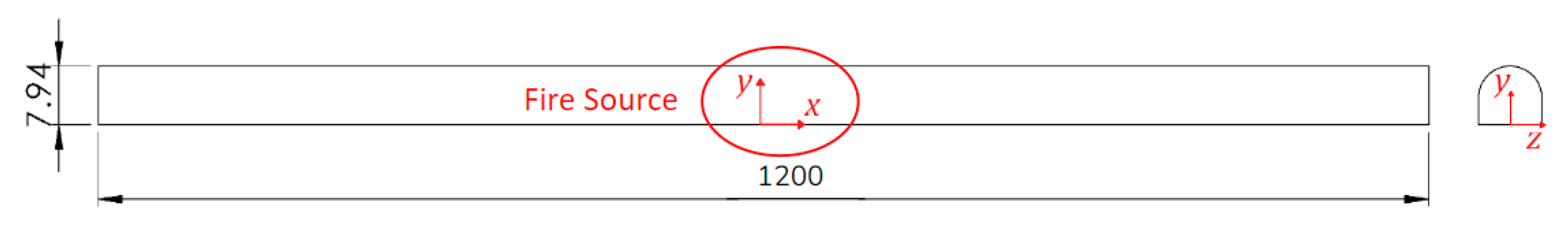
This work continues the research presented by Galhardo et al. [17]. In order to keep the results comparable, we used the same CFD code (FireFoam), the same case study (except that, in the present work, the tunnel is sloped and the length is 1200 m, see Figure 2), the same mesh and the same HRR. The use of the same case study allows us to consider the same validation and mesh refinement study. The mesh is refined in the vicinity of the fire source leading to three main regions (see Figure 3):

(a)

Region III: Thermal plume region, grid size Δ = 0.08 m.

(b)

Region II: Transition region between the thermal plume region and the region away from the fire, grid size Δ = 0.16 m.

(c)

Region I: Region away from the fire, grid size Δ = 0.32 m.

Figure 2. Dimensions [m] of the tunnel and reference frame centered at the fire source. The width of the tunnel is 8.56 m.

Figure 2. Dimensions [m] of the tunnel and reference frame centered at the fire source. The width of the tunnel is 8.56 m.

Figure 3. Mesh refinement in the vicinity of the fire source, which is represented by the white rectangle in Region III.

Figure 3. Mesh refinement in the vicinity of the fire source, which is represented by the white rectangle in Region III.

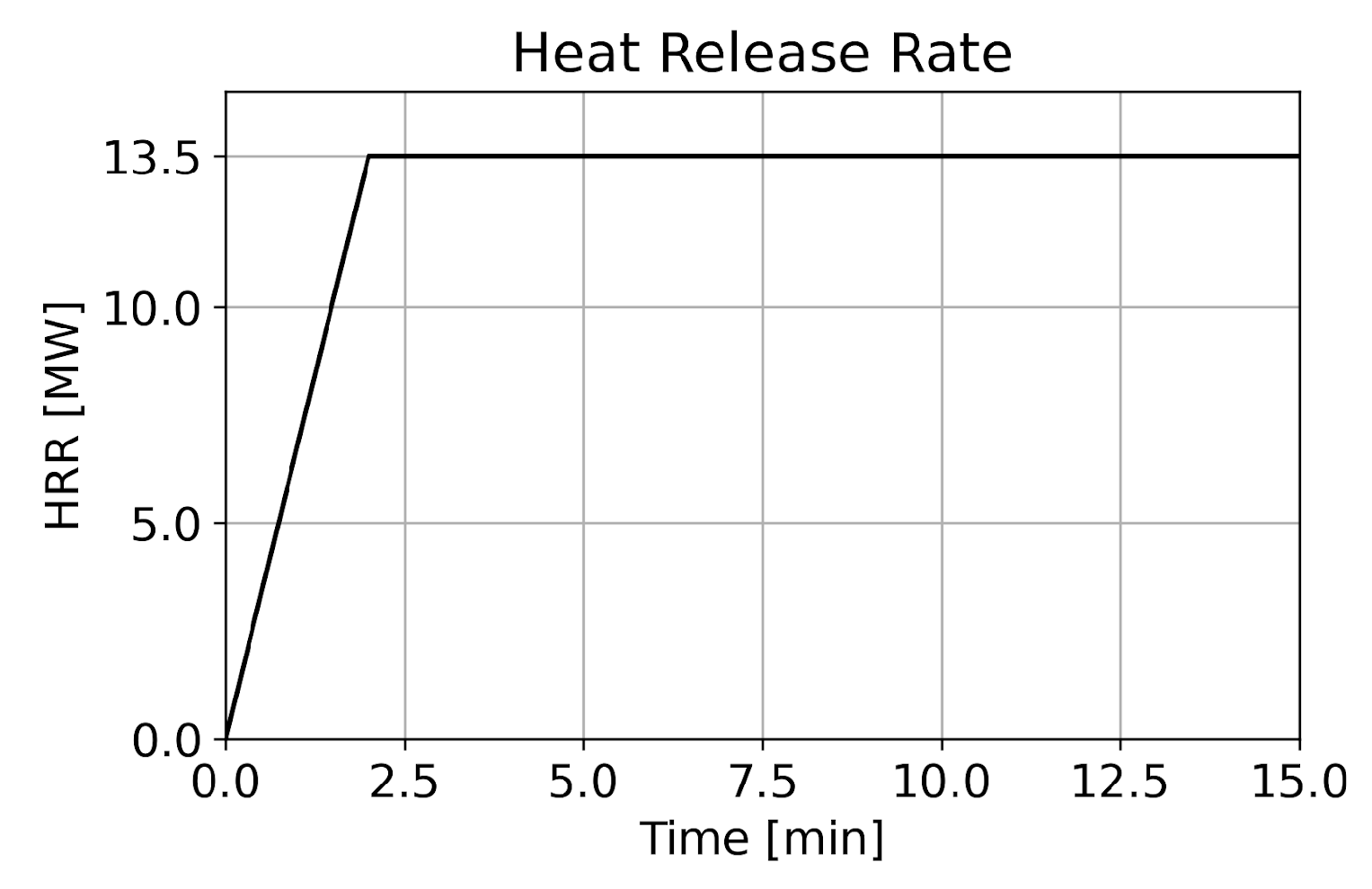
The CFD results were formerly validated [17] using the experimental results of the Memorial Tunnel Fire Ventilation Test Program [18]. The experiment consisted of a natural ventilated fire in a tunnel with a length of 853 m, slope of 3.2% and a horseshoe cross-section with a maximum width of 8.56 m, maximum height of 7.94 m and ambient temperature of 286 K. A diesel fuel known as fuel oil No. 2, which was modelled as dodecane (heat of combustion of dodecane = 47.8 MJ/kg), was used in the experiment. The fire source had a nominal power of 20 MW, but the measurements revealed that the HRR had an average value of 13.5 MW for over 16 min. The fire was located at a distance of 238 m from the south portal. The purpose was to consider a constant HRR in these simulations. 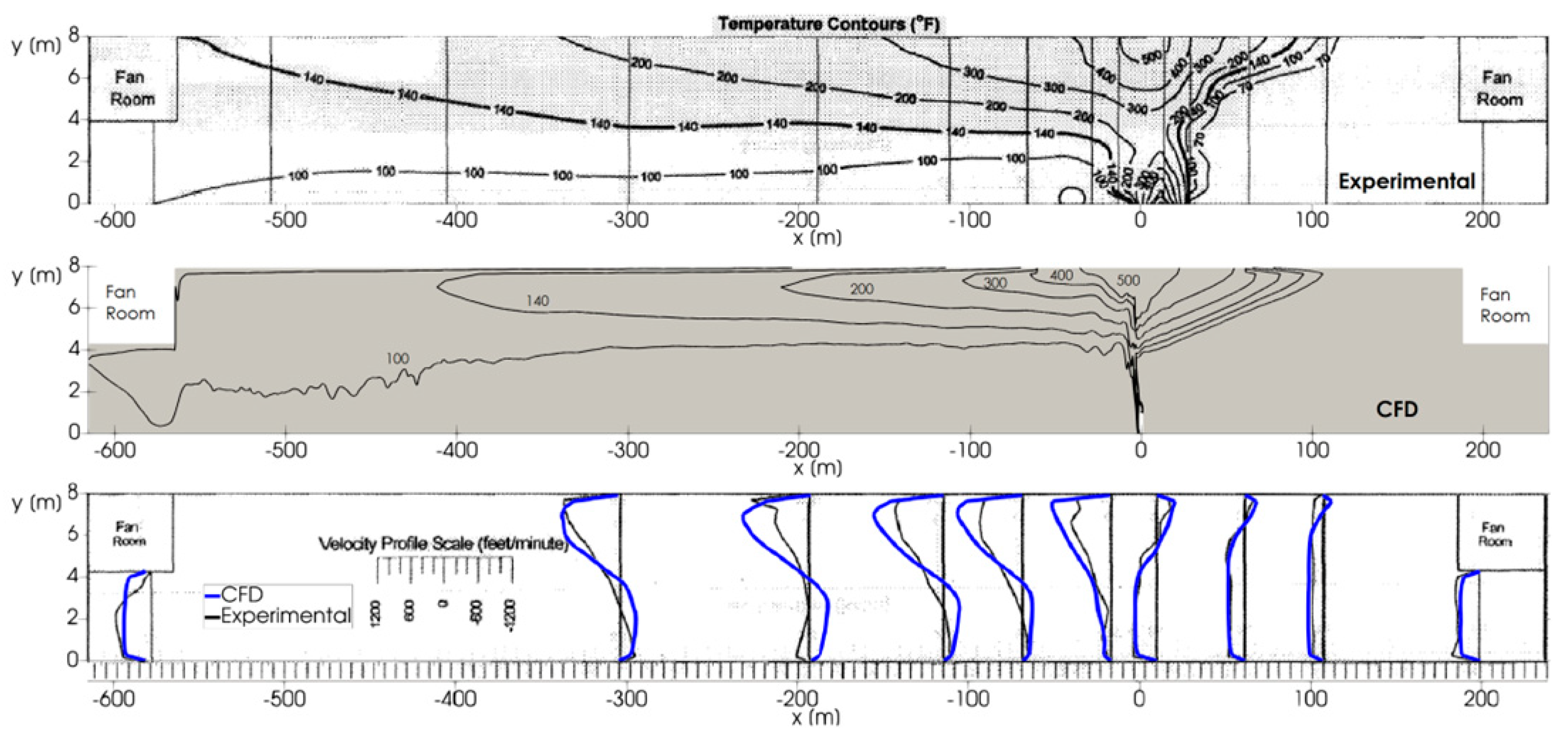In the CFD simulations, the HRR was 13.5 MW, the heat source area was 9.0 m² (the energy release density is 1.5 MW/m²) and the evolution can be seen in Figure 4. The initial transient increment of the HRR was adopted to avoid numerical instabilities. The comparison between the experimental and the simulation results at 2 min and 16 min after the full pan engulfment are presented in Figure 5 and Figure 6. Some discrepancies between the experimental and numerical temperature fields were found near the fire source at low heights. It is believed that this may be largely due to the lack of experimental data, which is only available at the vertical lines shown in Figure 5 and Figure 6 (top figure). The experimental temperature contours are plotted using such data, and the required interpolations between those lines may yield significant errors in regions of large gradients, such as in the vicinity of the fire source. The temperature predictions agree much more closely with the measurements in the ceiling jets. However, on the left side, the ceiling jet temperature is underpredicted. The simplifications inherent to the assumptions underlying the physical models used in the CFD predictions, the uncertainty of some input parameters of the CFD model (namely, the thermal properties of the walls and the average soot yield of the fuel, wind velocity and direction), errors in the measurements, caused by the influence of radiation on the thermocouples, and the approximations made in the modelling of the fire source are other reasons for the observed discrepancies. Furthermore, the comparison between the experimental and numerical velocity profiles shows that the CFD model is capable of yielding reasonable predictions of the longitudinal velocity field. In general, the CFD model has proven to be effective in simulating the large-scale behavior of the ceiling jet in this tunnel fire.

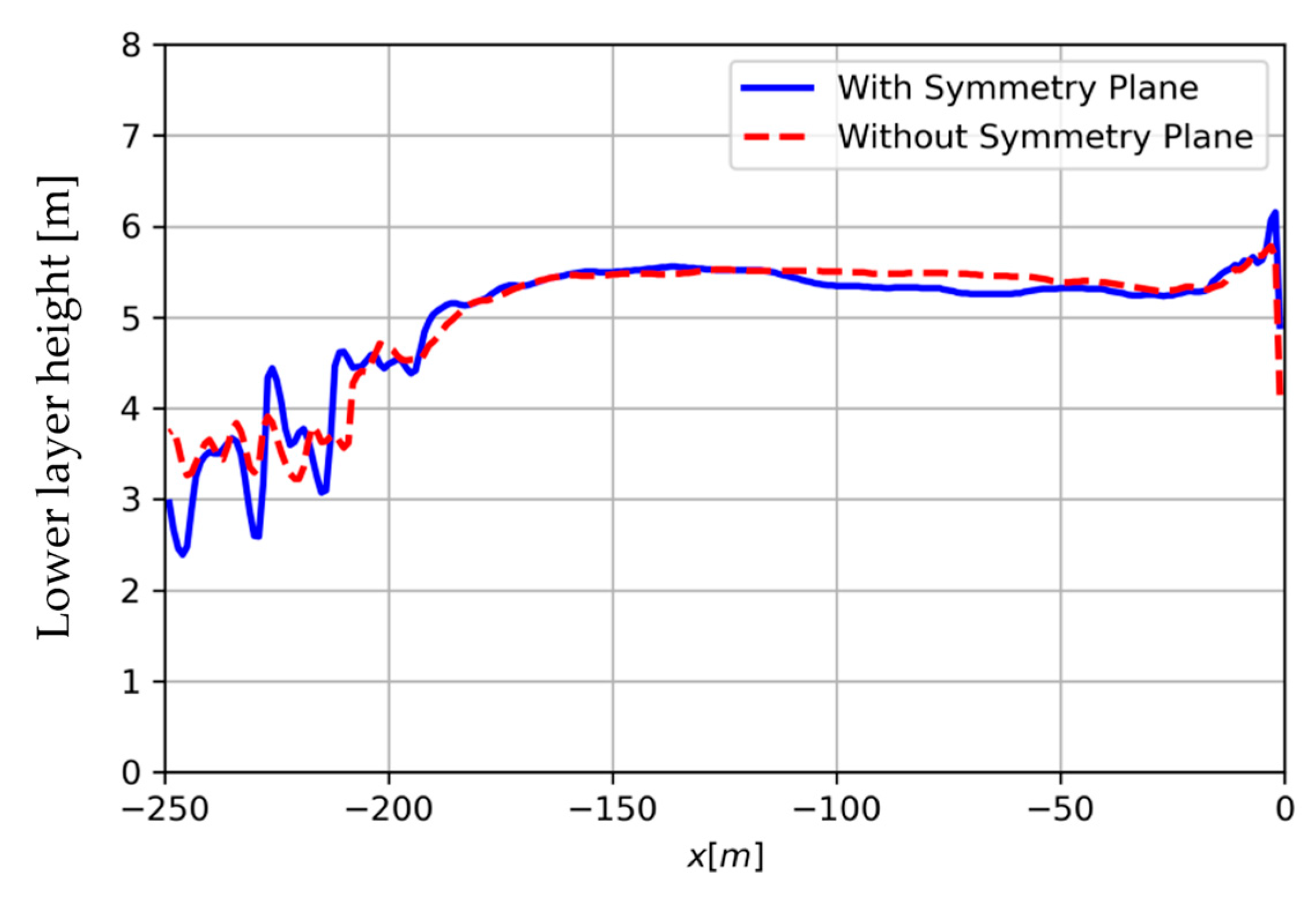
In the simulations, the quality of the mesh near the fire plume was assessed using the plume resolution index (PRI) [2], and it was found that PRI = 34, which is a sufficiently high value to accurately resolve the plume [17]. A mesh refinement study (carried out in the validation case to allow the comparison with test results) and an analysis to confirm that assuming symmetry is a good approximation were also carried out (see Figure 7). Further details can be found in Galhardo et al. [17].

After the validation, Galhardo et al. [17] studied several cases to assess the effect of the wind in horizontal naturally ventilated fire tunnels and its impact on the distance from the fire source to the location where the contamination of the lower layer with smoke starts. Our study is focused on the effect of the tunnel slope on that distance. CFD simulations for slopes ranging from 0.5% to 7.0% were carried out, excluding the wind action and considering only natural ventilation. The gravity vector was inclined to simulate the slope of the tunnel. An additional simulation for a slope of 2.0% was carried out considering an external wind velocity of 2.04 m/s blowing from the upper portal to the lower one. In Lisbon, the probability that the wind velocity exceeds this value is 0.3.

The length of the simulated tunnel was set to 1200 m, with the fire source centered, so that the portals do not influence the lower layer smoke contamination process. The conclusions of this research are applicable to shorter tunnels since the portals are far enough from the fire to avoid any significant influence on the contamination process.

In the simulations, no traffic was considered inside the tunnel, similar to most recent studies. The effect of the stopped cars, buses or trucks inside the tunnel, besides local generation of recirculating flows, would be the reduction of the average flow velocity. Since the prediction of the number of vehicles stopped inside the tunnel depends on the traffic of a specific tunnel, this research was carried out without stopping traffic.

3. Results of the CFD Simulations

Every simulation was run until a quasi-steady state was reached.

Table 1. Relevant times and mass flow rates.

Case	Slope (%)	Time to Exit the Tunnel (min)	Upper Layer Mass Flow Rate Peak Position (m)	Time to Achieve Steady State (min)	Average Mass Flow Rate (kg/s)
A	0.5	9	310	27	25.6 ± 0.6
B	1.0	8	230	18	37.2 ± 0.6
C	2.0	7	300	18	60.0 ± 0.2
D	3.5	6	210	13	73.4 ± 0.8
E	5.0	6	270	11	94.1 ± 0.6
F	7.0	5	20	11	130.3 ± 1.0

presents the results obtained in the simulations for slopes ranging from 0.5% to 7.0% concerning the time required for the smoke to reach the right tunnel portal (representing the exit of the tunnel), the distance from the fire source to the position of the maximum mass flow rate in the upper layer, the time to reach steady state flow (the steady state of the soot concentration field is reached later) and the mass flow rate once steady state is reached. The latter is invariant in the tunnel because it behaves similarly to a pipe with openings just at the ends.

Table 2. Maximum temperatures and velocities at the upper and lower layers.

Slope (%)	max(Tu(x)) [K]	max(Tl(x)) [K]	max(vu(x)) [m/s]	max(vl(x)) [m/s]
0.5	467	294	2.0	0.9
1.0	408	293	2.2	0.9
2.0	398	290	2.6	1.0
3.5	401	288	3.1	1.0
5.0	394	287	3.5	0.6
7.0	365	287	2.9	0.4

gives the maximum temperature, T, and velocity, v, at the upper (subscript u) and lower (subscript l) layers.

The average temperature and velocity at every cross-section of the tunnel were calculated for the upper and lower layers. The lower limit of the upper layer, which is coincident with the upper limit of the lower layer, is the surface where the flow velocity is equal to zero (v = 0). The direction of the flow in the upper layer is from the fire to the portal, and in the lower layer, it is from the portal to the fire. The mass flow rate is obtained by the integration of the mass flux (product of the density by the velocity component in the x-direction) over the cross-section of the tunnel. Similarly, the upper layer mass flow rate is obtained by integration over the region of the cross-section limited by the ceiling and the surface where v = 0, while the lower layer mass flow rate is computed similarly but for the region between the floor and the surface where v = 0.

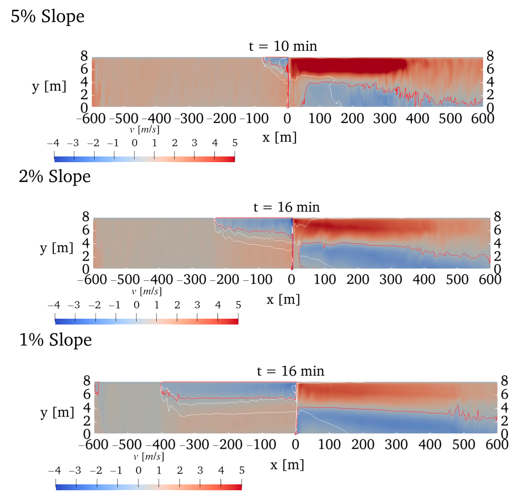
Figure 8 shows the predicted velocity magnitude, soot concentration and temperature contours at the longitudinal vertical symmetry plane for simulation C (2.0% of slope) and from 2 to 16 min after the beginning of the fire (the last time represents the steady state velocity field). Figure 9 shows the steady state contours for simulations A to F. The right portal is the highest one. The red line corresponds to the isovelocity line for v = 0, which separates the upper and the lower layers. The white lines represent a soot concentration of 300 mg/m³ (upper line) and 80 mg/m³ (lower line). The black lines correspond to temperatures of 27 °C and 127 °C, respectively. It is important to note that the results shown in Figure 8 and Figure 9 include both sides of the tunnel, while the tables and next figures (except Table 7 and Figures 14 and 17) only consider the highest part of the tunnel (from the fire source up to the right portal).

It can be observed in Figure 9 that the slope changes the behavior of the flow due to the buoyancy action. In a horizontal tunnel, the flow is symmetrical relative to the fire source, and there is a lower layer on both sides of the tunnel driving the outside cold air to the fire, as well as a hot upper layer driving out the smoke. In a sloped tunnel, the stack effect generates an airflow that enters through the lower part of the tunnel and the mass flow rate increases when the slope of the tunnel increases.

Three types of behavior were observed (see Figure 9):

(a)

Quasi-horizontal tunnel behavior (type 1): This behavior was observed in case A, which is the most similar to a horizontal tunnel. In the case of this small slope of 0.5%, the smoke may exit the tunnel from both portals (if the tunnel is short enough) because of the small contribution of the stack effect. Although the smoke layer on the left side of the fire source is not reaching the left portal in case A, it is clear that if the distance between the fire source and the left portal were lower than 500 m, the smoke could flow through the left portal. In the lower part of the tunnel (left side in the figures), the velocity of the cold air entering through the left portal is not sufficient to stop the upper layer flow.

(b)

Transitional behavior (type 2): This behavior was observed in cases B, C, D and E. In these cases, in the lower part of the tunnel, the velocity of the airflow entering through the left portal is higher than the upper layer velocity, thereby retaining the smoke and forming a backlayer. This behavior depends on the distance between the fire source and the lower portal (left portal in these cases) because if this distance is short, the backlayer may still reach the lower portal. 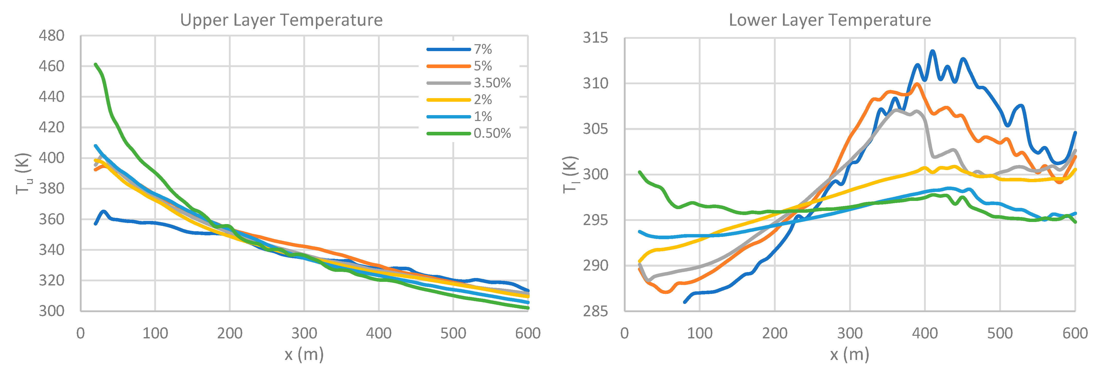As the slope increases, the upper layer velocity (see Table 2 and Figure 10) and the mass flow rate (see Table 1 and Figure 11) increase, the upper layer temperature decreases (Table 2 and Figure 12) and the backlayer shrinks. The upper layer temperature drop is caused by the energy losses due to heat transfer to the surroundings (walls, ceiling and floor) and the heat transferred to the mass flow of fluid in the lower layer, which increases with the slope. The increase in the slope of the tunnel leads to a decrease in the stability of the interface between the upper and lower layers in the upper part of the tunnel (right side in the figures), as revealed by the greater oscillations of the v = 0 isovelocity line.

(c)

Quasi-forced ventilation behavior (type 3): This behavior was observed in case F. There is no lower layer in some regions of the upper part of the tunnel (right side of the fire source), namely in the region close to the upper portal, where the velocity is positive at all heights, as illustrated in Figure 9, and so the lower layer does not reach that portal. The average upper layer velocity (Table 2 and Figure 10) decreases in case F in comparison to case E because the average lower layer velocity is smaller and has an opposite sign. Moreover, the area of the cross-section occupied by the lower layer is also smaller. The mass flow rate of the lower layer near the upper portal is close to zero (Figure 11). The velocity of the air entering through the left portal in the lower part of the tunnel almost equals the critical velocity needed to avoid the backlayer (see velocity contours in Figure 9).

Figure 10. Average upper (left) and lower (right) layers velocity from the fire to the upper portal for simulations A to F.

Figure 10. Average upper (left) and lower (right) layers velocity from the fire to the upper portal for simulations A to F.

Figure 11. Average upper (left) and lower (right) layers mass flow rate from the fire to the upper portal for simulations A to F.

Figure 11. Average upper (left) and lower (right) layers mass flow rate from the fire to the upper portal for simulations A to F.

Figure 12. Average upper (left) and lower (right) layers temperature from the fire to the upper portal for simulations A to F.

Figure 12. Average upper (left) and lower (right) layers temperature from the fire to the upper portal for simulations A to F.

Three main factors influence the velocity at the upper and lower layers: (i) buoyancy, (ii) mass flow entrainment and (iii) friction losses. In quasi-horizontal tunnels (type 1), the behavior of the upper and lower layers at both sides of the tunnel is similar to that observed in a horizontal tunnel in terms of entrainment mass flow and heat loss. The main difference is the effect of buoyancy that causes most of the smoke to exit through the upper part of the tunnel for a slope of 0.5%. In the case of tunnels with a slope ranging from 1% to 5% (type 2), the effects of buoyancy and entrainment mass flow are critical for the flow. The upper layer velocity (see Figure 10) increases with the slope, and the mass flow entrainment increases, reaching a peak for the 5% simulation (Figure 11). In the region zone between 400 and 600 m, instability between the upper and lower layers is observed (see the oscillations at the interface v = 0 in Figure 9). When the slope of the tunnel exceeds 5% (type 3), the average velocity of the upper and lower layers decreases, compared to the simulation for a slope of 5% (see Figure 9 and Figure 10).

The contamination of the lower layer with smoke from the upper layer depends on the slope of the tunnel. As the slope increases, the contamination occurs, in general, closer to the fire (see “Mass flow rate peak position” in Table 1). In case A (type 1), the contamination of the lower layer occurs on both sides of the fire, but the time span until the smoke exits the tunnel is the longest among the considered slopes (see Table 1). In cases B to E (type 2), the contamination only exists in the upper part of the tunnel (right side of the fire) and the time until the beginning of the contamination depends on the slope. In case F (type 3), the contamination only exists in the upper part of the tunnel, and the time until the beginning of the contamination is the shortest one among the studied cases.

Figure 13 shows that the mass flow rate at the upper layer is closely related to the difference between the average velocity at the upper and lower layers. This shows that the increment of the mass flow rate up to its peak (about 300 m from the fire source) is due to the mass entrainment from the lower layer. The decrease of the mass flow rate after the peak (as the distance from the fire source increases beyond 300 m) corresponds to the decay of the velocity difference between the two layers, which is related to the reduction of the thickness of the lower layer and the mass transfer to the lower layer.

Figure 8 shows that for a slope of 2%, the smoke contaminating the lower layer is stratified while it is hotter than the lower layer temperature. However, while the upper layer smoke is flowing to the portal, the smoke diffuses and dilutes into the lower layer. When the smoke transported by the lower layer flow approaches the fire source, its temperature becomes similar to the lower layer temperature, and the thermal stratification tends to be lost. This lower layer contaminated flow that approaches the fire source is very dangerous for tunnel users because it transports smoke into the occupation zone, where the users move and breathe. The lower layer contamination process is similar from 0% to 7% slope. The concentration of the combustion products depends on time (among other variables). Therefore, the users that are trapped by the lower layer contamination with smoke have a limited time to escape. Figure 9 shows that the time available to escape decreases when the slope increases.

A previous work [17] has shown that the external wind has an influence on the natural flow inside a horizontal tunnel. The opposing wind effect may significantly reduce the distance between the fire and the beginning of the lower layer contamination with smoke. An additional simulation, corresponding to the tunnel with a slope of 2.0% with descending wind action with an external velocity of 2.04 m/s, was carried out. Figure 14 compares the velocity field obtained with and without wind action. While in the corresponding case presented by Galhardo et al. [17], the distance between the fire source and the beginning of the lower layer contamination with smoke is reduced by 40%, in the sloped tunnel, there is just a slight difference between the cases with and without wind in the transient phase (see the plots corresponding to 7 min in Figure 14), and there is no significant difference between these two cases when steady state is reached.

4. Discussion

The CFD predictions of the evolution of several relevant quantities that control the smoke propagation and contamination in tunnel fires (upper layer temperature, mass flow rate, upper layer mass flow rate, upper layer average velocity in the vicinity of the fire and lower layer average velocity) are compared below with the results obtained from algebraic equations available in the literature. The input data for these equations are obtained from the CFD simulations. This analysis, which is aimed at a deeper understanding of the flow characteristics in sloped tunnels, stresses the physical processes relevant for the lower layer smoke contamination and supports the development of a one-dimensional (1D) model to predict the distance from the fire source to the location where the contamination of the lower layer with smoke starts. Although the same set of algebraic equations is used in this 1D model, the input data does not depend on the CFD results. This discussion is centered on the transitional regime (slope of 1% to 5%).

4.1. Upper Layer Temperature

The upper layer temperature averaged over a cross-section, $T_u$, in a fire tunnel may be predicted using the following equations [19]:

$$T_u=T_{\infty }+\left(T_{u max}-T_{\infty }\right)e^{-\frac{x}{x_e}}$$

(1)

$$x_e=\frac{{\rho }_{\infty }{\overline{C}}_p{\overline{v}}_{\infty }}{4h }\times D_H$$

(2)

where $T_{\infty }$ is the external air temperature, $T_{u max}$ is the maximum upper layer temperature, x is the tunnel longitudinal coordinate, ${\overline{C}}_p$ is the specific heat of the smoke calculated at the average temperature between $T_{\infty }$ and $T_{u max}$, ${\rho }_{\infty }$ is the external air density, ${\overline{v}}_{\infty }$ is the average flow velocity inside the tunnel at the temperature $T_{\infty }$ and $D_H$ is the hydraulic diameter of the cross-section of the tunnel. The variable $h$ is the heat exchange coefficient between the smoke and the inner surfaces of the tunnel (tunnel walls and ceiling), which is estimated as follows:

$$h=\frac{{\phi }_c+{\phi }_r}{T_u-T_{\infty }}$$

(3)

where ${\phi }_c$ is the convective heat flux and ${\phi }_r$ is the radiative heat flux. These fluxes are predicted by Equations (4) and (5).

$${\phi }_r=\epsilon \sigma F\left(T_u^4-T_p^4\right)$$

(4)

$${\phi }_c=h_c\left(T_u-T_p\right)$$

(5)

where $\epsilon$ is the surface emissivity, $\sigma$ is the Stefan–Boltzmann constant, $F$ is a shape factor ($F\approx 1$), $T_p$ is the inner surface temperature (the wall and ceiling are at ambient temperature in the beginning of the fire) and h_c is the convective heat transfer coefficient, which may be estimated from the following correlation [19]:

$$h_c=\frac{\left(\frac{f}{8}\right){\overline{C}}_p\rho v}{1.07+12\left(P{r}^{2/3}-1\right)\sqrt{\frac{f}{8}} }$$

(6)

where $Pr$ is the Prandtl Number, $v$ is the average flow velocity over the cross-section and $f$ is the tunnel wall friction factor.

The maximum temperature at 10 mm below the ceiling for the transitional behavior is obtained using the following equations presented by Huo et al. [20]:

$${\dot{Q}}^{*}{}_c=\frac{0.7\dot{Q}}{{\rho }_{\infty }{\overline{C}}_p{T}_{\infty }\sqrt{g}{H}^{\frac{5}{2}} }$$

(7)

$$\frac{\frac{\Delta T}{T_{\infty }}}{{\dot{(Q}}^{*}{}_{c}cos\theta ){ }^{\frac{2}{3}}}={\left(0.188+0.313\frac{r_{up}cos\theta }{H}\right)}^{-\frac{4}{3}}$$

(8)

where $\dot{Q}$ is the heat release rate, $r_{up}$ is the radial distance of the ceiling jet from the plume-impingement point to the upper tunnel opening, H is the ceiling height above the fire source, $\theta$ is the slope angle and ΔT = T_max − T_∞. Equation (8) yields, for $r_{up}=0$,

$$T_{max}=T_{\infty }{\left({\dot{Q}}_c^{*}cos\theta \right)}^{\frac{2}{3}}{\left(0.188\right)}^{-\frac{4}{3}}+T_{\infty }$$

(9)

Using the data for the upper layer at the upper part of the tunnel and taking $T_{u max}$ in Equation (1) equal to $T_{max}$ given by Equation (10), the results calculated from the above equations are presented in

Table 3. Results of the heat transfer equations.

Slope (%)	${\mathit{\phi }}_{\mathit{c}} (\mathbf{W}/{\mathbf{m}}^2)$	${\mathit{\phi }}_{\mathit{r}} (\mathbf{W}/{\mathbf{m}}^2)$	$\mathit{h} \left(\mathbf{W}\mathbf{·}{\mathbf{m}}^{-2}\mathbf{·}{\mathbf{K}}^{-1}\right)$	${\mathit{x}}_{\mathit{e}} \left(\mathbf{m}\right)$	${\mathit{T}}_{\mathit{m}\mathit{a}\mathit{x}} \left(\mathbf{K}\right)$
1.0	141.5	174.2	7.2	232.0	747.8
2.0	146.5	155.8	7.1	294.8	747.7
3.5	203.3	173.1	8.1	248.2	747.6
5.0	160.0	134.8	7.0	422.9	747.4

. Using the least squares method to fit Equation (1) to the CFD simulation results, the best fit for the variables $T_{u max,CFD}$ and $h_{CFD}$ is presented in

Table 4. Results of the heat transfer equations.

Slope (%)	Tu max,CFD (K)	${\mathit{h}}_{\mathit{C}\mathit{F}\mathit{D}} \left(\mathbf{W}\mathbf{·}{\mathbf{m}}^{-2}\mathbf{·}{\mathbf{K}}^{-1}\right)$	Tmax,eqs (K)	${\mathit{h}}_{\mathit{eqs}} \left(\mathbf{W}\mathbf{·}{\mathbf{m}}^{-2}\mathit{·}{\mathbf{K}}^{-1}\right)$	$\frac{{\mathit{T}}_{\mathit{u} \mathit{m}\mathit{a}\mathit{x},\mathit{C}\mathit{F}\mathit{D}}}{{\mathit{T}}_{\mathit{m}\mathit{a}\mathit{x},\mathit{e}\mathit{q}\mathit{s}}}$	$\frac{{\mathit{h}}_{\mathit{C}\mathit{F}\mathit{D}}}{{\mathit{h}}_{\mathit{e}\mathit{q}\mathit{s}}}$
1.0	410.7	5.1	747.8	7.2	0.53	0.71
2.0	399.6	5.7	747.7	7.1	0.53	0.80
3.5	402.0	7.5	747.6	8.1	0.54	0.99
5.0	402.1	7.5	747.4	7.0	0.54	1.07

. This table also presents the values $T_{max,eqs}$ and $h_{eqs}$ calculated from Equations (9) and (3)—subscript eqs is included here to distinguish from the CFD results.

Note that Equations (1) and (2) were developed for a horizontal tunnel but applied to an inclined one here. Moreover, $T_{max}$ is expected to be greater than $T_{u max}$ since the former is the temperature at 10 mm below the ceiling at the plume impingement point, while the latter is the maximum value of the upper layer temperature averaged over a cross-section, as stated above. Therefore, the discrepancies observed in Table 4 are not surprising. Hence, a polynomial function was derived in order to correct the values of $h_{eqs}$ and $T_{max,eqs}$ obtained from the algebraic Equations (3) and (9) in order to match the CFD results:

$$h_{eqs,corr}\left(\gamma \right)=h_{eqs}\left(0\right)\times \left(-0.0097{\gamma }^2+0.151\gamma +0.5578\right)$$

(10)

$$T_{max,eqs,corr}\left(\gamma \right)=T_{max,eqs}\left(0\right)\times \left(-0.0019{\gamma }^3+0.0194{\gamma }^2-0.0593\gamma +0.5911\right)$$

(11)

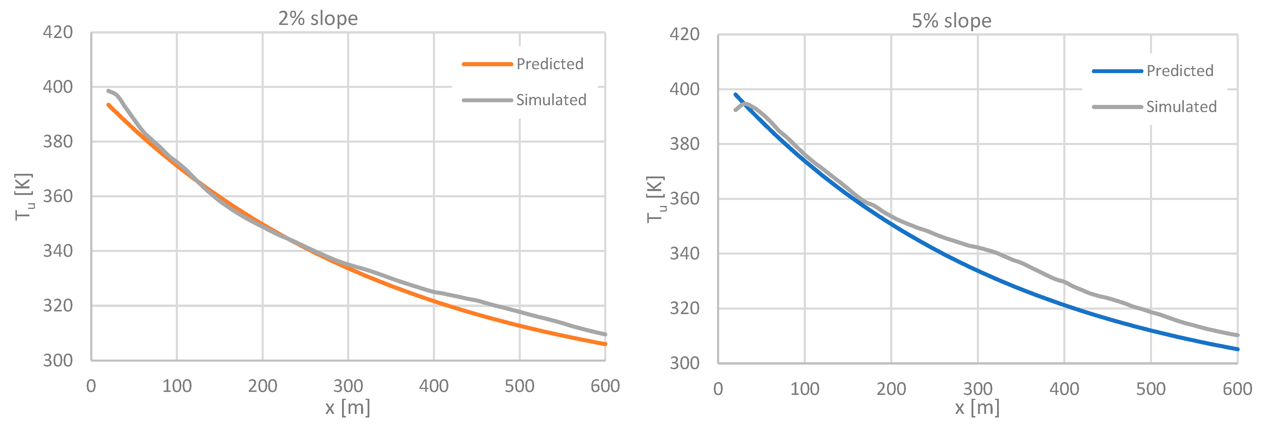
where $\gamma$ is the slope of the tunnel [%] and subscript corr denotes a corrected value. Figure 15 compares the upper layer temperature decay from the vicinity of the fire source to the upper portal obtained by the CFD simulations, with the temperature being predicted using Equations (1) to (6) and (9) to (11). The curves correspond to slopes of 2% and 5% and show a good agreement between the results of the CFD simulation and the heat transfer equations.

4.2. Average Mass Flow Rate

Another quantity that is relevant for this analysis is the mass flow rate in the tunnel. As the tunnel has openings (portals) at both ends, the mass flow rate must be uniform along the tunnel when steady-state conditions are reached, according to the continuity equation. Table 1 shows that the mass flow rate increases with the slope, being related to the increment of the stack effect. The one-dimensional flow model proposed by CETU [19] is used in the form presented by Viegas et al. [21] to explain this trend, which yields

$$\gamma {\rho }_{\infty }\left(1-\frac{T_{\infty }}{T_u}\right)gL=f{\rho }_{\infty }\frac{T_{\infty }{v}^2}{2T{D}_H}L+\frac{1}{2}\epsilon {\rho }_{\infty }\frac{T_{\infty }}{T_u}{v}^2+F\left({\dot{Q}}_c\right)$$

(12)

where g is the gravity acceleration, L is the length of the tunnel, v is the flow velocity averaged over a cross-section inside the tunnel and $\epsilon$ is the pressure loss coefficient. The term on the left side represents the stack effect, while the first term on the right side represents the pressure loss along the tunnel gallery; the second term accounts for the local pressure losses at the entrance and exit portals; and the third term, $F\left({\dot{Q}}_c\right),$ is the pressure loss that occurs at the fire site. Little research has been carried out on the pressure drop at the fire site. CETU [19] proposed Equation (13), based on CFD simulation results with the average flow velocity in the range of 1.5 m/s to 3.5 m/s, where the local pressure loss decreases when the average flow velocity increases:

$$F\left({\dot{Q}}_c\right)=9\times {10}^{-5}\frac{{\dot{Q}}_c}{v{D}_H^2}$$

(13)

A recent work carried out by Ang et al. [22] presents the following equation, also based on results from CFD simulations, where the local pressure loss increases when the average flow velocity increases:

$$F\left({\dot{Q}}_c\right)=\frac{3{\dot{Q}}_{c}v}{2S{T}_{\infty }{c}_p}$$

(14)

Due to the lack of agreement about how the average flow velocity influences the pressure loss in the local of the fire, a constant value was considered in the present work. The range of the average flow velocity of the cold flow (at the left-hand side of the fire source), which is required in both equations, is between 0.86 m/s (slope of 0.5%) and 3.13 m/s (slope of 5.0%). These velocities were estimated by Equation (12). In the range from 2.5 m/s to 3.13 m/s, the average pressure loss in the fire site computed from Equations (13) and (14) varies between 3.5 Pa and 3.2 Pa, while for lower velocities, there is a big increment of the pressure loss predicted by Equation (13) that is hardly compatible with the small stack effect generated for small slopes (e.g., the estimated stack effect for the slope of 0.5% is just 5.4 Pa). Therefore, the average pressure loss in the local of the fire was rounded to $F\left({\dot{Q}}_c\right)=3 \mathrm{Pa},$ and this constant value was adopted for the whole average flow velocity range.

The mass flow rate $\dot{M}$ is obtained from Equation (15), where $S$ is the area of the cross-section of the tunnel:

$$\dot{M}=Sv{\rho }_{}$$

(15)

The upper layer temperature averaged over a cross-section is obtained using the method presented by CETU [19], based on Equations (1) and (2), where $T_{u,max}$ was calculated using the following equation:

$$T_{max}=\frac{{\dot{Q}}_c}{{\rho }_{\infty }{\overline{C}}_{p}Sv}+T_{\infty }$$

(16)

The tunnel was discretized into sections with a length of 10 m, and T_u was assumed to be constant in each section. The density, ρ, and other temperature-dependent quantities are updated according to the local temperature, T_u. The following values, common for tunnels [19], have been considered: $h=8$.5 W/m²·K, f = 0.020, $\xi$ = 1.84. The density values (for the stack effect) are obtained considering the convective heat release rate of ${\dot{Q}}_c=13.5\times 0.7 \mathrm{MW}$.

In

Table 5. Analysis of the mass flow rate [kg/s].

Slope	${\dot{\mathit{M}}}_{\mathit{CFD}}$	${\dot{\mathit{M}}}_{\mathit{eq}.13}$	${\dot{\mathit{M}}}_{\mathit{C}\mathit{F}\mathit{D}}/{\dot{\mathit{M}}}_{\mathit{e}\mathit{q}.13}$	${\dot{\mathit{M}}}_{\mathit{eq}.13}\times {\left({\dot{\mathit{M}}}_{\mathit{C}\mathit{F}\mathit{D}}/{\dot{\mathit{M}}}_{\mathit{e}\mathit{q}.13}\right)}_{\mathit{a}\mathit{v}\mathit{e}\mathit{r}\mathit{a}\mathit{g}\mathit{e}}$
0.5%	26	50	0.55	25
1.0%	37	83	0.45	41
2.0%	60	120	0.50	59
3.5%	73	156	0.47	77
5.0%	94	182	0.52	90
Average			0.50

, the mass flow rate in the tunnel obtained in the CFD simulations with slopes from 0.5% to 5.0% and the mass flow rate predicted from Equation (15) are presented for steady state. The ratio of the values obtained from the CFD simulations to those predicted from Equation (15) ranges from 0.45 to 0.55, with the average value being 0.50. The last column in Table 5 presents the values obtained from the product of the mass flow rate calculated using Equation (15) by the average of the ratio of the CFD to Equation (15) predictions. This confirms that the mass flow rate in the tunnel is directly proportional to the stack effect. However, this simple pipe loss model just considers a one-dimensional flow in a pipe and the flow to the right side of the fire source is much more complex. It is expected that the friction losses on the right side of the tunnel are greater than those predicted by this one-dimensional model. According to these results, the overall losses are about twice the ones predicted by the above equations.

4.3. Upper Layer Mass Flow Rate

The results of the simulations show the increment of the mass flow rate at the upper layer with the increment of the distance to the fire source (see Figure 13), which is due to the entrainment of the lower layer. A previous work [17] showed that this entrainment obeys Equation (17) for a horizontal tunnel.

$$\Delta {\dot{M}}_u={\rho }_{\infty }W{C}_{\beta }R{i}^{-1}\left(v_u-v_l\right)\Delta x$$

(17)

$$Ri=\frac{\left({\rho }_{\infty }-{\rho }_u\right)g{h}_u}{{\rho }_u{\left(\left|v_u\right|+\left|v_l\right|\right)}^2}$$

(18)

where ${\dot{M}}_u$ is the upper layer mass flow rate, W is the width of the interface between the upper and lower layers, Ri is the Richardson number, $v_u$ and $v_l$ are the upper and lower layer average velocities, respectively, at the cross-section under consideration, ρ_u is the upper layer density, $h_u$ is the upper layer thickness and $C_{\beta }$ is a model constant related to the entrainment coefficient $\beta$. The value $C_{\beta }=0.0109$ obtained by Galhardo et al. [17] was used here.

Figure 16 compares the upper layer mass flow rate obtained from Equation (17) (denoted by “Pred1”), which overestimates the CFD results and fails to correctly predict the increase of the upper layer mass flow rate, and Equation (19) (denoted by “Pred2”), where the mass entrainment is linearly related to the shear layer velocity difference:

$$\Delta {\dot{M}}_u={\rho }_{\infty }W{C}_{\beta }\left(v_u-v_l\right)\Delta x$$

(19)

The value $C_{\beta }=0.004$, corresponding to the best fit for the four cases (slope from 1% to 5%), was used. This shows that the initial increment of the upper layer mass flow rate in sloped tunnels is close to a linear variation with the shear layer velocity difference.

Table 6. Mass flow rate in the CFD simulations [kg/s].

Slope	Upper Layer Peak	Upper Layer x = 20 m	Average
0.0%	26	16
0.5%	55	42	26
1.0%	66	50	37
2.0%	84	66	60
3.5%	94	78	73
5.0%	113	94	94

compares the peak mass flow rate, the mass flow rate and the upper layer mass flow rate at x = 20 m (20 m to the right of the fire) obtained in the CFD simulations. The values of the mass flow rate for slopes in the range of 2% to 5% are relatively close to the values of the upper layer mass flow rate at x = 20 m, while for slopes lower than 2%, the upper layer mass flow rate at x = 20 m is significantly higher than the average mass flow rate. Figure 17 compares the velocity field at the vertical symmetry plane for slopes of 1%, 2% and 5%. It shows that the plume rising from the heat source is dragged by the velocity due to the stack effect along the tunnel, which increases with the slope. At the cross-section x = 20 m and for a slope of 1%, the fluid in the lower layer flows from the right portal to the fire, while for a slope of 2% or higher, the fluid in the lower layer entering through the right portal does not reach the cross-section at x = 20 m. Therefore, in the latter case, the upper layer mass flow rate is close to the mass flow rate. This conclusion allows using the mass flow rate as the initial value of the upper layer mass flow rate.

4.4. Upper Layer Velocity in the Vicinity of the Fire

The assessment of the variation of the upper layer velocity is based on the momentum equation, which may be written as

$$\frac{d}{dx}\left(S_u{\rho }_u{v}_u^2\right)=S_u\left({\rho }_{\infty }-{\rho }_u\right)\gamma g-S_{u}f\frac{\rho v_u^2}{2D_{H u}}$$

(20)

where $S_u$ is the area of the cross-section of the upper layer and $D_{H u}$ is the upper layer hydraulic diameter. The left side of Equation (20) represents the rate of change of the momentum, while on the right side of the equation, the first term represents the momentum source due to buoyancy (in a sloped tunnel), and the second term represents the friction losses in the tunnel walls and ceiling.

Considering that when using the ideal gas law, the upper layer density may be expressed by Equation (21) and that the upper layer mass flow rate ${\dot{M}}_u=S_u{\rho }_u{v}_u$, then Equation (22) is obtained:

$${\rho }_u={\rho }_{\infty }\frac{T_{\infty }}{T_u}$$

(21)

$$\frac{d}{dx}\left({\dot{M}}_u{v}_u\right)={\rho }_{\infty }{S}_u\left(1-\frac{T_{\infty }}{T_u}\right)\gamma g-S_{u}f{\rho }_{\infty }\frac{T_{\infty }{v}_u^2}{2T_u{D}_{H u}}$$

(22)

Expanding the derivative term and considering that the velocity may be approximated by a piecewise linear profile, the momentum balance may be expressed as

$$v_u\Delta {\dot{M}}_u+{\dot{M}}_u\Delta v_u=S_u{\rho }_{\infty }\left(1-\frac{T_{\infty }}{T_u}\right)\gamma g\Delta x-S_{u}f{\rho }_{\infty }\frac{T_{\infty }{v}_u^2}{2T_u{D}_{H u}}\Delta x$$

(23)

In the case of a slopped tunnel, the upper layer mass flow rate is incremented due to the entrainment of cold air from the lower layer, as expressed by the following equation:

$$\frac{d}{dx}\left({\dot{M}}_u\right)=W{\rho }_{\infty }{v}_{entrain}$$

(24)

where W is the width of the tunnel and $v_{entrain}$ is the entrainment velocity given by

$$v_{entrain}=C_{\beta }\left(v_u-v_l\right)$$

(25)

yielding

$$\frac{d}{dx}\left({\dot{M}}_u\right)=W{\rho }_{\infty }{C}_{\beta }\left(v_u-v_l\right)$$

(26)

Equation (19) is obtained from Equation (26) by considering a piecewise linear velocity profile, which was shown above to be an acceptable approach for the upper layer mass flow rate increment phase.

Finally, Equation (23) may be rewritten as follows:

$$\Delta v_u=\frac{S_u{\rho }_{\infty }\left(1-\frac{T_{\infty }}{T_u}\right)\gamma cg-S_{u}f{\rho }_{\infty }\frac{T_{\infty }{v}_u^2}{2T_u{D}_{H u}}-v_{u}W{\rho }_{\infty }{C}_{\beta }\left(v_u-v_l\right)}{{\dot{M}}_u}\Delta x$$

(27)

In this equation, a proportionality constant “c” was introduced in the buoyancy term to allow weighting of this term when determining the best fit to the simulation results. The values of $S_u$, $T_u$, $v_u$, $v_l$ and ${\dot{M}}_u$ resulting from the CFD simulations were used in this equation, and $\Delta x$ was set to 20 m. The values of the initial velocity $v_u\left(0\right)$, $C_{\beta }$, $c$ and $f$ were found by the least squares fit of Equation (27), from 0 m to 400 m, to the upper layer velocity curve obtained from the CFD simulations (see

Table 7. Parameters of Equation (27) obtained by the least squares fit of Equation (27) to the results of the CFD simulations.

Slope	Initial Velocity [m/s]	${\mathit{C}}_{\mathit{\beta }}$	c	f (Friction Factor)
1.0%	1.26	0	0.50	0.024
2.0%	1.87	0	0.27	0.020
3.5%	1.31	0	0.39	0.035
5.0%	1.35	0	0.21	0.021
Average	1.45	0	0.34	0.025

) for every slope.

Figure 18 compares the steady state upper layer velocity curve obtained by CFD simulation (blue line) and from Equation (27) (denoted by “Pred”, the red line). Equation (27) allows a good approach for the simulated values of upper layer velocity up to about 400 m to the fire source, except for the slope of 5%. In the latter case, a good approach is obtained only up to about 200 m. The increase of the upper layer velocity as the distance from the fire increases is due to the buoyancy term, where the parameter “c” lies in the range of 0.21 to 0.50. The decrease of the upper layer velocity at a larger distance from the fire is due to the friction loss term. The friction factor lies in the range of 0.020 to 0.035. This factor also includes the friction losses in the shear layer between the upper and lower layers, which are not explicitly considered in Equation (27). Note that the value f = 0.020 is currently used in tunnels with concrete walls [19]. In these four cases, the influence of the term related to the upper layer mass flow rate increment is not relevant ($C_{\beta }=0$ in Table 7).

4.5. Lower Layer Velocity

The lower layer velocity may be estimated from the following mass balance:

$$\dot{M}={\dot{M}}_u-{\dot{M}}_l$$

(28)

where ${\dot{M}}_l$ is the average mass flow rate in the lower layer, which is given by

$${\dot{M}}_l=S_l{v}_l{\rho }_{\infty }$$

(29)

where $S_l$ is the area of the cross-section of the lower layer, yielding

$$\dot{M}={\dot{M}}_u-S_l{v}_l{\rho }_{\infty }$$

(30)

The lower layer velocity $v_l$ may be written as

$$v_l=\frac{{\dot{M}}_u-\dot{M}}{S_l{\rho }_{\infty }}$$

(31)

or

$$v_l=\frac{{\dot{M}}_u-\dot{M}}{{\rho }_{\infty }\left(S-S_u\right)}$$

(32)

Figure 19 shows the results obtained for $\Delta v=v_u-v_l$ (“u_dif_pred”), where $v_u$ was obtained from the CFD simulations and $v_l$ was calculated from Equation (32). The CFD simulation results for the difference $\Delta v=v_u-v_l$ are also presented in Figure 19 and show that the value of $v_l$ calculated from Equation (32) is very close to that obtained from the CFD simulations.

At the lower layer on the right side of the tunnel, the velocity is negative, i.e., the fluid flows from the right portal to the fire. This layer is due to the momentum generated by buoyancy in the fire plume and to the thermal stratification in the tunnel. Due to the friction losses in the tunnel, the effect of the momentum generated by the fire plume is more important near the fire, while far from the fire, the difference between the upper layer and lower layer velocities is mainly due to the pressure differences created by the higher temperature of the upper layer.

The maximum difference between the upper layer and lower layer velocities of the flow may be predicted as follows [23]:

$$\Delta v=\sqrt{2g\left(\frac{T_u}{T_{\infty }}-1\right)h_u}$$

(33)

where $h_u$ is the upper layer thickness. A similar equation, affected by a coefficient of 0.8, is applied to long corridors [3]. This equation may be seen as the maximum velocity difference allowed due to the temperature inside the tunnel (far from the fire plume influence). This value is presented in Figure 19 (“u_dif_max”), and it is clear that the CFD predictions of $\Delta v={\overline{v}}_u-{\overline{v}}_l$ are generally lower than those determined from Equation (33).

When the variation of the upper layer mass flow rate ${\dot{M}}_u,$ given by Equation (17), is considered in Equation (32), the value of the lower layer velocity $v_l$ necessary to balance the mass flow increases too much and crosses the line that shows the velocity difference given by Equation (32), meaning that it is not possible to have such a large velocity difference between the upper and lower layer (see Figure 20). It is due to this impossibility that the upper layer mass flow rate does not vary according to Equation (17) but rather according to Equation (19), as previously shown.

The intersection of the line determined from Equation (32), with ${\dot{M}}_u$ given by Equation (17), with the line given by Equation (33), represents a conservative approximation of the physical limit above which the mass flow rate of the upper layer cannot increase. Farther away from the fire source, due to the reduction of temperature, the velocity difference between the upper and the lower layers is reduced, and the mass flow rate of the upper layer must decrease, thereby starting the contamination of the lower layer. The value of the upper layer mass flow rate at x = 0 was set equal to the predicted mass flow rate given in Table 5.

In Figure 20, the upper layer mass flow rate is also presented (y-axis on the right side of the chart) to show that, although the intersection point mentioned above is not coincident with the peak of the mass flow rate, it is in the range of the plateau around this peak.

Table 8. Longitudinal coordinate x_c corresponding to the beginning of smoke contamination of the lower layer.

Slope	xc [m]
	CFD Simulation	Predicted (Ri)
1.0%	230	270
2.0%	300	240
3.5%	210	180
5.0%	270	200

shows the values of the longitudinal coordinate x_c obtained by the intersection of the line that represents the velocity difference given by Equation (32), considering that ${\dot{M}}_u$ is given by Equation (17), with the line given by Equation (33) [“Predicted (Ri)”]. It also shows x_c determined from the CFD simulations, which corresponds to the location of the peak of the upper layer mass flow rate. The predictions obtained from the algebraic equations deviate by 14% to 26% from the CFD predictions of x_c, depending on the slope of the tunnel. While the predictions show a general trend of decrease with the slope increment, the CFD results show a somewhat irregular behavior. This is due to the upper layer mass flow rate curve, which presents a kind of a plateau, where small differences in mass flow rate correspond to large x distances. This makes it difficult for CFD simulations to locate exactly the peak of the upper layer mass flow rate. Moreover, the flow for a slope of 1% is close to that in a horizontal tunnel, where Galhardo et al. [17] derived a different law for the location of the peak of the upper layer mass flow rate. The flow for a slope of 5% is approaching the quasi-forced ventilation regime. In future work, the quasi-horizontal and the quasi-forced ventilation regimes should be studied deeply.

5. One-Dimensional Predictive Model

The equations previously presented allow us to develop a 1D model to predict the longitudinal coordinate x_c where the contamination of the lower layer with smoke starts, considering the following assumptions:

• The initial ceiling jet mass flow rate at x = 0 m coincides with the average tunnel mass flow rate due to the stack effect.
• Equation (19) is used to determine the upper layer mass flow rate since it yields good agreement with the CFD simulations.
• The velocity of the upper layer is obtained from Equation (27), considering the average parameters obtained by the least squares fit (see Table 7).
• When the 1D model is applied to calculate the upper layer and lower layer velocities at a cross-section, the values obtained in the calculations carried out for the previous cross-section are used whenever necessary to avoid implicit calculations.
• The width of the interface W between the upper and lower layers was assumed to be constant and equal to the tunnel width.
• In Equation (33), the upper layer thickness, $h_u$ was assumed to be equal to one-half of the tunnel height, as recommended by Hinkley [3].

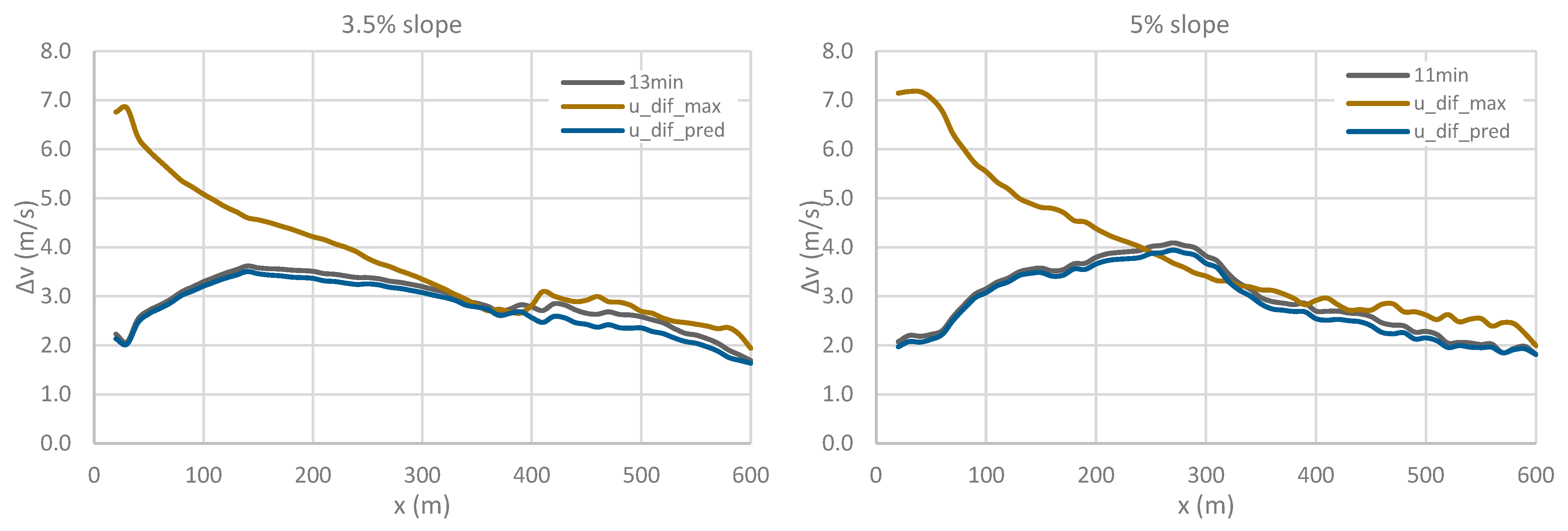
Figure 21 shows the lines corresponding to the predicted difference between the upper layer and lower layer velocities (u_dif_pred), which is obtained using Equations (27) and (32), and the maximum allowed velocity difference due to the temperature inside the tunnel (u_dif_max), which is given by Equation (33). The contamination by smoke starts at the intersection of these two lines, x_c. In the region to the right of x_c, the low value of the maximum allowed velocity difference due to the temperature inside the tunnel (u_dif_max) does not allow for the predicted upper layer and lower layers mass flow rates, and, therefore, the lower layer is contaminated by smoke.

The same figure shows the upper layer mass flow rate obtained in the CFD simulation (18 min MFR, 13 min MFR or 11 min MFR). In the region to the right of the peak, the lower layer is contaminated by smoke from the upper layer and the mass flow rate decreases.

Table 9. Longitudinal coordinate x_c (m) corresponding to the beginning of the lower layer smoke contamination.

	CFD Simulations	1D Model
1%	230	350
2%	300	300
3.5%	210	210
5%	270	130

compares the values of the peak of the upper layer mass flow rate (x_c) in the CFD simulations with the value of x_c obtained using the 1D model.

The results of the 1D model show that the value of x_c at the beginning of the contamination decreases when the slope increases. The predicted values obtained for 2% and 3.5% of slope coincide with the values obtained from the CFD simulation. However, the values of x_c obtained in the CFD simulations and in the 1D model for a slope of 1% are rather different because, as noted before, the contribution of the upper layer mass flow rate due to the mass transfer from the lower layer near the fire is more relevant for small slopes than for higher ones and this process is not considered in the present 1D model. In the case of a slope of 1%, when the initial upper layer mass flow rate obtained in the CFD simulations is used, the 1D model yields x_c = 290 m. This reveals that the initial value of the upper layer mass flow rate greatly influences the results and must be improved. The x_c value predicted for a slope of 5% is underpredicted when compared with the value obtained from the CFD simulations because the use of the average parameters obtained by the least squares fit of Equation (27) leads to the overprediction of the initial upper layer velocity v_u (x = 0), c and f factors (see Table 7 and Figure 18).

6. Conclusions

Systematic research on the processes that cause the lower layer smoke contamination in sloped tunnels has never been made. Therefore, the maximum length of a sloped tunnel that does not require the use of mechanical smoke control systems could not be estimated from the theory or data available in the literature. This problem is addressed in the present research, which investigates the propagation of smoke due to a fire in sloped tunnels. The CFD results allow the identification of the main processes of the contamination of the cold lower layer with smoke for a tunnel cross-section area of 60 m², a fire source of 13.5 MW and a slope between 1% and 5%. Three different regimes were identified, depending on the slope of the tunnel, namely, quasi-horizontal, transitional and quasi-forced ventilation regimes, for slopes lower than 1%, between 1% and 5%, and greater than 5%, respectively. The results show that the average mass flow rate in a sloped tunnel depends on the stack effect, which increases with the increase of the slope. The conclusions obtained for horizontal tunnels cannot be directly applied to sloped tunnels because, in the latter case, the magnitude of the upper layer average velocity is always higher than the magnitude of the lower layer average velocity. The average upper layer velocity near the fire may be determined from the momentum equation considering the buoyancy and the mass transfer between the two layers. When the tunnel cross-section cannot accommodate the mass flow rates of the upper and lower layers, the mixing between both layers starts, and the lower layer is contaminated. Therefore, the most relevant parameter to assess the beginning of the lower layer contamination is the peak of the upper layer mass flow rate. When this peak does not occur inside the tunnel, the lower layer will not be contaminated, and the users staying between the fire source and the upper portal will be inside the cold lower layer (for the dimensions of the tunnel of this research). In this case, it should not be required to install a mechanical smoke control system. A 1D analytical model to predict the location of the peak of the upper layer mass flow rate is presented, and it shows good agreement with the CFD results for slopes of 2% and 3.5% but needs to be improved for lower and higher slopes. It was also shown that the disturbance induced by a moderate external wind velocity (2.04 m/s) opposed to the upper layer velocity, at steady state, is significantly smaller in a tunnel with a slope of 2% than in a horizontal tunnel. Future work will focus on the analysis of the lower layer contamination with smoke considering other tunnel cross-sections and different fire source heat release rates.