Abstract
Weather forecasts are needed in fire management to support risk-based decision-making that considers both the probability of an outcome and its potential impact. These decisions are complicated by the large amount of uncertainty surrounding many aspects of the decision, such as weather forecasts. Wildland fires in Ontario, Canada can burn and actively spread for days, weeks, or even months, or be naturally limited or extinguished by rain. Conventional fire weather forecasts have typically been a single scenario for a period of one to five days. These forecasts have two limitations: they are not long enough to inform some fire management decisions, and they do not convey any uncertainty to inform risk-based decision-making. We present an overview of a method for the assembly and customization of forecasts that (1) combines short-, medium-, and long-term forecasts of different types, (2) calculates Fire Weather Indices and Fire Behaviour Predictions, including modelling seasonal weather station start-up and shutdown, (3) resolves differing spatial resolutions, and (4) communicates forecasts. It is used for burn probability modelling and other fire management applications.
1. Introduction
Wildland fire management decision-makers deal with a large amount of uncertainty, of which the future weather is a large contributor [1]. Weather forecasts support a variety of aspects of fire management, including predicting fire occurrence [2], behaviour (e.g., spread, intensity, and smoke) [3,4], and suppression effectiveness [5]. In the province of Ontario, Canada, the weather forecasts supporting wildland fire management decisions are generated by staff forecasters. These two-to-five-day forecasts inform near-term decisions, such as the deployment of firefighting resources and assessments of potential fire spread and impacts.
Assessing the risk of leaving a fire on the landscape requires considering the full duration of a fire to identify the possible effects. Fires may burn and spread for many days, weeks, or months if unsuppressed. In fire management, risk-based decision frameworks are used to account for the likelihood and impact of uncertain outcomes [1,6,7,8,9,10]. The use of multiple weather scenarios can incorporate uncertainty in such frameworks, e.g., [11].
The accuracy of weather forecasts is commonly recognized to decrease over the forecast period, and longer-term forecasts generally lack the detail needed to adequately model daily progressions in fire growth; specific daily weather components and fire weather indices may be missing. In addition, a forecast should not present a computational burden for burn probability models, e.g., [11] (i.e., stochastic fire growth simulation models used to predict fire growth and map the percentage of simulations that each cell burns). To our knowledge, there is no “off-the-shelf” solution for the long time horizon we need.
We present an approach developed by the Aviation Forest Fire and Emergency Services branch (AFFES) of the Ontario Ministry of Natural Resources and Forestry to assemble and customize different weather forecasts of different durations that were generated by different methods. We refer to this process by the acronym WeatherSHIELD (Weather, Short and Intermediate Ensemble and Long-term Dynamic scenarios). The forecast weather and corresponding Fire Weather Index System (FWI System) outputs of the Canadian Forest Fire Danger Rating System (CFFDRS) [4] are the inputs to burn probability and impact models [10]. The values are also displayed separately in a webtool. Prior to discussing our method in detail, we provide an overview of wildland fire management processes and decisions to motivate the need for our approach to assemble and customize weather forecasts.
Overview of Fire Management Processes and Decisions
Wildland fire management systems are complex, being driven by many highly uncertain and interacting factors [1]. In Ontario, conditions that drive fire occurrence and behaviour are highly variable spatially and temporally. Fire locations range from remote areas to urban interfaces. Daily fire occurrence ranges from low to very high, and fire behaviour ranges from low to extreme.
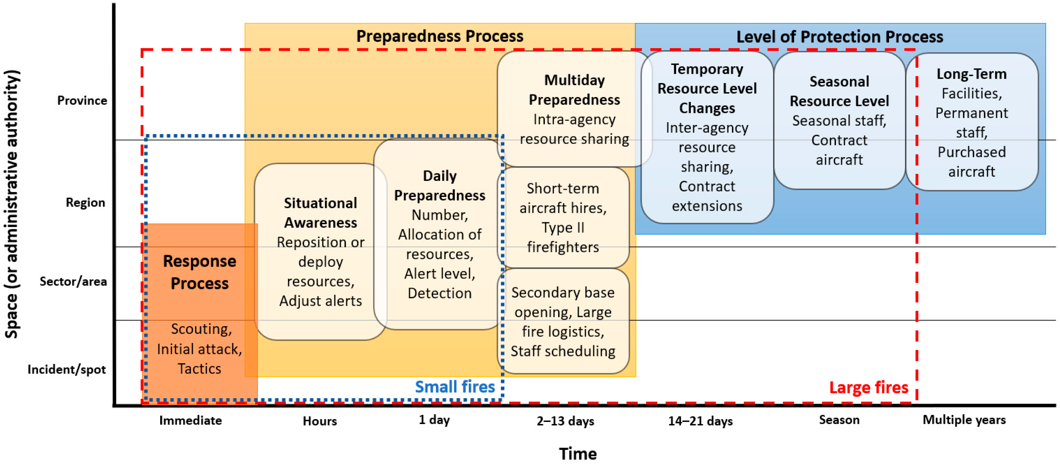
Fire management requires risk-based decision-making involving multiple spatial and temporal scales (Figure 1). Fire response decisions can be difficult, must often be made quickly, and have multiple impacts requiring difficult trade-offs. Decision-makers must consider multiple courses of action, all with uncertain outcomes. In addition, decisions and their outcomes have complex interactions and cascading effects [12,13]. To deal with this complexity and difficulty, wildland fire management agencies depend heavily on decision-makers who have a high level of experience and expertise.
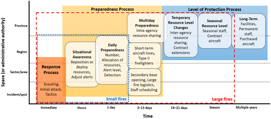
Figure 1.
Daily decision-making environment for wildland fire management in Ontario (adapted from [14,15,16]). The decision space for fire response takes place within the dashed boxes depending on the size, duration, impact, and complexity of the fire.
Fire response decisions (the left side of Figure 1) are generally the most urgent and are made by considering the impacts that will occur immediately or shortly after a fire occurs. Once a fire has been reported, rapid decisions about resource deployments and tactics are made considering the current and immediate forecast fire behaviour and associated impacts. In contrast, preparedness decisions (middle left of Figure 1) range from the short to intermediate term, e.g., 14 days, and deal more with ensuring adequate resource availability.
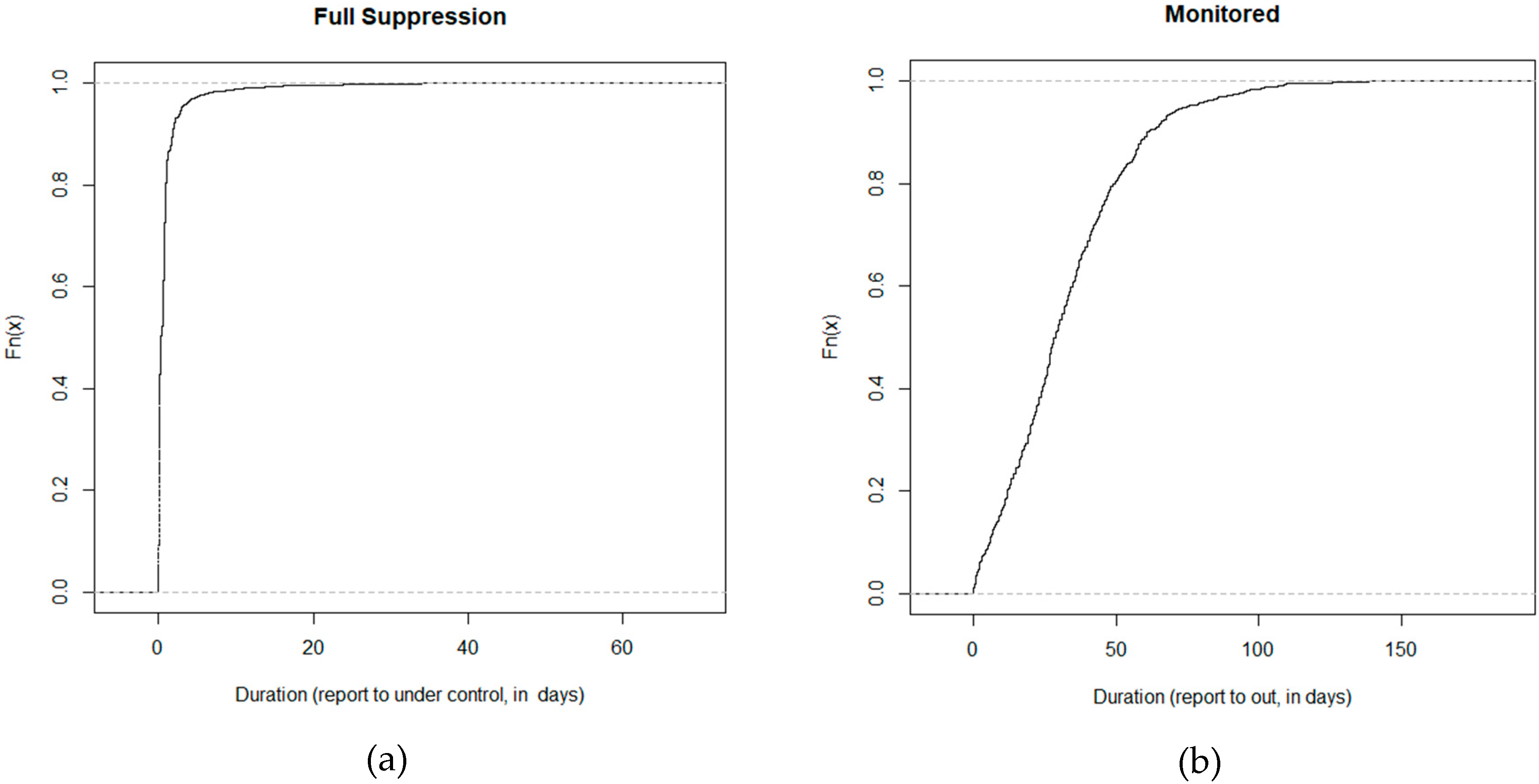
The time required to bring a fire under control is important because it affects resource commitment, costs, area burned, and impacts. The durations of suppressed and monitored fires provide context for the duration of forecasts needed. Figure 2 shows empirical cumulative distribution functions for the durations of full suppression (Figure 2a) and monitored (Figure 2b) fires in Ontario in 1990–2019. Most of the suppressed fires (~95%) are put out quickly or kept to a small size [17], so weather forecasts are not needed much further ahead than one to five days. The requirement is different, however, for monitored fires. In Ontario, fires that pose a low risk may be allowed to burn within predetermined boundaries until they are naturally extinguished [18,19]. For those decisions, a long-term forecast will help to assess the likelihood of having to return later and take suppression action. Some other jurisdictions also leave some low-risk fires on the landscape to facilitate natural ecological functioning or for other reasons. Even for the many jurisdictions that seek to suppress all fires, some fires may be partly or entirely unsuppressed for a time to prioritize limited suppression resources or because of extreme fire behaviour [12].
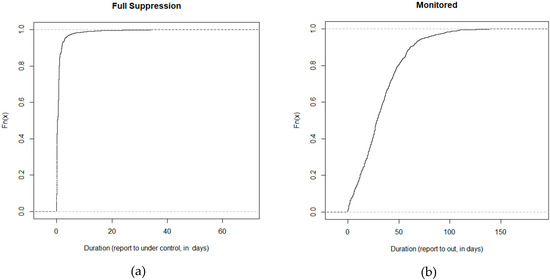
Figure 2.
Empirical cumulative distribution functions of fire duration (1990–2019) in Ontario, Canada, for: (a) Full suppression fires; (b) monitored fires. Duration is the time in days between reporting and being called “under control” for full suppression fires, or “out” for monitored fires. After data cleaning, there were 15,737 full suppression fires and 1457 monitored fires.
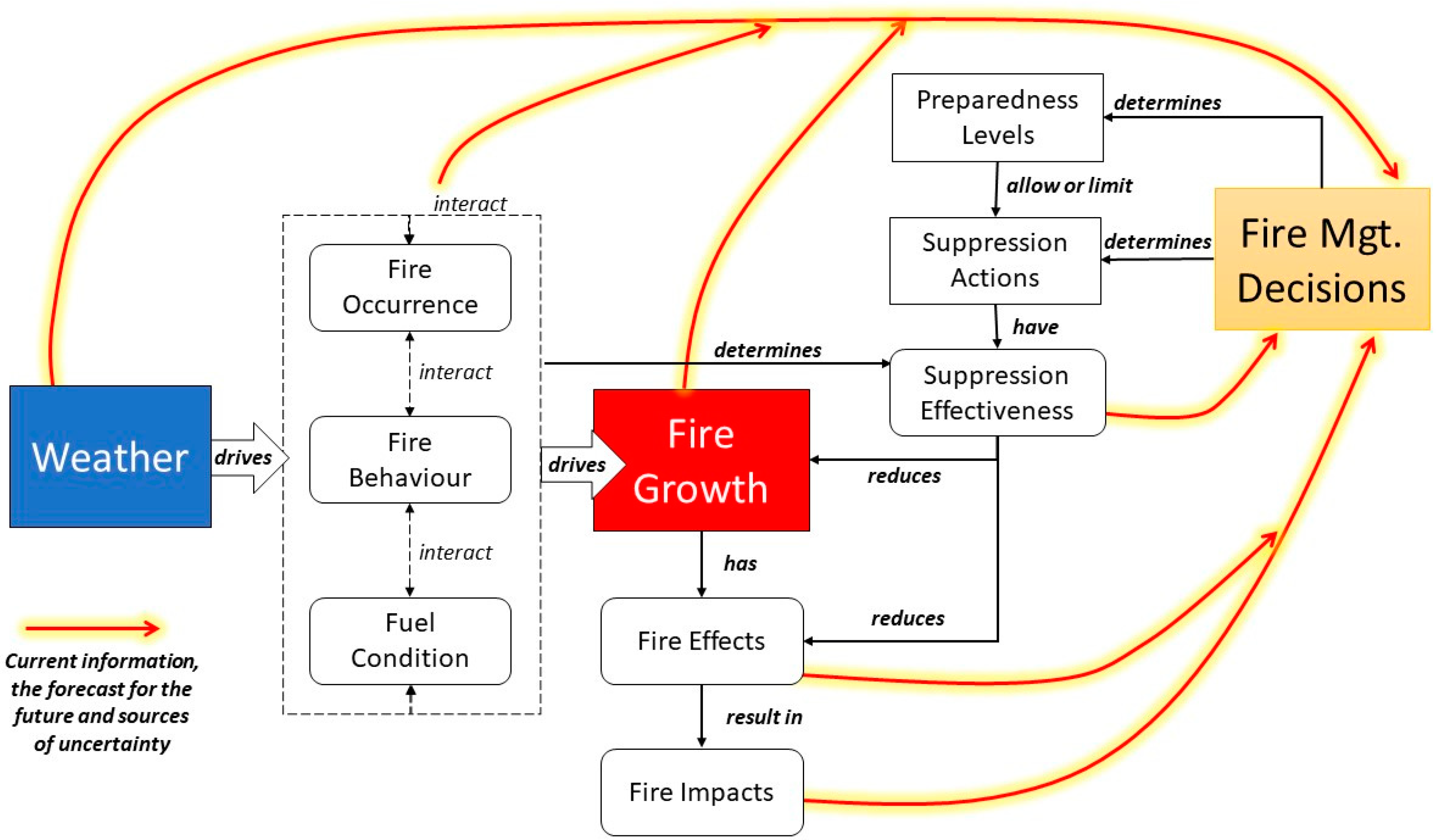
For all time horizons, the weather is a major driver of the fire environment and fire growth and therefore is a critical factor in decision-making. A simplified illustration of the links between weather, fire growth, effects, impacts, and decisions is given in Figure 3. The red and yellow arrows represent the information needed to inform decision-making now and in the future. Each element has its own aspects of uncertainty, but weather is at the root of the system. It drives fire occurrence, fire behaviour, and fuel conditions.
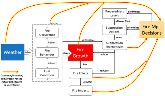
Figure 3.
Drivers and interactions among three core elements of the wildland fire system, namely weather, fire growth, and fire management decisions.
Given the weather’s influence on most fire management decisions over multiple spatial and temporal scales, there is a need to combine short-, medium-, and long-term weather forecasts into an integrated product. In what follows, we discuss a product that assembles component forecasts into a combined probabilistic forecast that provides input data for a fire growth model and also displays forecasts that decision-makers can view directly.
2. Methods
Our approach used the following steps:
- Step 1: Assembling three types and durations of forecasts;
- Step 2: Forecasting FWI System values and fire behaviour prediction values;
- Step 3: Reconciling spatial resolutions;
- Step 4: Communicating forecasts.
2.1. Step 1: Assembling Three Types and Durations of Forecasts
Short- and medium-term forecasts are a combination of ensemble weather forecasts and forecasts by AFFES weather forecasters. The numerical weather forecast ensemble we used is the North American Ensemble Forecast System (NAEFS) developed by the Meteorological Service of Canada, the U.S. National Weather Service, and the National Meteorological Service of Mexico [2,20]. NAEFS has 21 Global Ensemble Forecast System (GEFS) and 21 Global Ensemble Prediction System (GEPS) ensemble members (each with 20 perturbations and one control). AFFES weather forecasters create a single-scenario forecast by analysing multiple numerical weather models, weather observations, and other sources. The morning forecast is for two days, and the afternoon forecast update goes out to five days. In our approach, we extended the AFFES forecast to day 15 by appending the 42 NAEFS ensemble member values. In addition, the 42 NAEFS ensemble member values were used from day 1 to day 15, making a total of 84 weather scenarios over the first 15 days.
Longer-term weather forecast methods have not demonstrated the same success as short-term methods [21,22]. Methods vary in approach but generally rely on using historical weather or statistical techniques [11,23,24,25,26]. For day 16 onward, we used the historical daily weather components (temperature, relative humidity, precipitation, wind speed, and direction) from selected years in daily sequences [27]. This has important advantages over using synthetic weather data. First, it provides true weather system behaviour viz. complex autocorrelations among the weather components themselves and among weather over space and time (e.g., stationary high-pressure areas associated with extreme fire danger). Second, it retains local geographic variations. Given that teleconnections among SSTs and global weather patterns are widely recognized [28,29,30,31], we select “historical analogue years” based on the similarity of current and forecast sea surface temperature (SST) patterns (El Niño Southern Oscillation, Pacific Decadal Oscillation, and Atlantic Multidecadal Oscillation) to those in each of the historical years (Figure 4). This type of approach has been used informally by some experienced forecasters and in the scientific literature, e.g., [27].

Figure 4.
The steps in selecting historical analogue years for the long-term forecast.
We selected a subset of historical years for two reasons. First, simulating fires for all years from the historical data (73 years) presents an excessive computational burden for modelling burn probability, given our speed requirement and our available technology. Second, using years with similar SSTs is designed to select years that will provide either a better forecast (e.g., a drier spring may tend to occur with certain SST patterns) or at least an adequate forecast with fewer years. The number of historical analogue years to use is important. Using a small number of years shows trends (deviations from seasonal norms) most clearly but does not reflect the typical weather variability. In our quantitative model, however, we needed to represent variability, so we used more years. This is a trade-off: using more years may dilute the trend signals, while using fewer years may understate variability.
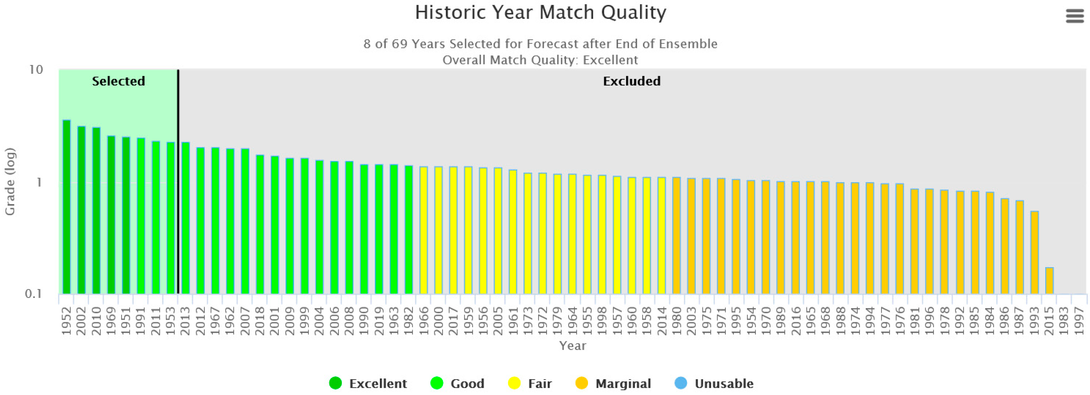
To select the historical analogue years, each year was given an SST pattern match score between 0–1. A “Score Sum”, which is a threshold value for the added match scores of the individual years, was preselected (currently we use 2.1). Years were selected starting from the highest-scoring year, until the sum of their match scores reached the Score Sum (Figure 5). The number and ranking of years selected varied, depending on the current and predicted SST values over the next six months. This made the long-term forecast dynamic rather than static, as would be the case if all historical years were used.
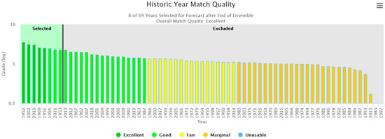
Figure 5.
Example of scored and selected historical analogue years, using a Score Sum of 2.1 (the y-axis is an intermediate variable related to the match score and is on a log scale). Years are classified by their match quality as being excellent, good, fair, poor, or unusable as selected historical analogue years.
Historical analogue years’ data were derived from the Reanalysis 1 [32], which has records from 1948 to the present. Reanalysis 1 was not an “actual” record in terms of measured fire weather station data, but a modelled estimate of past conditions based on a composite of multiple data sources. Furthermore, weather observations for fire weather required somewhat different weather station setups and observations than regular weather observations. Therefore, Reanalysis 1 outputs were calibrated to actual fire weather station observation records in Ontario to better approximate the weather variables that are used for FWI System inputs. Calibration was done by aligning the means and standard deviations or ranges based on data from proximate fire weather stations.
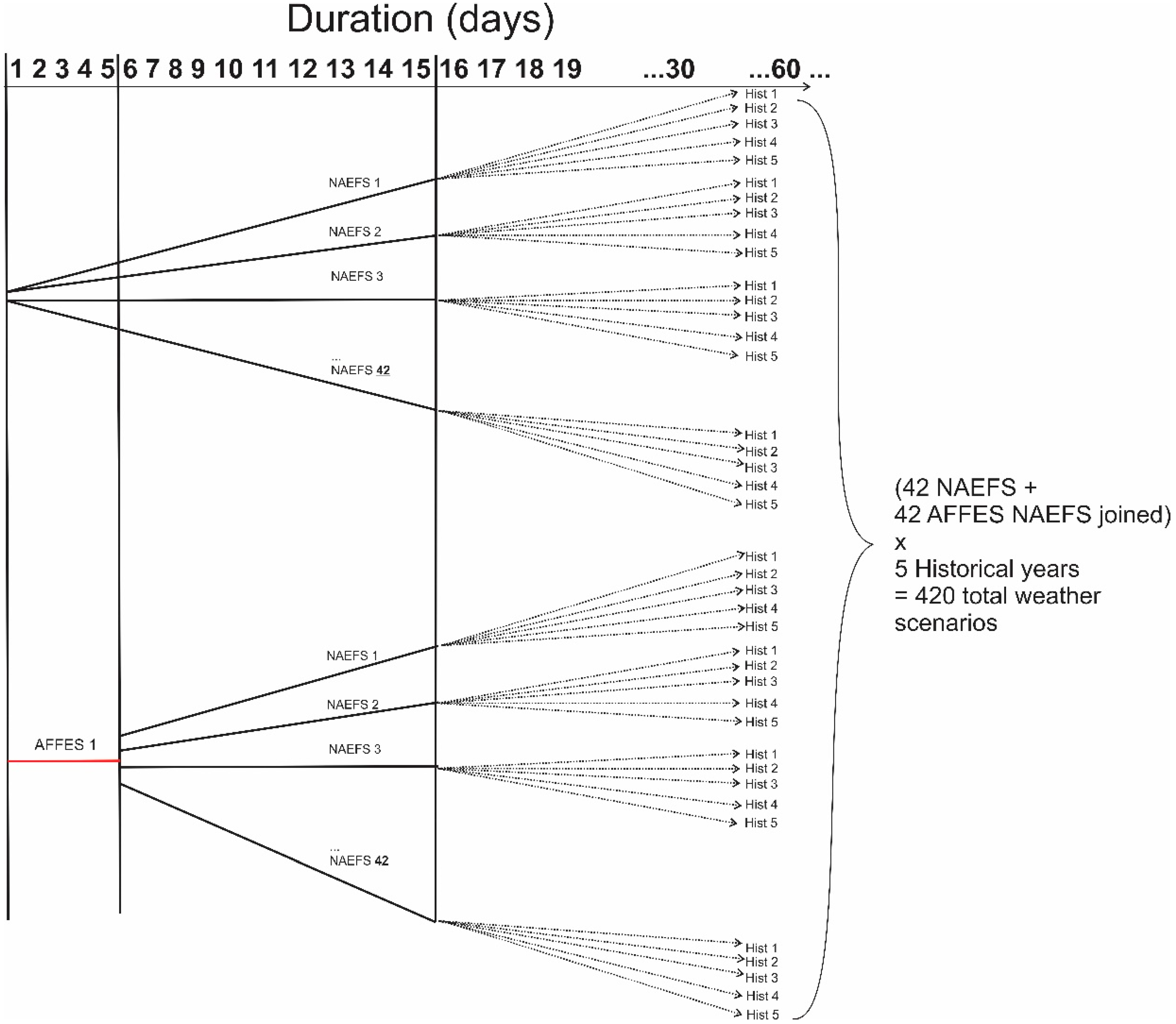
The historical weather data from each selected historical analogue year were appended to each endpoint of the forecast ensemble members (AFFES and AFFES + NAFES) after day 15. The total number of final weather scenarios depended on how many historical analogue years were used. The result was a variable number of weather scenarios that can number in the hundreds (Figure 6).

Figure 6.
An illustration of the number of distinct forecast scenarios increasing over the forecast horizon.
2.2. Step 2: Forecasting FWI System Values and Fire Behaviour Prediction Values
The predicted weather values were those required as inputs for the FWI System, namely daily 13:00 Local Daylight Time recordings of temperature, 24-h precipitation accumulation, relative humidity (RH), wind speed (10-min average) and direction [33,34]. Forecasting FWI System values is generally straightforward in the summer. The forecast weather was used to forecast FWI System values using the current values from the nearest weather station as the starting values. However, forecasting during the early spring or late fall requires estimates of when FWI System calculations will start and stop, respectively, when the ground is snow-free and snow-covered. To address this, we developed models based on observed relationships between weather conditions and when AFFES has historically started and stopped calculating FWI System values. The models also incorporate some physical relationships that would indicate snow-free or snow-covered situations. In Ontario, spring FWI System calculations generally begin following the first three-day period when the average forecasted 13:00 temperature equals or exceeds 11 °C. Fall FWI System calculations generally stop after the first three-day period when the average forecasted 13:00 temperature is below 2.5 °C and the Duff Moisture Code is less than 10, indicating a very wet forest floor organic layer, or following the first seven-day period where the average forecasted 13:00 temperature is less than 2.5 °C.
The weather inputs and corresponding FWI System values were then used to calculate fire behaviour, for which we used the CFFDRS’s Fire Behaviour Prediction System (FBP System) [35], which uses forest fuels, topography, and foliar moisture content to calculate quantitative estimates of potential head fire spread rate, fuel consumption, and fire intensity.
2.3. Step 3: Reconciling Spatial Resolutions
The component forecasts used in our forecast are provided for various gridded locations (Table 1). We used the forecast data from the nearest available points directly, i.e., without interpolation, e.g., [36,37]. We removed forecast source data points that were in or close to large bodies of water (e.g., the Great Lakes). This is to avoid having conditions over large water bodies being applied to land. The FWI System starting values were taken from the closest operating AFFES weather station, where one exists within 80 km, or according to the spring start-up rules described above in Step 2.

Table 1.
Spatial resolution of component forecasts and location of fire weather inputs.
2.4. Step 4: Communicating Forecasts
We had two human factors challenges in communicating the hundreds of forecast scenarios for the hundreds of forecast values (five weather components, six FWI System values, and 32 FBP System values for each forecast day). First, the voluminous information needs to be quickly interpretable, because decision-makers are often pressed for time. Second, the information needs to convey uncertainty, but seeing an explicit illustration of uncertainty is unfamiliar for most decision-makers. The way uncertainty is characterized can affect decision-making, e.g., [38,39].
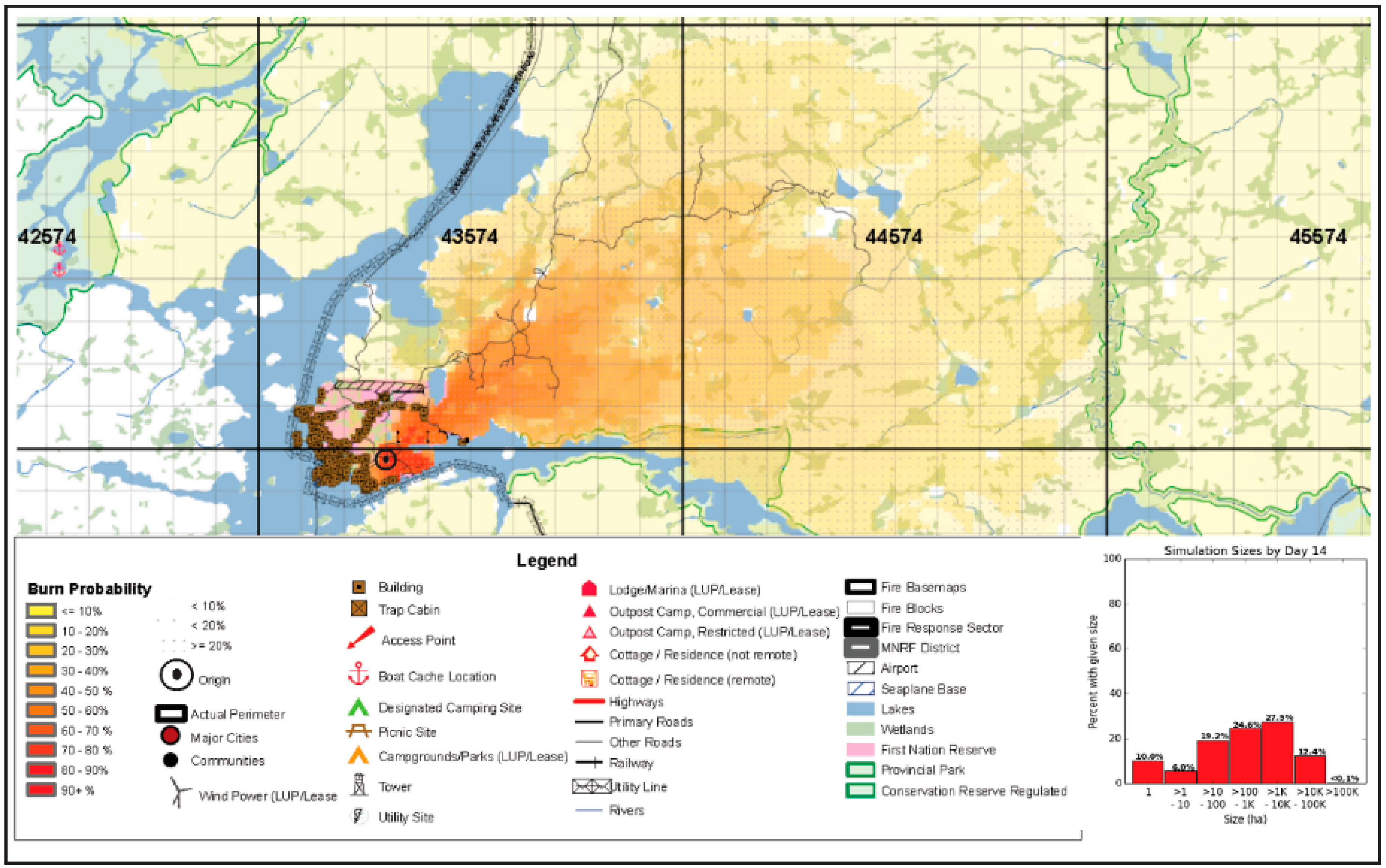
It is not the weather that is ultimately the most important metric of concern; rather, it is the fire activity that is influenced directly by the weather (Figure 3). A way to show this is by feeding the weather scenarios into a fire growth model, of which there are many. AFFES is developing a two-dimensional fire growth model, the Fire, Space-Time Alternating Recursive Rapid Growth burn probability model (FireSTARR) [40]. It has similar inputs and outputs to, e.g., Prometheus [41], including forecast weather, FWI System, and FBP System values; diurnal adjustment curves for wind and Fine Fuel Moisture Code (FFMC); and gridded fuel type and terrain data. The model outputs are fire perimeters at specified times ahead. The main practical difference from Prometheus is that some elements are stochastic. Running the stochastic fire growth model for each of the weather scenarios produces hundreds to thousands of different fire perimeters, which are combined into a burn probability map. The map’s cells are colour-coded by the 0% to 100% burn probability at a specified time ahead (Figure 7).
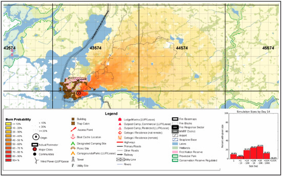
Figure 7.
An AFFES 14-day burn probability map from the FireSTARR model.
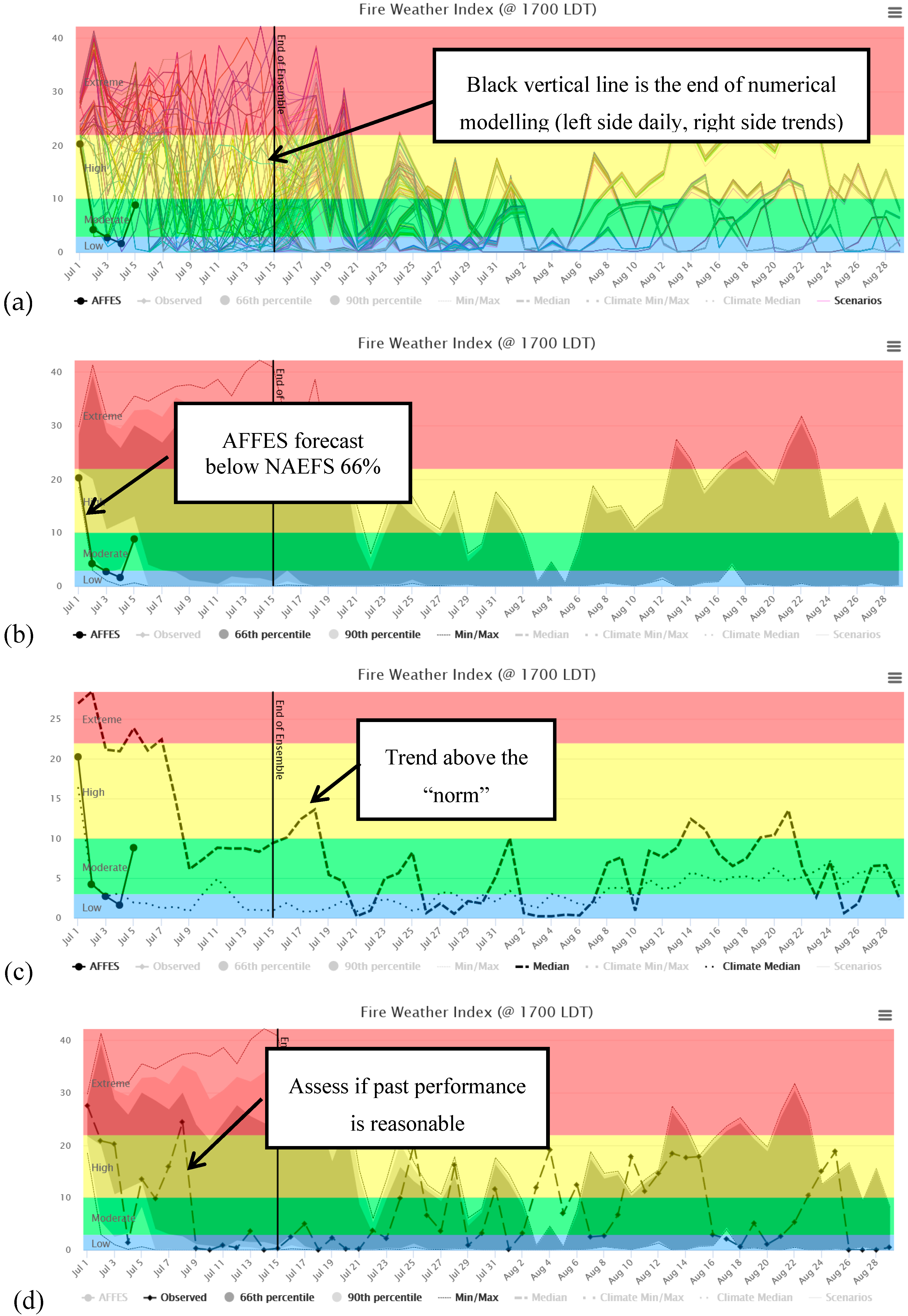
In addition to the burn probability maps, decision-makers wanted to be able to assess the individual weather, FWI System, and FBP System values that feed the burn probability model. They also wanted to use the forecasts to inform other decision-making (e.g., occurrence, control challenges, detection needs, and resource alerts). A webtool shows a chart for each weather value, FWI System value, and FBP System rate of spread for selected fuel types. Showing the individual scenarios is ineffective (Figure 8a), so the charts illustrate the probabilistic forecasts as medians, maxima, minima, and quantile bands: a middle 66% band and upper and lower 12% bands (Figure 8b). This shows the probability distribution of the forecast as prediction intervals that facilitate simple descriptions, e.g., 2/3 of the likelihood is between X and Y (the 66% band limits). Care must be taken to ensure that the users know that the median is not a single scenario (Figure 8c). The charts also show the maxima, minima, and median of all historical data, which highlights the deviation between the forecast and historical weather (Figure 8c). We colour the plot area backgrounds according to FWI System classification schemes (low to extreme) and FBP spread rates by class, e.g., low <5 m/min, extreme >20 m/min.
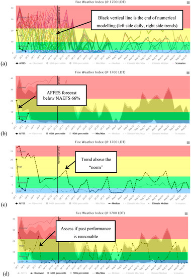
Figure 8.
Illustrations of a location’s 30-day forecast for FWI (Fire Weather Index) showing: (a) Individual scenarios; (b) prediction intervals; (c) medians for our forecast and for climatology as a forecast; (d) actual observations and the forecast for the period.
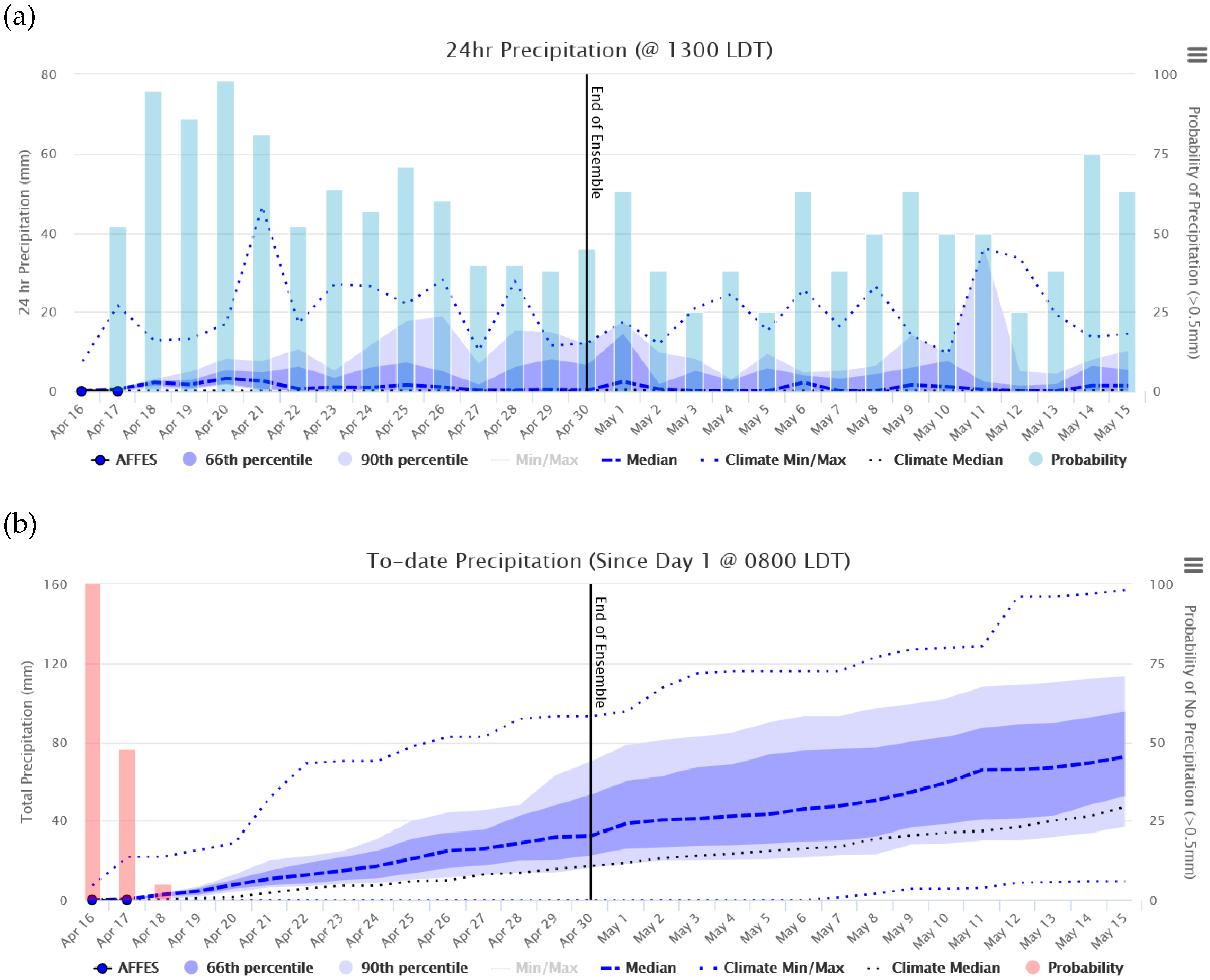
Precipitation is of special importance to decision-makers because it is the primary weather factor that that will provide relief to firefighting efforts. We plotted the probability of precipitation and to-date probability of no precipitation (Figure 9). The probability of precipitation is the percentage of forecast scenarios each day that have 24-h precipitation >0.5 mm (the threshold amount that affects the FWI System’s Fine Fuel Moisture Code) (Figure 9a). The to-date probability of no precipitation is the percentage of forecast scenarios that have had no precipitation >0.5 mm from 08:00 up to 13:00 on each day being forecasted (Figure 9b).

Figure 9.
(a) Daily precipitation and the daily probability of precipitation >0.5 mm; (b) to-date precipitation and the to-date probability of no precipitation >0.5 mm/day. The bars correspond to the right y-axis.
2.5. Verification
Regarding forecast verification, we address the informal and quantitative assessments of the forecast in various ways. For informal verification and to help users understand the accuracy of these forecasts, the webtool allows users to assess past forecasts by overlaying actual observations onto the forecast prediction intervals for the same dates (Figure 8d). This helps users learn the model’s degree of accuracy and gauge the level of confidence to place on the outputs. This is perhaps the most practical and useful operational verification in that it allows a user to determine if the performance has been “good enough” to warrant using it further.
Regarding quantitative verification, two of the component forecasts are verified elsewhere, so we did not further assess these components in isolation in the present work. Specifically, AFFES forecasters regularly evaluate their own forecasting performance and refine their products [42], and the NAEFS forecast has been well studied; there are numerous articles regarding how it performs, e.g., [43,44]. The use of selected historical analogue years based on SST pattern-matching, however, is expertise-based and experimental to AFFES; it has not been validated in the literature. We quantitatively assessed the performance of the combined forecast, because that is what is used operationally on its own and as an input to the burn probability model. This assessment was done using two widely used metrics: (1) the Brier Score [45] and (2) the relative operating characteristic area under the curve (ROC AUC) [46]. Forecasts are commonly evaluated by comparing their accuracy metrics to those of a reference forecast [47], often climatology, which is typically defined as weather over a 30-year period [48,49,50]. A forecast demonstrates “skill” when it beats a reference forecast [51]. The Brier Score provides one criterion for forecast skill, namely that the Brier Score calculated for the forecast is lower than the Brier Score calculated for climatology-as-a-forecast. The ROC AUC provides two criteria for forecasting skill, namely that the ROC AUC calculated for the forecast is simultaneously higher than the ROC AUC calculated for climatology-as-a-forecast and higher than a threshold value >0.5. Various threshold values have been used, e.g., [46]; we chose 0.6.
As for which of the many elements of a weather forecast to consider, it is of course very meaningful to verify temperature and precipitation forecasts [47], but we are most interested in the factors that drive active fire spread and intensity. As such, we focused on a verification analysis of FWI, which is a transformation of Byram’s fire line intensity [3]. FWI serves well as a single indicator of overall fire spread and behaviour potential, particularly from the fire suppression point of view. The FWI integrates the cumulative effects of weather over the preceding days and weeks through its dependence on the Buildup Index (BUI), which is a weighted average of the Duff Moisture Code (DMC) and Drought Code (DC). The latter two are indicators of the dryness of heavier and deeper fuels, which affects both fire intensity and the difficulty of extended suppression and mop-up work on larger fires. The FWI also integrates the effect on fire behaviour of fine fuel dryness and wind speed, which are driven by short-term weather conditions.
To use both the Brier Score and ROC AUC, the high-dimension forecast must necessarily be simplified to a single, discrete event that is being predicted [47], e.g., “FWI > 8”. A problem with using a constant threshold like FWI > 8 for the discrete event is that weather and typical fuel dryness changes significantly over the course of a season. We therefore used a variable threshold, e.g., “FWI > Xth percentile of historical FWI for that calendar day”. We chose to use the 80th percentile rather than the average or median because of the importance of the more extreme conditions. Choosing too high a percentile would be problematic, however, because the events would be very rare and inadequate for the Brier Score [45].
3. Results
This forecast method has been running in AFFES as (1) a stand-alone weather forecast display service since 2016 and (2) input to the prototype burn probability model since 2017. Over that time, the model status evolved from prototype testing to increasing operational use. The burn probability model replaced the previous, manual method in 78% of the extended Fire Assessment Reports completed in 2019. These reports are needed for the small percentage of fires that require extra assessment and documentation of the rationale for decision-making. This rapid uptake is a significant success. Decision support innovations can take years to be examined, evaluated, earn trust, and enter standard operating practise.
A quantitative analysis of forecast accuracy was performed on forecasts for the years with available forecast data (2017–2019) at one forecast location in Ontario (latitude 46.6658° N, longitude 80.625° W). The distance from the forecast location to the closest AFFES weather station, used for the starting fire weather indices, is ~22.6 km. The distances from the forecast location to the forecast source points were for AFFES 2.32 km, NAEFS’s GEFS 46.9 km, NAEFS’s GEPS 20.8 km and for Reanalysis 1 historical analogue year data 0 km. Within those years, the dates being forecasted were constrained to the range of June 1 to August 31 to eliminate problems with missing data due to variable spring start-up dates for the fire weather indices. For each of those dates, the forecasts from one to 90 days ahead were assembled for analysis.
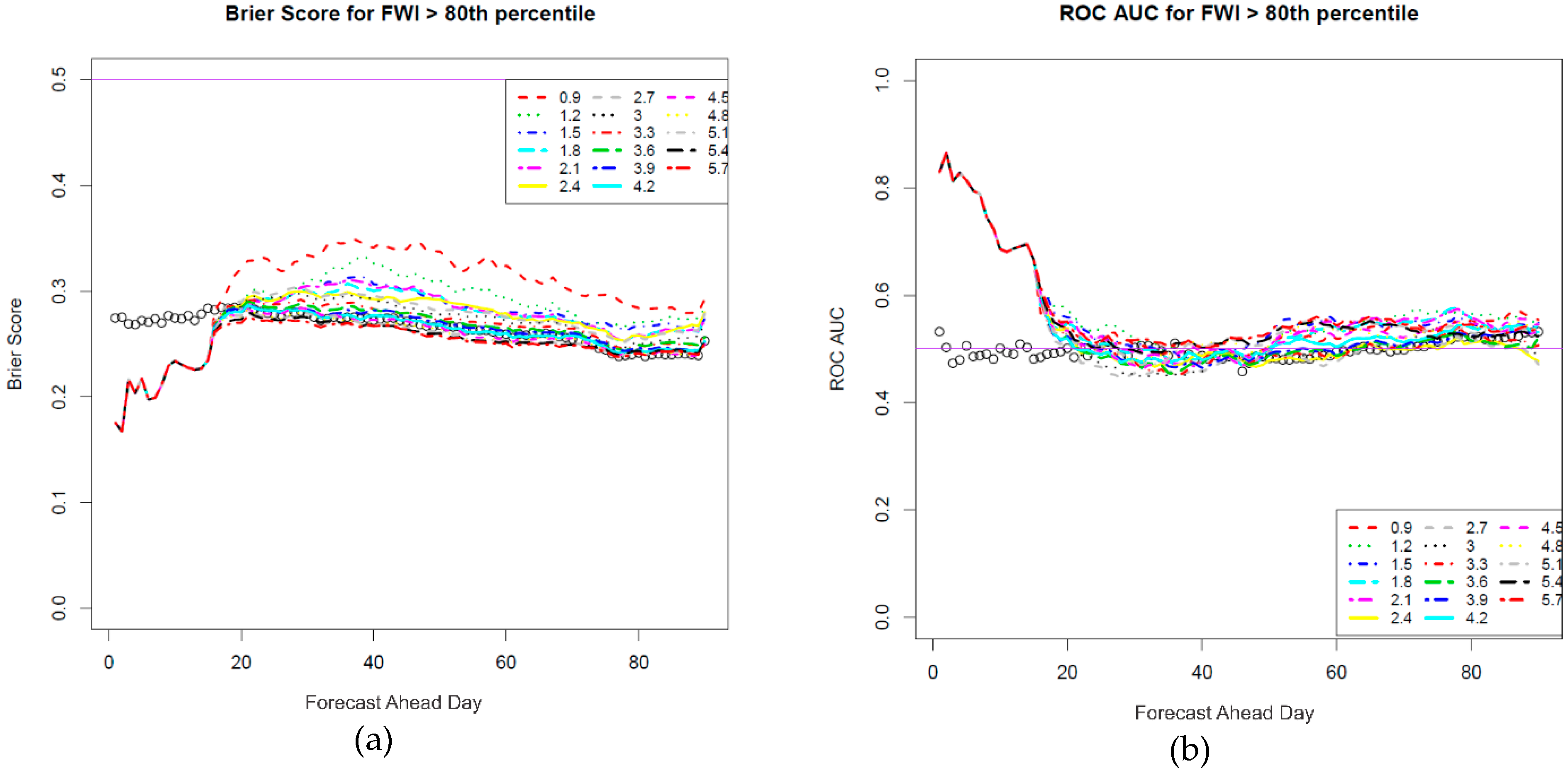
Regarding the quantitative assessment of the combined forecast, Figure 10 shows the Brier Score and ROC AUC for the event: “FWI > 80th percentile of climatology for the day being forecasted”. The plots show those measures for forecasts made from one to 90 days ahead, for both our assembled forecast and a climatology reference. As illustrated, the first 15 days exhibit the most skill in both the metrics. As expected, the AFFES forecasters and NAEFS component are much better compared to beyond day 15. Our selected historical analogue years range from a slightly lower to higher Brier Score than climatology, and generally a higher ROC AUC, although only just above the threshold of 0.6 at times depending on the number of historical years selected based on our “Score Sum” thresholds. Figure 10 suggests that we can improve the skill somewhat at the computational expense of including more years. Note that the median number of years selected at a Score Sum of 0.9 is around 1–2 and at a Score Sum of 5.7 it is close to 20.
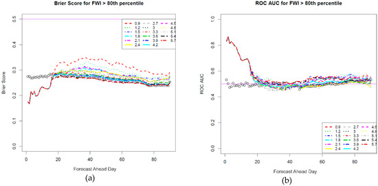
Figure 10.
(a) Brier Score; (b) relative operating characteristic (ROC) area under the curve (AUC) vs. the number of days ahead that the forecast was made (1–90). This is shown for various Score Sums (listed in the legend), which control the number of historical analogue years to append to day 15. The black circles are the measures for climatology. Our forecast’s (a) Brier Score should be below climatology’s to show “skill” when compared to climatology. Our forecast’s (b) ROC AUC should be above climatology’s to show “skill” and should exceed 0.6 (or at least be above 0.5 to suggest any skill compared to randomly guessing).
We also generated analogous results using all 10 of the weather and FWI System outputs. Results are summarized in Table 2, showing the days ahead where skill is demonstrated using a 2.1 Score Sum (a standard setting in operational use) and 5.1 (an example where more years will be selected) to determine the number of historical analogue years. The results of this example illustrate that the forecasts of the individual weather components are variable within the AFFES + NAEFS period, but interestingly, the FWI System components perform better for longer forecast horizons, depending on the Score Sum. This may be due to the fuel moisture indicators in the system, which integrate the effects of past weather over periods of days to weeks. The criteria for number of days showing skill in Table 2 is where the forecast has a lower Brier Score and higher ROC AUC (that is also over 0.6) than climatology up to the first day where climatology is the same or better. Note, this table does not show situations where the forecast and climatology metrics are the same.

Table 2.
Number of days for which our weather and fire weather forecasts are better than climatology as a forecast, based on Brier Score and ROC AUC > 0.6, for Score Sums 2.1 and 5.1. Italic numbers represent coverage to at least the 50th percentile of monitored fire duration (29 days).
We compared the duration frequencies of full suppression and monitored fires with the duration of forecast skill (Table 2). We see that almost all full suppression fires are covered by the AFFES + NAEFS forecast (99th percentile is 11 days). Around the 25th (16 days) to 50th percentile (29 days) of monitored fires are covered by adequate FWI forecasts with these different Score Sums. Note that monitored fires constitute only about 5% of fires in Ontario.
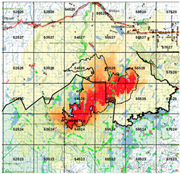
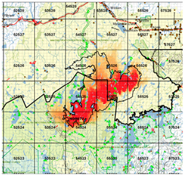
Regarding our goal of reducing the computational burden of fire growth modelling, Table 3 shows an example of the difference in using many historical years (71 years) and the selected years with a Score Sum of 2.1 for a single fire using FireSTARR. In this example, this saved close to 6 h of simulation time with arguably little practical difference in the areas of burn probability and median simulated fire sizes (see Table 3). Computations were done on a Windows 10 Professional x64 with an Intel(R) Xeon(R) CPU E5-2630 v3 @ 2.4 GHz 2.4 GHz (2 processors), 256 GB installed memory (RAM), a 64-bit operating system, and an installed solid-state drive.

Table 3.
Comparison of the computational burden and the burn probability maps when using the historical analogue years vs. all historical years as weather forecast scenarios. The black outline is the actual perimeter of the fire; the red-to-yellow gradient indicates burn probability. Note, fire simulations were initiated from a perimeter (10,396 ha).
4. Discussion
An assumption in using historical weather is that weather conditions in the future will resemble the weather of the past. This assumption will likely be challenged with the predicted effects of a changing climate on summer weather [52,53,54]. In any case, we recognize that specific historical weather sequences will not repeat in a period at a specific location [55]. With long-term forecasts, however, cumulative fire growth is more important than day-to-day accuracy (more below, with validation). A more difficult problem is the inevitable occurrence of rare events and record-breaking weather. Using historical data captures old but not new, rare events, which can be critical in fire management. Decision-makers need to account for this and other limitations of any forecast. Note that our long-term forecast can have record-breaking FWI System values, because they are recalculated from contemporary fuel moisture conditions and not taken directly from historically recorded FWI System values.
Note that the webtool currently excludes the AFFES forecast in the displayed prediction interval, i.e., the forecast median, 66% band, etc. The forecast weather scenarios that are input to the burn probability model do, however, incorporate the AFFES forecast as described above. Thus, users need to account for that subjectively when interpreting the input to the burn probability model. We separated the AFFES forecast from the displayed prediction interval because of the importance of the forecasters’ input and to highlight possible discussion points. Future versions may include the AFFES forecast.
We also note that our method does not indicate forecast confidence directly. It may perhaps be inferred indirectly by the degree to which the prediction interval is relatively tight. In general, however, forecast confidence is assessed by AFFES forecasters and relayed in briefings, especially for the two- to five-day AFFES forecasts. Incorporating confidence is an area of possible future work.
A limitation of our webtool that displays charts is that the charts apply to single locations, whereas decision-makers need situational awareness for large areas (up to areas larger than France). Plans are in place to map various probabilistic weather forecast outputs over specified time intervals, e.g., the probability of a spread event day occurring or the probability of some critical value of the FWI System being exceeded in the next three days, e.g., [56].
The use of historical analogue years has demonstrated usefulness for providing long-term weather forecast scenarios for burn probability modelling and other uses. We caution, however, that the long-term forecast has not demonstrated high skill. Simple improvements that can be made within our framework may be to increase the number of years or select them differently. A more complex issue is that the prediction interval is in a certain sense uniform, whereas we expect the uncertainty to widen over time. It is uniform because the number of historical analogue years remains the same over time. Simply widening the prediction intervals artificially using some type of statistical model is insufficient, because that would not produce corresponding forecast scenarios for the burn probability model. A possible alternative might be to add more historical analogue years at selected times ahead. This may be done easily by increasing the Score Sum every so many days. Or it may perhaps be done mechanistically by modelling future SST uncertainty, generating multiple SST scenarios and re-selecting historical analogue years every so many days. However, adding more years over the course of the forecast exponentially increases the number of scenarios. For example, if on day 40 we increased the number of historical analogue years from 5 to 8, the number of scenarios would increase not to 8 but to 20, because each of the initial five scenarios would split into four streams at day 40. E.g., Year 1 would continue with Year 1’s weather and also with Year 6, 7, and 8’s weather. We did not consider implementing any of this because of the computational burden. A widening prediction interval is an important problem for future research.
Regarding the constraint of computational burden, limiting the number of weather scenarios is not the only way to generate burn probability maps quickly. Using more powerful computing resources, such as extending parallel processing to multiple machines [57], is technically possible, but it would pose another kind of burden on our and many other agencies. Our weather forecast system and burn probability model can run on a single, ordinary, mid-range computer, although a solid-state drive helps.
There are, of course, many more verification methods than the two we used here (see, e.g., [47]). However, verification is not the primary focus of this paper. Further verification is planned, especially in concert with model refinements, evolution, or changes. An aspect of the validation metrics we used here is especially penalizing relative to what we expect to achieve using historical analogue years for our long-term forecasts. The Brier Score and ROC AUC calculate the metrics for the specific day ahead, e.g., day 37. We do not intend such long-term forecasts to have such fine resolution in time, i.e., they are not intended to be precise to the exact day, nor within a few days. We are working on indicators of forecast accuracy that consider realistic intentions about temporal resolution. There is an analogous problem with spatial resolution, which can be addressed, e.g., by entity-based verification methods [47].
The validation of a weather forecast technique over a large geographic extent and over a long period is a difficult task. We presented a simple diagnostic for one location. Brier Scores and other metrics are useful academically, but they are of little relevance to most end users since they do not represent how valuable the forecasts will be for their applications or in decision-making [58]. We can, however, use these metrics for calibration, e.g., for the Score Sum value, which affects the number of historical analogue years used in the long-term forecast. All predictions should have some form of objective validation; this is particularly important when systems are complex and environmental uncertainty is high. Engaging in regular assessment of predictions with standardized objective metrics will become increasingly important as we see new and complex methods brought to bear on forecasting in fire management.
Weather uncertainty is just one source that decision-makers must contend with, and each incident has unique challenges [1]. As the duration of a prediction gets longer, the uncertainly inherently gets larger as there are interactions with these other sources (e.g., natural stochasticity; limits in knowledge; unknown risk preferences) [1]. Adapting to conditions on a fire line is relatively simple compared to making larger strategic changes in preparedness. Even on a fire, as more is known and forecasts are updated, the situation is periodically reassessed and courses of action can be revised as often as necessary, until the fire is out [59]. The impact of being “wrong” with a forecast for tomorrow is higher than with a forecast for 30 days ahead because the forecast will be updated, and decisions revisited often over the interim.
Regardless of the uncertainty, people must make their decision. Thoughtful design must be put into these kinds of tools to avoid staff being overwhelmed by excessive, complex, or poorly structured information. Decision-makers will employ different strategies to cope with uncertainty [60] and we do not want to add to the burden by poorly designed models. Recent studies have explored the adoption of decision support tools and suggest opportunities to improve success, e.g., with training, involvement of staff and tailored design [61]. In all steps of our development, we involved the decision-makers—a key recommendation by Martell for successful implementation of decision support [62].
Fire management needs expert decision-makers, and many other factors will ultimately influence the decisions and decision-making process [63]. Short-, medium-, and long-term weather forecasts are an important element. We will use the best practical solutions available and will continue to seek improvements to all elements of our model. This process and its use are classed as experimental by AFFES and not considered the official agency forecast.
5. Conclusions
The development of this forecast process is the result of an operational fire management organization taking a novel approach to tackling a growing operational need: continuous long-range fire weather forecasts to support risk-based decision-making. The result is a process capable of creating one useable and continuous forecast from three distinct weather forecast methods: AFFES forecast staff (short-term), ensemble forecast (short- to medium-term), and an experimental scenario approach (long-term). This facilitates the automated application of weather experts’ knowledge for input to burn probability models and other decision support tools to help inform risk-based fire management decisions. Weather forecaster expertise is used in making the 2–5-day forecast and was crucial in the design of the long-term forecast method and design of how the three component forecasts were combined. Fundamentally, this process is a system for combining data to create information that supports an operational fire management need. The system was not intended to revolutionize fire weather forecasting, but rather to refine the use of existing forecast and historical data for long-term fire management decision-making. This process can be adapted to assemble different short-, medium-, and long-term forecasts as improvements are made to those methods.
Author Contributions
Conceptualization, D.B., J.E., D.J., C.B.M., A.S., J.S., and M.W.; methodology, D.B., J.E., D.L., C.B.M., D.G.M., A.S., J.S., and M.W.; software, J.E. and A.S.; validation, D.B., C.B.M., A.S., and D.G.W.; formal analysis, D.B., C.B.M., A.S., and D.G.W. and J.E.; data curation, J.E., A.S., and J.S.; writing—original draft preparation, D.B., D.J., C.B.M., D.G.W., and M.W.; writing—review and editing, D.B., J.E., D.J., D.L., C.B.M., D.G.M., A.S., J.S., D.G.W., and M.W.; visualization, D.B., J.E., D.L., C.B.M., D.M., A.S., J.S., D.G.W., and M.W.; project administration, D.B., C.B.M., and D.M. All authors have read and agreed to the published version of the manuscript.
Funding
We acknowledge the support of the Natural Sciences and Engineering Research Council of Canada (NSERC) to Douglas Woolford (funding reference number: RGPIN-2015–04221).
Acknowledgments
Thank you to the Ontario Ministry of Natural Resources and Forestry for support and AFFES staff, including Randal Kuyvenhoven, Benito Russo, and Melanie Wheatley for helpful contributions. We especially thank the management team for support, including Bill Cole, Dan Lasante, John R. MacDonald, Stephanie Maragna, Rob McAlpine, and Al Tithecott. Thank you, Mike Flannigan (University of Alberta), David L. Martell (University of Toronto), and Joshua M. Johnston (Canadian Forest Service), for valuable contributions and advice. We thank the two anonymous referees and the academic editor for their reviews that helped us significantly improve the manuscript.
Conflicts of Interest
The authors declare no conflict of interest.
References
- Thompson, M.P.; Calkin, D.E. Uncertainty and risk in wildland fire management: A review. J. Environ. Manag. 2011, 92, 1895–1909. [Google Scholar] [CrossRef] [PubMed]
- Wotton, B.M.; Martell, D.L. A lightning fire occurrence model for Ontario. Can. J. For. Res. 2005, 35, 1389–1401. [Google Scholar] [CrossRef]
- Van Wagner, C.E. Development and Structure of the Canadian Forest Fire Weather Index System; Forestry Technical Report; Canada Communication Group Publication: Ottawa, ON, Canada, 1987; ISBN 9780662151982. [Google Scholar]
- Stocks, B.J.; Lynham, T.J.; Lawson, B.D.; Alexander, M.E.; Wagner, C.E.V.; McAlpine, R.S.; Dubé, D.E. Canadian Forest Fire Danger Rating System: An Overview. For. Chron. 1989, 65, 258–265. [Google Scholar] [CrossRef]
- Hirsch, K.; Martell, D. A Review of Initial Attack Fire Crew Productivity and Effectiveness. Int. J. Wildland Fire 1996, 6, 199. [Google Scholar] [CrossRef]
- Johnston, L.M.; Wang, X.; Erni, S.; Taylor, S.W.; McFayden, C.B.; Oliver, J.A.; Stockdale, C.; Christianson, A.; Boulanger, Y.; Gauthier, S.; et al. Wildland fire risk research in Canada. Environ. Rev. 2020, 1–23. [Google Scholar] [CrossRef]
- Calkin, D.E.; Thompson, M.P.; Finney, M.A.; Hyde, K.D. A real-time risk assessment tool supporting wildland fire decision-making. J. For. 2011, 109, 274–280. [Google Scholar]
- Scott, J.H.; Thompson, M.P.; Calkin, D.E. A Wildland Fire Risk Assessment Framework for Land and Resource Management; General Technical Report RMRSGTR-315; USDA Forest Service, Rocky Mountain Research Station: Ogden, UT, USA, 2013.
- Finney, M.A. The challenge of quantitative risk analysis for wildland fire. For. Ecol. Manag. 2005, 211, 97–108. [Google Scholar] [CrossRef]
- McFayden, C.B.; Boychuk, D.; Woolford, D.G.; Wheatley, M.J.; Johnston, L. Impacts of wildland fire effects on resources and assets through expert elicitation to support fire response decisions. Int. J. Wildland Fire 2019, 28, 885. [Google Scholar] [CrossRef]
- Finney, M.A.; Grenfell, I.C.; McHugh, C.W.; Seli, R.C.; Trethewey, D.; Stratton, R.D.; Brittain, S. A Method for Ensemble Wildland Fire Simulation. Environ. Model Assess 2011, 16, 153–167. [Google Scholar] [CrossRef]
- Tymstra, C.; Stocks, B.J.; Cai, X.; Flannigan, M.D. Wildfire management in Canada: Review, challenges and opportunities. Prog. Disaster Sci. 2020, 5, 100045. [Google Scholar] [CrossRef]
- Natural Resources Canada, Fire Management. Available online: https://www.nrcan.gc.ca/our-natural-resources/forests-forestry/wildland-fires-insects-disturban/forest-fires/fire-management/13157 (accessed on 17 May 2020).
- Simard, S. Fire Severity, Changing Scales, and How Things Hang Together. Int. J. Wildland Fire 1991, 1, 23. [Google Scholar] [CrossRef]
- Taylor, S.W. Review and discussion of fire management resource demand and capacity planning models. 2011; unpublished. [Google Scholar]
- McFayden, C.; Boychuk, D. Fire Management Decisions. In Workshop on Evolving Marked Point Processes with Application to Wildland Fire Regime Modeling; FIELDS Institute: Toronto, ON, Canada, 2015. [Google Scholar]
- Morin, A.A.; Albert-Green, A.; Woolford, D.G.; Martell, D.L. The use of survival analysis methods to model the control time of forest fires in Ontario, Canada. Int. J. Wildland Fire 2015, 24, 964. [Google Scholar] [CrossRef]
- Boychuk, D.; McFayden, C. Appropriate response—Ontario’s strategic approach to wildland fire. In Canadian Wildland Fire and Smoke Newsletter; Canada Wildfire: Edmonton, AB, Canada, 2017; Available online: https://docs.wixstatic.com/ugd/90df79_bfcc500b532a4e38abaa78e1ecfdd26b.pdf (accessed on 17 May 2020).
- Ontario Ministry of Natural Resources and Forestry. Wildland Fire Management Strategy; Queen’s Printer for Ontario: Toronto, ON, Canada, 2014.
- Toth, Z.; Desmarais, J.G.; Brunet, G.; Zhu, Y.; Verret, R.; Wobus, R.; Hogue, R.; Cui, B. The North American ensemble forecast system (NAEFS). Geophys. Res. Abstr. 2005, 7, 02501. [Google Scholar]
- Epstein, E. Long-Range Weather Prediction: Limits of Predictability and Beyond. Weather Forecast. 1988, 3, 69–75. [Google Scholar] [CrossRef]
- Zhang, F.; Sun, Y.Q.; Magnusson, L.; Buizza, R.; Lin, S.-J.; Chen, J.-H.; Emanuel, K. What Is the Predictability Limit of Midlatitude Weather? J. Atmos. Sci. 2019, 76, 1077–1091. [Google Scholar] [CrossRef]
- McAlpine, R.S. Seasonal Trends in the Drought Code Component of the Canadian Forest Fire Weather Index System; Report. no. PI-X-97E/F; Forestry Canada, Petawawa National Forestry Institute: Chalk River, ON, Canada, 1990. [Google Scholar]
- Anderson, K.R.; Englefield, P.; Carr, R. Predicting fire-weather severity using seasonal forecasts. In Proceedings of the 7th Symposium on Fire and Forest Meteorology, Bar Harbor, ME, USA, 23–25 October 2007; American Meteorological Society: Boston, MA, USA, 2007. [Google Scholar]
- Anderson, K. A climatologically based long-range fire growth model. Int. J. Wildland Fire 2010, 19, 879. [Google Scholar] [CrossRef]
- Pence, M.; Zimmerman, T. The Wildland Fire Decision Support System: Integrating science, technology, and fire management. Fire Manag. Today 2011, 71, 18–22. [Google Scholar]
- Toth, Z. Long-range weather forecasting using an analog approach. J. Clim. 1989, 2, 594–607. [Google Scholar] [CrossRef]
- Bonsal, B.; Lawford, R. Teleconnections between El Niño and La Niña events and summer extended dry spells on the Canadian Prairies. Int. J. Climatol. 1999, 19, 1445–1458. [Google Scholar] [CrossRef]
- NOAA National Centers for Environmental Information, El Niño/Southern Oscillation (ENSO) Technical Discussion. Available online: www.ncdc.noaa.gov/teleconnections/enso/enso-tech.php (accessed on 17 May 2020).
- Skinner, W.R.; Stocks, B.J.; Martell, D.L.; Bonsal, B.; Shabbar, A. The Association Between Circulation Anomalies in the Mid-Troposphere and Area Burned by Wildland Fire in Canada. Theor. Appl. Climatol. 1999, 63, 89–105. [Google Scholar] [CrossRef]
- Wang, Y.; Flannigan, M.; Anderson, K. Correlations between forest fires in British Columbia, Canada, and sea surface temperature of the Pacific Ocean. Ecol. Model. 2010, 221, 122–129. [Google Scholar] [CrossRef]
- Kalnay, E.; Kanamitsu, M.; Kistler, R.; Collins, W.; Deaven, D.; Gandin, L.; Iredell, M.; Saha, S.; White, G.; Woollen, J.; et al. The NCEP/NCAR 40-Year Reanalysis Project. Bull. Am. Meteorol. Soc. 1996, 77, 437–471. [Google Scholar] [CrossRef]
- Turner, J.; Lawson, B. Weather in the Canadian forest fire danger rating system. In A User Guide to National Standards and Practices; Report. no. BC-X-177; Fisheries and Environment Canada, Canadian Forest Service, Pacific Forest Research Centre: Victoria, BC, Canada, 1978. [Google Scholar]
- Lawson, B.D.; Armitage, O.B.; Northern Forestry Centre (Canada). Weather Guide for the Canadian Forest Fire Danger Rating System; Canadian Forest Service, Northern Forestry Centre: Edmonton, AB, Canada, 2008; ISBN 9781100115658.
- Forestry Canada Fire Danger Group. Development and Structure of the Canadian Forest Fire Behavior Prediction System; Information report ST-X-3; Forestry Canada, Science and Sustainable Development Directorate: Ottawa, ON, Canada, 1992; ISBN 9780662198123.
- Flannigan, M.D.; Wotton, B.M. A study of interpolation methods for forest fire danger rating in Canada. Can. J. For. Res. 1989, 19, 1059–1066. [Google Scholar] [CrossRef]
- Jain, P.; Flannigan, M.D. Comparison of methods for spatial interpolation of fire weather in Alberta, Canada. Can. J. For. Res. 2017, 47, 1646–1658. [Google Scholar] [CrossRef]
- Tversky, A.; Kahneman, D. Judgment under uncertainty: Heuristics and biases. In Utility, Probability, and Human Decision Making; Springer: Dordrecht, The Netherlands, 1975; pp. 141–162. [Google Scholar]
- Maguire, L.A.; Albright, E.A. Can behavioral decision theory explain risk-averse fire management decisions? For. Ecol. Manag. 2005, 211, 47–58. [Google Scholar] [CrossRef]
- Boychuk, D.; Evens, J.; Leonard, D.; McFayden, C.; McLarty, D.; Wotton, M. FireSTARR: Automated Burn Probability Maps within Minutes of Every Fire Report in Ontario, Canada. Presented at Wildland Fire Canada, Ottawa, ON, Canada, 18–21 November 2019. [Google Scholar]
- Tymstra, C.; Bryce, R.W.; Wotton, B.M.; Taylor, S.W.; Armitage, O.B. Development and Structure of Prometheus: The Canadian Wildland Fire Growth Simulation Model; Northern Forestry Centre: Edmonton, AB, Canada, 2010; p. 102.
- Shields, J. The Future of Fire Weather Forecasting: Human vs. Computer Forecasting; Wildland Fire Canada: Kelowna, BC, Canada, 2016; Available online: http://www.wildlandfire2016.ca/wp-content/uploads/2017/02/Future-of-Fire-Weather-Forecasting-Shields.pdf (accessed on 17 May 2020).
- Candille, G. The Multiensemble Approach: The NAEFS Example. Mon. Weather Rev. 2009, 137, 1655–1665. [Google Scholar] [CrossRef]
- Gneiting, T.; Balabdaoui, F.; Raftery, A.E. Probabilistic forecasts, calibration and sharpness. J. R. Stat. Soc. B 2007, 69, 243–268. [Google Scholar] [CrossRef]
- Brier, G.W. Verification of forecasts expressed in terms of probability. Mon. Weather Rev. 1950, 78, 1–3. [Google Scholar] [CrossRef]
- Hosmer, D.W.; Lemeshow, S. Applied Logistic Regression; John Wiley & Sons, Inc.: Hoboken, NJ, USA, 2000; ISBN 9780471722144. [Google Scholar]
- Wilks, D.S. Statistical Methods in the Atmospheric Sciences, 3rd ed.; International Geophysics Series; Elsevier/Academic Press: Amsterdam, The Netherlands; Boston, MA, USA, 2011; ISBN 9780123850225. [Google Scholar]
- Government of Canada. Canadian Climate Normals. Available online: https://climate.weather.gc.ca/climate_normals (accessed on 17 May 2020).
- NOAA. Climate Normals. Available online: https://www.ncdc.noaa.gov/data-access/land-based-station-data/land-based-datasets/climate-normals (accessed on 17 May 2020).
- Government of Canada. Technical Documentation Climate Normals. Available online: https://www.canada.ca/en/environment-climate-change/services/climate-change/canadian-centre-climate-services/display-download/technical-documentation-climate-normals.html#toc1 (accessed on 17 May 2020).
- World Climate Research Program. WWRP/WGNE Joint Working Group on Forecast Verification Research. Available online: https://www.cawcr.gov.au/projects/verification (accessed on 17 May 2020).
- Flannigan, M.D.; Logan, K.A.; Amiro, B.D.; Skinner, W.R.; Stocks, B.J. Future Area Burned in Canada. Clim. Chang. 2005, 72, 1–16. [Google Scholar] [CrossRef]
- Wotton, B.; Martell, D.; Logan, K. Climate change and people-caused forest fire occurrence in Ontario. Clim. Chang. 2003, 60, 275–295. [Google Scholar] [CrossRef]
- Wotton, M.; Logan, K.; McAlpine, R.S. Climate Change and the Future Fire Environment in Ontario: Fire Occurrence and Fire Management Impacts; Applied Research and Development Branch, Ontario Ministry of Natural Resources: Sault Ste. Marie, ON, Canada, 2010; ISBN 9780779455621. [Google Scholar]
- Jianping, H.; Yuhong, Y.; Shaowu, W.; Jifen, C. An analogue-dynamical long-range numerical weather prediction system incorporating historical evolution. Q. J. R. Meteorol. Soc. 1993, 119, 547–565. [Google Scholar] [CrossRef]
- Government of Canada. NAEFS Probability Maps of Weather Events over Time Intervals. Available online: https://weather.gc.ca/ensemble/naefs/produits_e.html (accessed on 17 May 2020).
- Bogdos, N.; Manolakos, E.S. A tool for simulation and geo-animation of wildfires with fuel editing and hotspot monitoring capabilities. Environ. Model. Softw. 2013, 46, 182–195. [Google Scholar] [CrossRef]
- Mylne, K.R. Decision-making from probability forecasts based on forecast value. Meteorol. Appl. 2002, 9, 307–315. [Google Scholar] [CrossRef]
- Taber, M.A.; Elenz, L.M.; Langowski, P.G. Decision Making for Wildfires: A Guide for Applying a Risk Management Process at the Incident Level; U.S. Department of Agriculture, Forest Service, Rocky Mountain Research Station: Fort Collins, CO, USA, 2013; p. 59, RMRS-GTR-298WWW.
- Lipshitz, R.; Strauss, O. Coping with Uncertainty: A Naturalistic Decision-Making Analysis. Organ. Behav. Hum. Decis. Process. 1997, 69, 149–163. [Google Scholar] [CrossRef]
- Noble, P.; Paveglio, T.B. Exploring Adoption of the Wildland Fire Decision Support System: End User Perspectives. J. For. 2020, 118, 154–171. [Google Scholar] [CrossRef]
- Martell, D. The development and implementation of forest and wildland fire management decision support systems: Reflections on past practices and emerging needs and challenges. Math. Comput. For. Nat. Resour. Sci. 2011, 3, 18. [Google Scholar]
- Hutton, R.J.; Klein, G. Expert decision making. Syst. Eng. 1999, 2, 32–45. [Google Scholar] [CrossRef]
© 2020 by the authors. Licensee MDPI, Basel, Switzerland. This article is an open access article distributed under the terms and conditions of the Creative Commons Attribution (CC BY) license (http://creativecommons.org/licenses/by/4.0/).

