Ground Penetrating Radar Investigation of Late Pleistocene Shorelines of Pluvial Lake Clover, Elko County, Nevada, USA

Abstract

Beach ridges constructed by pluvial Lake Clover in Elko County, Nevada during the Late Pleistocene were investigated with ground-penetrating radar (GPR). The primary objective was to document the internal architecture of these shorelines and to evaluate whether they were constructed during lake rise or fall. GPR data were collected with a ground-coupled 400-Mhz antenna and SIR-3000 controller. To constrain the morphology of the ridges, detailed topographic surveys were collected with a Topcon GTS-235W total station referenced to a second class 0 vertical survey point. GPR transects crossed the beach ridge built by Lake Clover at its highstand of 1725 m, along with seven other ridges down to the lowest beach at 1712 m. An average dielectric permittivity of 5.0, typical for dry sand and gravel, was calculated from GPR surveys in the vicinity of hand-excavations that encountered prominent stratigraphic discontinuities at known depths. Assuming this value, consistent radar signals were returned to a depth of ~3 m. Beach ridges are resolvable as ~90 to 150-cm thick stratified packages of gravelly sand overlying a prominent lakeward-dipping reflector, interpreted as the pre-lake land surface. Many ridges contain a package of sediment resembling a buried berm at their core, typically offset in a landward direction from the geomorphic crest of the beach ridge. Sequences of lakeward-dipping reflectors are resolvable beneath the beach face of all ridges. No evidence was observed to indicate that beach ridges were submerged by higher water levels after their formation. Instead, the GPR data are consistent with a model of sequential ridge formation during a monotonic lake regression.

1. Introduction

A large area of southwestern North America, known as the Great Basin, is internally drained, offering no route to the ocean for surface water [1]. Owing to its arid climate in the rain shadow of the Sierra Nevada, fresh surface water is rare in this region today [2]. However, during wetter “pluvial” climates of the Pleistocene, numerous large lakes occupied local low-points within this overall endorheic topography [3,4]. Although the former presence of extensive surface water is challenging to visualize in such an arid landscape, the pluvial lakes are represented by indisputable geomorphic evidence in the form of beach berms, spits, bars, and wave-cut terraces, many of which have been recognized for over a century [5,6,7]. The pluvial lakes are, therefore, the most iconic evidence for the profound hydroclimate variability that accompanied glacial-interglacial cycles in this part of North America.

Despite their significance as indicators of paleoclimate conditions, pluvial lakes are challenging topics of study. Their sediments are typically devoid of organic materials suitable for radiocarbon dating, and where present, shells and other remains of aquatic organisms may be vulnerable to hard-water effects of uncertain magnitude [8]. Application of other geochronometers such as U-series dating, luminescence, amino acid racemization, and cosmogenic surface-exposure techniques, can yield results that are difficult to interpret [9,10]. Although aerial and satellite imagery combined with geospatial information systems can facilitate the identification and mapping of pluvial lake shorelines, many of these landforms are located in remote areas making field investigations challenging. In addition, natural exposures in pluvial lake beaches and berms are rare, meaning that stratigraphic investigations are typically limited to snapshot views provided by hand excavations. Even in situations where heavy equipment is used to create larger windows into the subsurface, either for sand and gravel mining or specifically for scientific investigation e.g. [11], the scale of these artificial exposures remains small in comparison with the extent of shoreline features produced by lakes that covered 1 × 10³ to > 5 × 10⁴ km² [3]. Nonetheless, information about the stratigraphy and internal architecture of pluvial lake shoreline features is useful in reconstructing the conditions under which they were constructed. This utility is particularly clear when evaluating whether beach ridges were built during lake transgression or regression. Given the difficulties inherent in assigning numerical ages to pluvial lake shorelines, stratigraphic information about whether individual landforms were built by rising or falling water can be extremely helpful when constructing lake hydrographs.

Ground penetrating radar (GPR) is a non-invasive technique commonly used for investigating near-surface geologic materials [12]. Electromagnetic (EM) waves disseminated from an antenna on the ground surface reflect off contacts between earth materials or buried objects having contrasting dielectric permittivity. Some of this reflected energy is recorded by a receiving antenna on the surface. The two-way travel time of the waves, combined with the dielectric permittivity of the materials under investigation (either known or assumed), allows the depth of permittivity contrasts representing stratigraphic contacts or buried objects to be calculated [11]. Collection of multiple GPR scans along a survey line supports construction of a 2-D image of the shallow subsurface, from which the internal stratigraphic architecture of landforms can be deduced [13].

The typically dry, relatively coarse clastic deposits comprising beach ridges are ideal for GPR surveys, offering superior depth of penetration of EM. Numerous studies have capitalized on this characteristic and successfully applied GPR techniques to investigations of beach ridges built by pluvial lakes. For instance, linear 2-D GPR transects were used to study the Stockton Bar, one of the most classic shoreline features of Pleistocene Lake Bonneville in Utah [14]. More recently, GPR was used to examine beach ridges built during the transgressive phase of Lake Bonneville as the lake rose toward its overflow point [15]. The internal architecture of the studied beach ridges matched the overall convex-up form of the ridges themselves, which was interpreted as evidence that the ridges were constructed through vertical aggradation. GPR was also employed in concert with radiocarbon dating and sedimentology as part of a detailed study of a well-preserved section of the Lake Bonneville highstand shoreline [16]. In this project, the collection of numerous closely spaced GPR transects supported a pseudo 3-D view of the subsurface. The utility of GPR as a tool for determining relative ages of shoreline features was demonstrated with a study focused on deposits of pluvial Lake Alvord in the northern Great Basin [17]. There, flooding surfaces resolvable beneath beach ridges were taken as evidence for ridge construction during a lake transgression. Similarly, a late-Pleistocene beach ridge built by pluvial Lake Manly in Death Valley, California was studied with GPR to understand water-level changes during beach construction [18]. Results revealed the presence of an older beach bar buried beneath the highstand beach ridge, which was interpreted as an indication that the highstand beach complex was built through bar migration in response to the final phase of lake-level rise.

This brief overview of previous studies makes clear that GPR is a powerful and effective tool for non-invasive study of the stratigraphy of sediments comprising pluvial lake shoreline landforms. In light of this utility, this project applied GPR to image the internal structure of multiple beach ridges constructed by a pluvial lake during the latest Pleistocene in northeastern Nevada. In a companion project, the depositional ages of these ridges were constrained by luminescence dating [19] and Munroe et al. in review. Many of the age estimates overlap though, and could support either a simple model of sequential ridge formation during lake regression, or a more complicated model where ridges were built during both transgression and regression. Here, detailed GPR surveys of these beach ridges are presented and interpreted in the context of models for beach ridge formation supported by studies from pluvial lakes and the modern Laurentian Great Lakes [16]. The primary objective was to document the internal architecture of these shorelines and to evaluate whether they were constructed during water-level rise or fall.

2. Materials and Methods

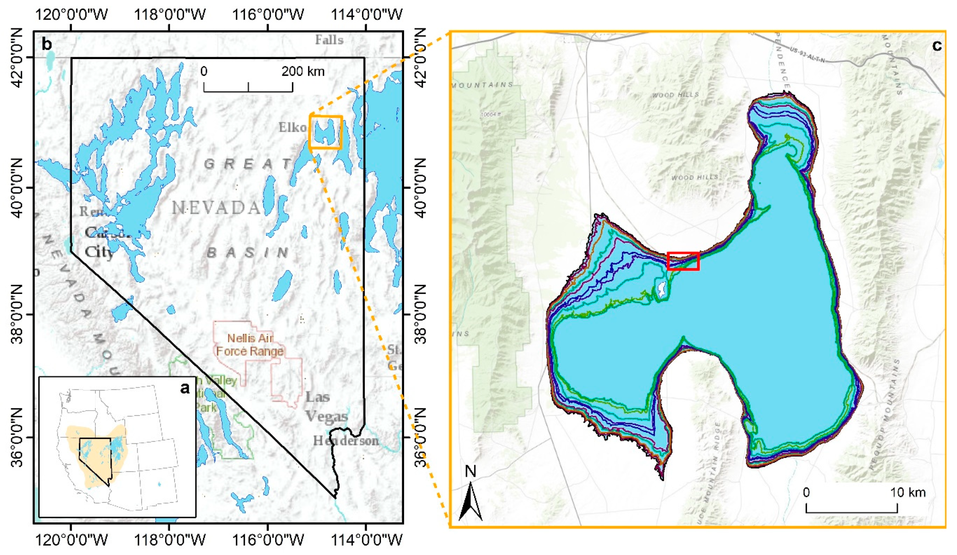
2.1. Setting

This project focused on shorelines built by pluvial Lake Clover, which occupied parts of the Clover and Independence Valleys in northeastern Nevada (Figure 1a,b) during the last glacial cycle. Age control provided by radiocarbon dating and luminescence techniques reveals that the lake reached its maximum extent (Figure 1b) ca. 17 ka BP [19,20] and Munroe et al. in review. At this time, Lake Clover had a depth of 20 m and covered 740 km² (Figure 1c). In contrast, permanent surface water is absent at low elevations in the Lake Clover watershed today, although some playas are seasonally flooded with shallow water sourced a snowmelt in the surrounding mountains [21].

Beach ridges constructed by Lake Clover are obvious topographic features that can be followed around the perimeter of the lake basin, often continuously for distances > 1 km (Figure 2). These ridges are typically ~1–2 m tall, feature broad relatively flat crests, and are steeper on their lakeward (downslope) side. Narrow, linear playas, typically with mud-cracked silty surfaces devoid of vegetation, are commonly present on the landward (upslope) side of ridges. These are presumably zones of deposition where the ridges act as dams impounding colluvium and slopewash.

Hand excavations reveal that these beach ridges are composed of coarse sandy gravel, locally imbricated, and interbedded with layers of pure sand (Figure 3a). Pockets and layers of silt are also common. In some deeper excavations, carbonate-cemented soil (caliche) or other indurated sediments were encountered ~100 cm below the ground surface.

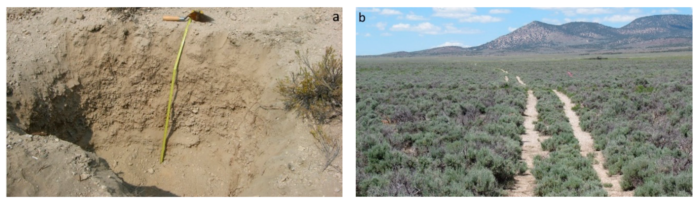
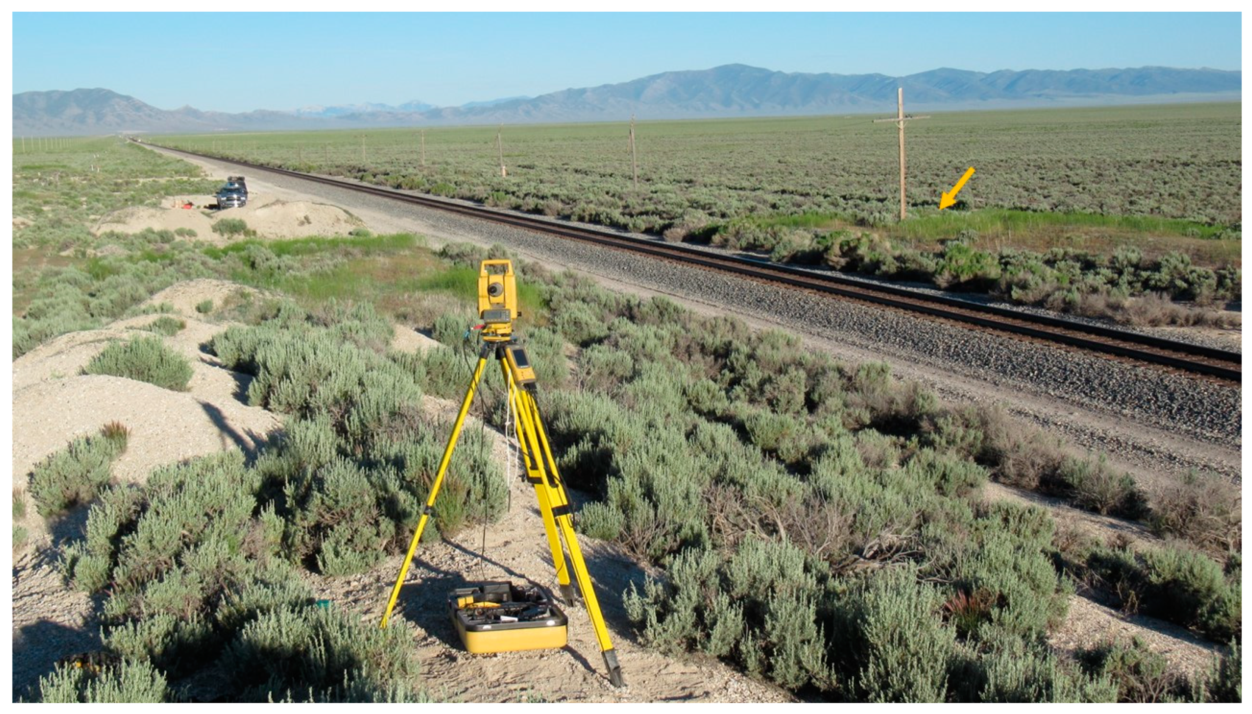
2.2. Field Methods

GPR data were collected along three transects crossing most of the preserved shorelines of Lake Clover. Transect locations were selected to follow existing jeep trails that provided linear routes clear of vegetation crossing the beach ridges at high angles (Figure 2 and Figure 3b). The highest transect, Transect A, crossed shorelines at 1725, 1724, 1723, 1721, and 1720 m. Transect B spanned the 1718 m shoreline. Transect C crossed the shorelines at 1715 and 1712 m. Two shorelines, at 1717 and 1713 m (orange in Figure 2), were not investigated with GPR because no linear route crossing over them through the sagebrush was available.

To constrain the topography of each transect, elevation data were measured with a Topcon GTS-235W total station every ~6 m along each transect (Figure 3b). The total station was first installed on an artificial height of land where the railroad line breaches the 1720 m beach ridge (Figure 2 and Figure 4). This point was used to survey Transects A and B. The total station was then moved 925 m to the southeast along the railroad line to survey Transect C (Figure 2). In both locations, the total station was referenced to a second class 0 vertical survey marker (Figure 2 and Figure 4). This marker (LQ0282) was installed by the Coast & Geodetic Survey in 1934, and has an estimated vertical error of +/− 5.6 cm. Position data for each measured point were exported as xyz coordinates relative to the total station, and processed to yield a topographic cross section along each GPR transect.

GPR data were collected along the three transects using an antenna with a central frequency of 400 MHz and a SIR-3000 controller manufactured by GSSI. Before data collection, the antenna was placed on the ground surface at the crest of the beach ridge and an automatic gain adjustment was conducted. The antenna was then returned to the uphill start of the transect and data were collected at a rate of 64 scans/second while the antenna and integrated receiver were towed at a slow walking pace along the survey line. In the vertical dimension, samples were collected at 512 samples/scan and 16 bits/sample. Marks were manually recorded in the GPR datafile when the antenna passed each of the points measured with the total station (Figure 3b). This approach allowed the resulting GPR transect to be georeferenced and topographically corrected. Transect were then resurveyed after a second auto-gain conducted with the antenna positioned on the fine silty sediments comprising the ground surface between the beach ridges. Given the contrasting behavior of radar waves in these two materials (coarse sandy gravel and fine silt), this approach supported the collection of separate sets of GPR data that collectively imaged all parts of each transect.

An average dielectric permittivity of the sediments underlying the studied transects was calculated at three locations where hand excavations encountered a prominent stratigraphic discontinuity at depth, along with an additional location where a natural exposure along an arroyo revealed a layer of caliche underlying the beach ridge at 1715 m (Figure 5). At all of these sites, the depth of the discontinuity was measured relative to the ground surface, and GPR data were collected on the crest of the beach ridge immediately surrounding the excavation (or the edge of the natural exposure). High-amplitude reflectors in the GPR data were correlated with the observed stratigraphy and measured depths of prominent stratigraphic contacts, and the dielectric permittivity was adjusted iteratively to align the GPR peaks with the appropriate depths. This approach yielded an overall average dielectric permittivity of 5.0 for these sediments, typical for dry quartz-rich sand [22].

2.3. Data Processing

The GPR data were processed in Radan 7.0. Steps included a time-zero correction to eliminate the impulse passing directly from the antenna to receiver (the direct wave); a full-pass background removal to remove the ground surface wave that can obscure shallow stratigraphy; various infinite impulse response (IIR) and finite impulse response (FIR) filters to remove low frequency noise; a 3-point range gain to amplify faint, deeper reflectors; distance and surface normalization (using points measured with the total station) to produce a scaled profile; and horizontal stacking to facilitate display of these long profiles on single pages. The average dielectric permittivity (5.0) determined for these materials (Figure 5) was used to convert two-way travel times to estimated depths below the surface.

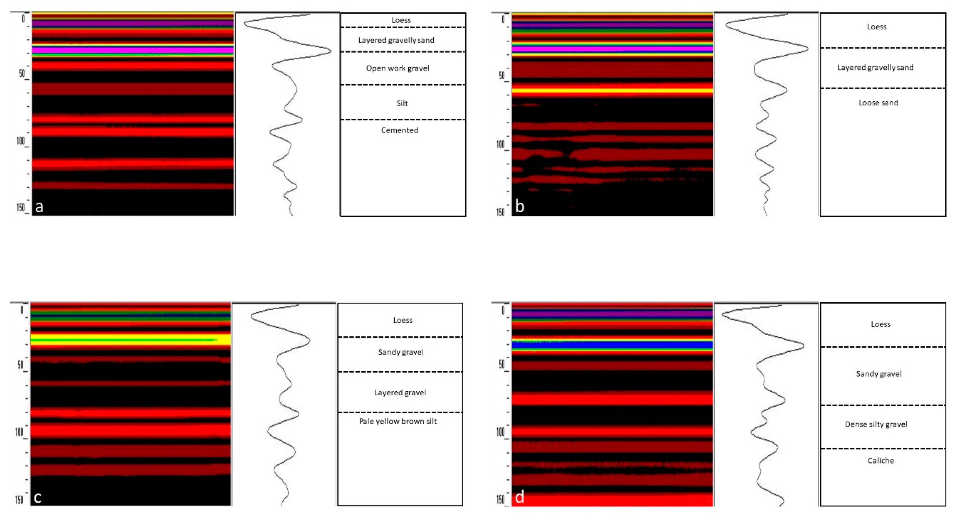
3. Results

GPR data were collected over a total linear distance of 1.1 km (Figure 2). Transect A, crossing the five highest shorelines of Lake Clover, extended for 512 m. Transect B over the 1718 m shoreline was 165 m long. Transect C, which crossed shorelines at 1715 and 1712 m, spanned 425 m. Using a dielectric permittivity of 5.0, interpretable radar data were obtained down to a depth of ~3 m. The depth of penetration was shallower between the shorelines, where fine silty sediments that impede EM transmission have accumulated on the upslope side of beach ridges. In these positions, near-surface sediments exhibit minimal contrasts in permittivity and typically returned weak, low-amplitude GPR signals. These sediment, therefore, appear only faintly stratified in the GPR data. In contrast, coarser sediments underlying the beach ridges offer strong permittivity contrasts resulting in numerous, high-amplitude reflections. Unlike the finer sediments, these beach gravels and sands are clearly resolvable as packages of stratified sediment.

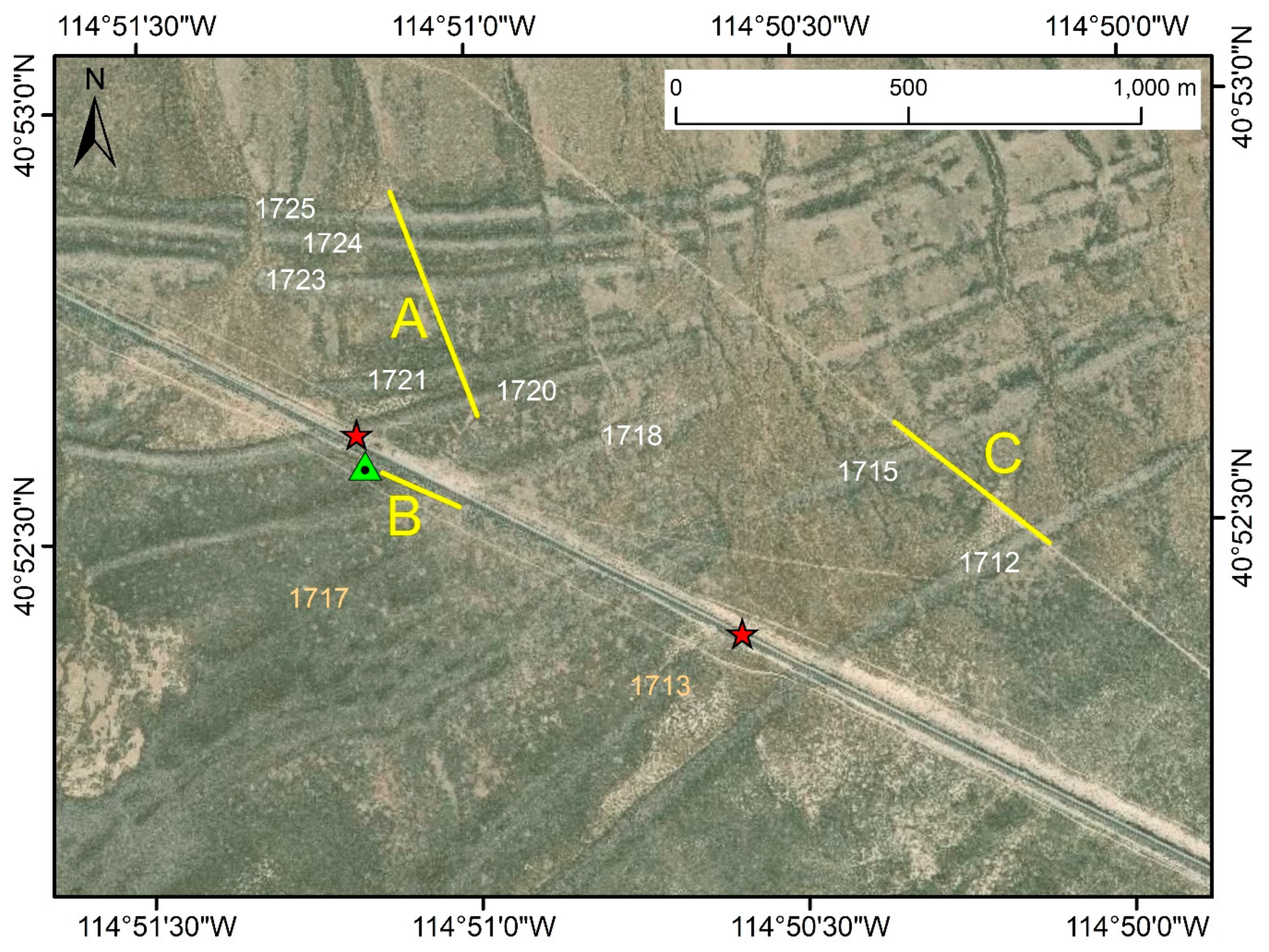
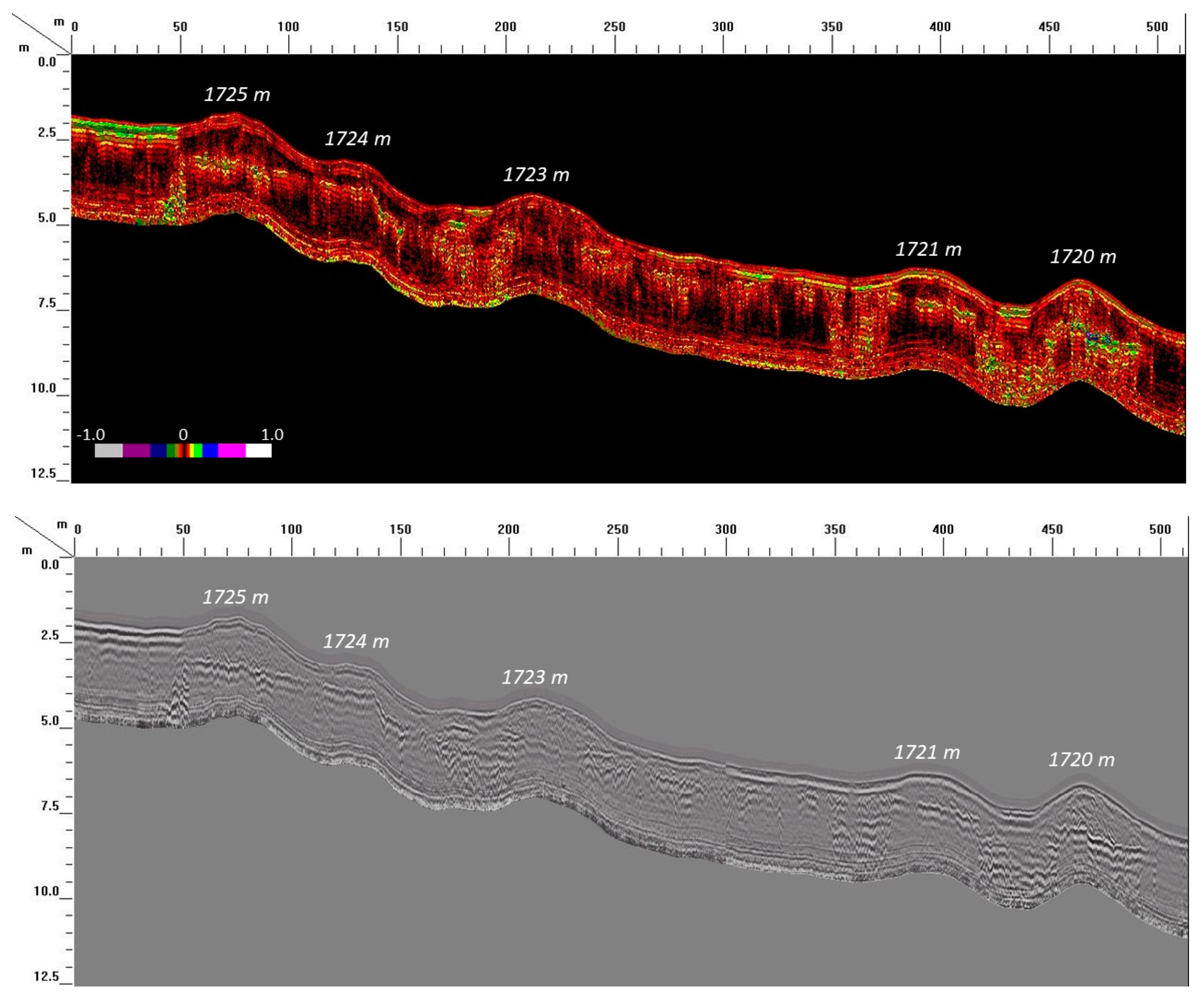
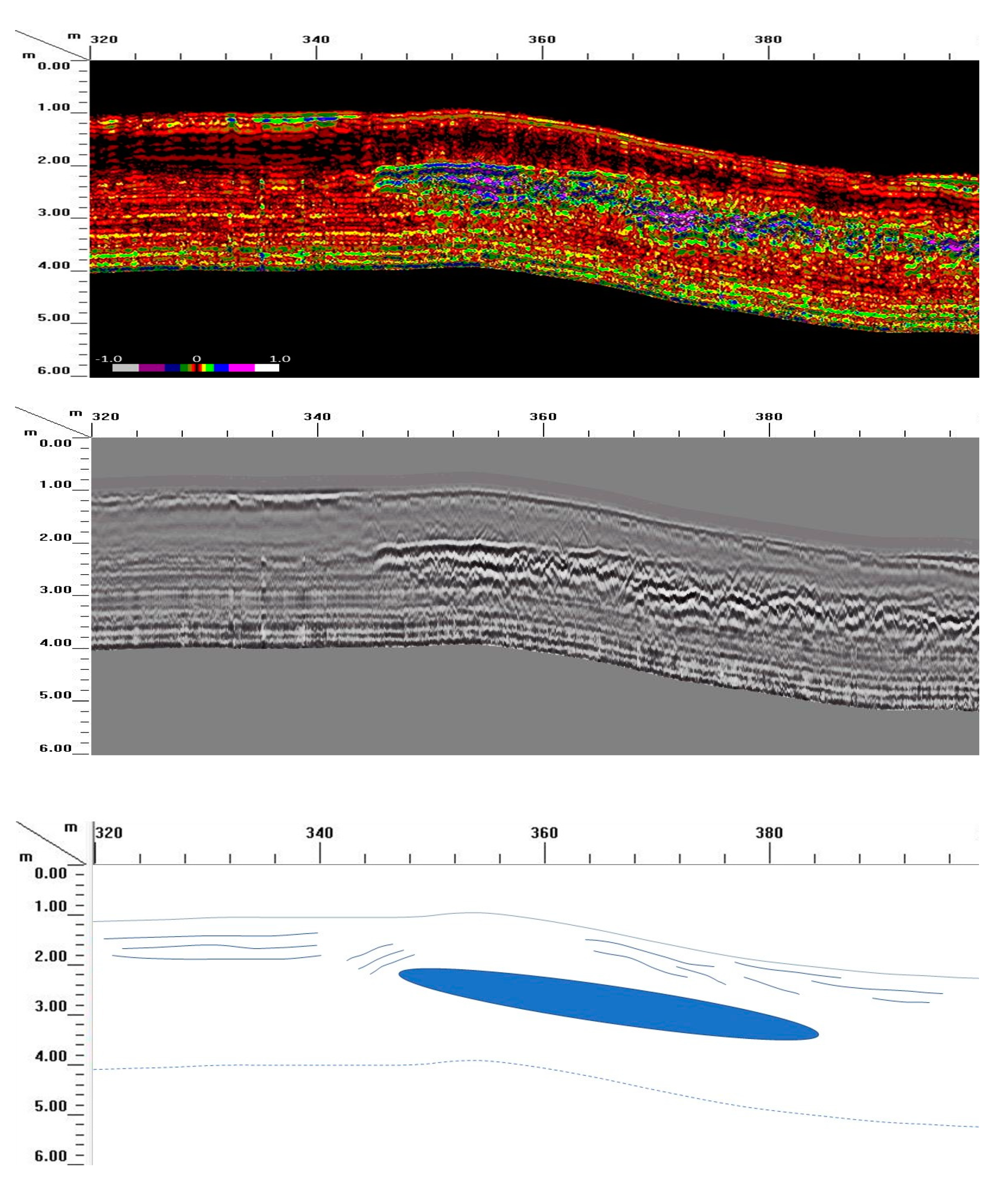
3.1. Transect A

The GPR data from Transect A (Figure 6) provide a detailed perspective on the highest five shorelines of Lake Clover. In this figure, and those that follow, the GPR data are presented with both a normalized color scale to accentuate contrasts and a traditional grayscale image to highlight structures. In all GPR profiles, landward is to the left and lakeward is to the right.

The upper two ridges crossed by Transect A, at 1725 and 1724 m, appear as a closely spaced pair of convex-upward sediment packages. In contrast, the shoreline at 1723 m is separate from the higher shorelines and has acted as a dam to impound a package of fine-grained sediments on the upslope side. The shoreline at 1721 is broad-crested and symmetrical. Finally, the 1720 m shoreline is notably prominent and sharp-crested. Stratified sediments are also impounded on the upslope side of the 1720 m shoreline

Particularly striking in Transect A is a laterally continuous, lakeward-dipping, high-amplitude reflector underlying all five of the shorelines (Figure 6). Also notable is a step-like offset in this reflector beneath the 1724 m shoreline. The origin of this feature is unclear, but it may be a fault scarp.

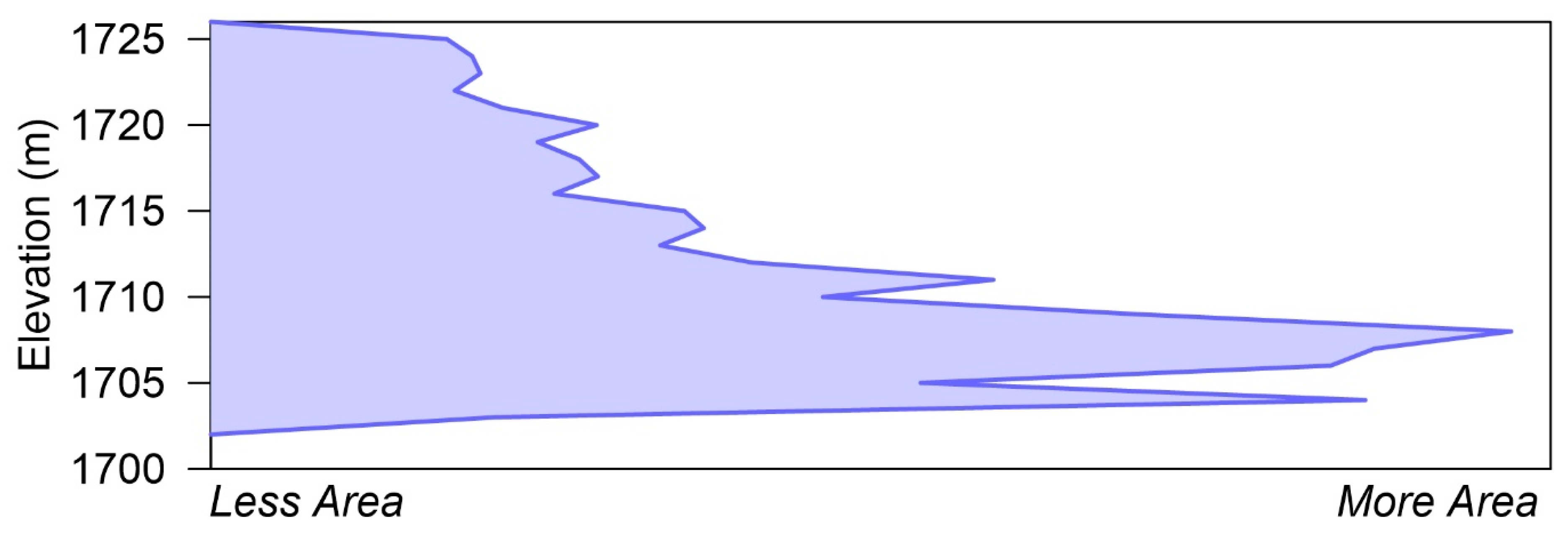
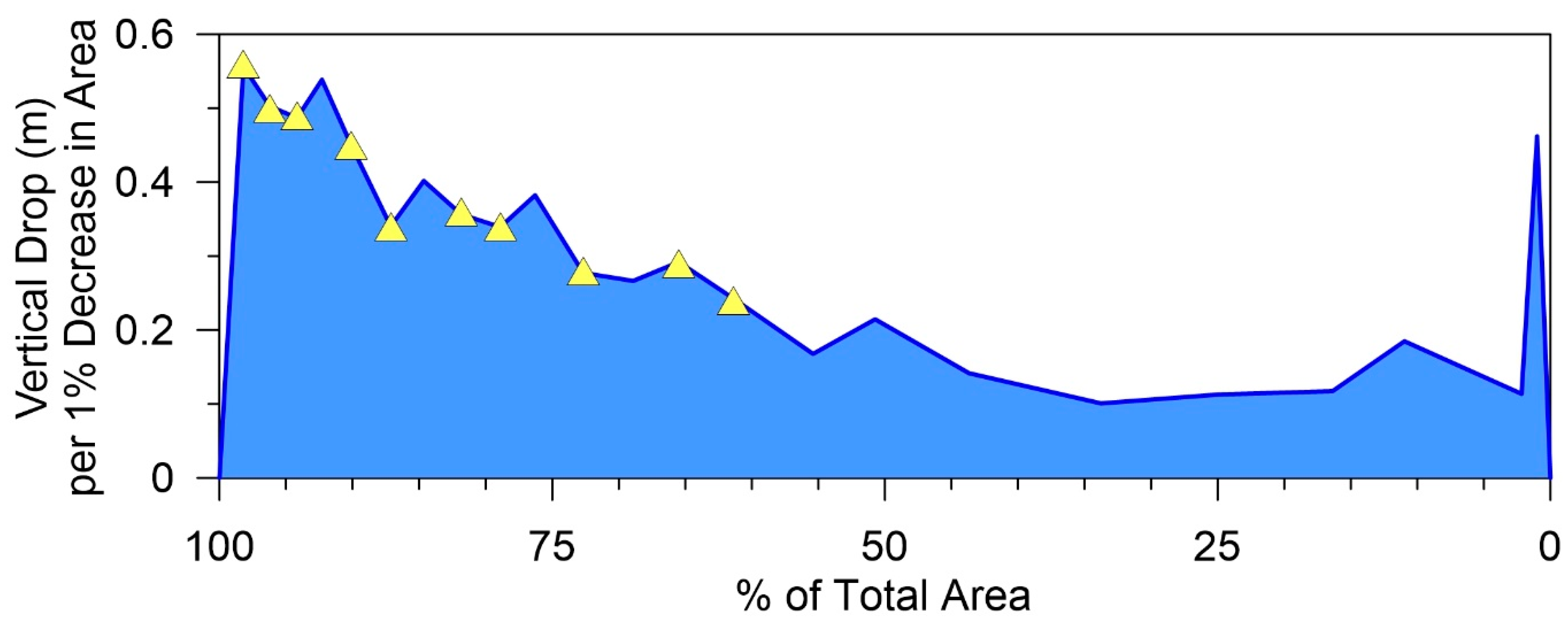
3.1.1. Shoreline at 1725 m

An enlargement of the GPR profile crossing the shoreline at 1725 m is presented in Figure 7. This ridge is the highest preserved feature built by Lake Clover, and was presumably constructed when the lake was at its maximum extent (Figure 1c). On the landward side of the shoreline, at a position of 50 m along the transect, a series of high-amplitude reflectors is present at and below a depth of ~3 m. The nature of these reflectors is unclear, however similar features are imaged beneath swales on the upslope side of both the 1723 and 1720 m shorelines (Figure 6). This pattern suggests that these reflectors may relate to sediment properties common to this landscape position, perhaps a greater accumulation of secondary carbonate (caliche) at depth beneath fine-grained sediments in swales.

The continuous, lakeward-dipping reflector underlying the shoreline forms a base for the sediments comprising the beach ridge (Figure 7). Hand excavations in this ridge encountered cemented material below a depth of ~75 cm, which likely corresponds to the continuous reflector underlying the entire GPR profile.

Lakeward from the ridge crest, the internal stratigraphy of the beach ridge consists of a series of lakeward-dipping reflectors, each spanning ~2 m horizontally (Figure 7). Hand excavations confirm that these are layers of gravelly sand interbedded with open-work gravel. In some cases, such as near 95 m along the transect, these features clearly downlap onto the continuous reflector underlying the entire shoreline.

The stratigraphy between ~57 and 72 m along the transect contains strata that dip lakeward on the right side, and landward on the left side (Figure 7). Although the 3-D shape of this package of sediment cannot be fully interpreted from a 2-D profile, this may be a buried portion of the original beach berm produced by Lake Clover at this elevation.

3.1.2. Shoreline at 1724 m

A GPR cross section and interpretation through the shoreline at 1724 m is presented in Figure 8. Here the continuous, lakeward-dipping reflector is again prominent below the sediment comprising the beach berm. Notably, the steepness of this reflector increases abruptly between 138 and 143 m along the transect. In the less shortened profile shown in Figure 8 this steepening is less abrupt than it appears in Figure 6. Nonetheless, the overall consistent slope of this feature does change at this position.

To the right of this local steepening, strata arranged in lakeward-dipping packages that downlap onto the underlying reflector are visible, particularly at ~145 m along the transect (Figure 8). Additional inclined reflectors are resolvable farther to the right. Overall, the broad crest of this shoreline spans from ~120 to 140 m, with a maximum sediment thickness (70 cm) at a position of ~132 m. Shoreline sediments exceed this thickness ca. 144 m lakeward of the local steepening in the basal reflector, but at the surface this position corresponds with the beach face rather than the berm crest.

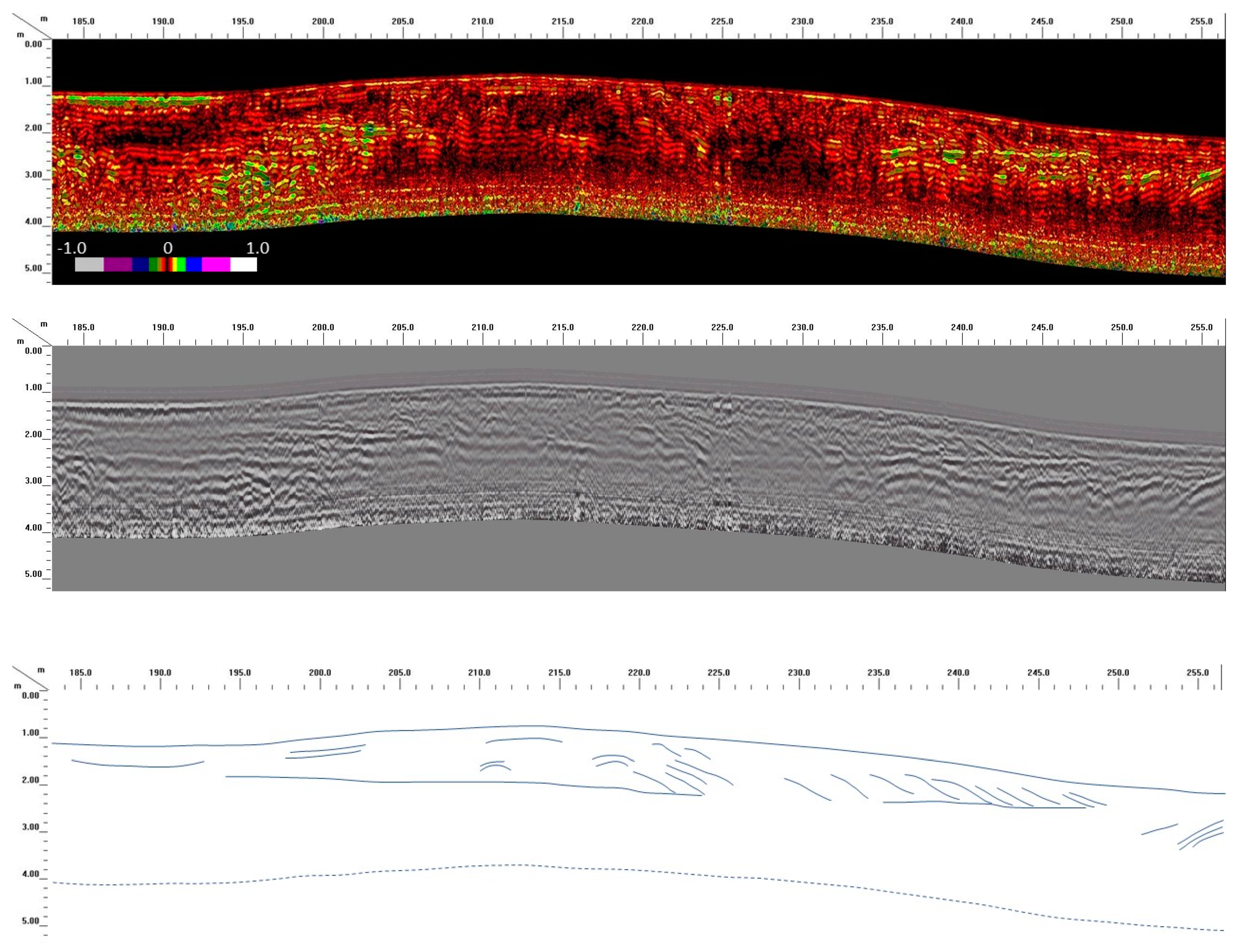
3.1.3. Shoreline at 1723 m

Figure 9 presents a GPR profile and interpretation crossing the shoreline at 1723 m. Here the continuous underlying reflector is again clearly visible, particularly between 197 and 247 m. Toward the left end of the profile, between 183 and 193 m, flat-lying strata with a prominent reflector near the surface are present. On the basis of observations made during the acquisition of GPR data, these are fine-grained (silty) sediments that have accumulated on the upslope side of the shoreline after ridge formation. At greater depths, particularly around 190 m along the transect, little radar energy was returned from these sediment, consistent with uniform silty materials.

At ~200 m along the transect, reflectors that dip shallowly in a landward direction are present (Figure 9). These are likely overwash deposits emplaced by storm waves that crested over the ridge when the lake stood at 1723 m.

The sediments comprising this shoreline reach a maximum thickness of 125 cm at ~220 m along the transect. A hand excavation elsewhere along the crest of this feature, not at the same location where the GPR data were acquired, penetrated gravelly sand transitioning to loose sand at depth of 55 cm with an abrupt contact to cemented sand at 80 cm.

Between 220 and 250 m along the transect, the sediments beneath the former beach face are clearly resolvable as a series of lakeward-dipping reflectors exhibiting downlap onto the underlying continuous reflector (Figure 9). A local high-amplitude reflector is present at a shallow depth at 225 m along the transect. The significance of this feature is unclear.

Finally, at the extreme right side of Figure 9, reflectors that dip steeply in a landward direction are visible at a position of 252-255 m. These reflectors are buried beneath ~1 m of lakeward-dipping strata that are likely distal components of the overall beach ridge. The steep, landward features, therefore, predate formation of the beach ridge. Their significance is also unclear.

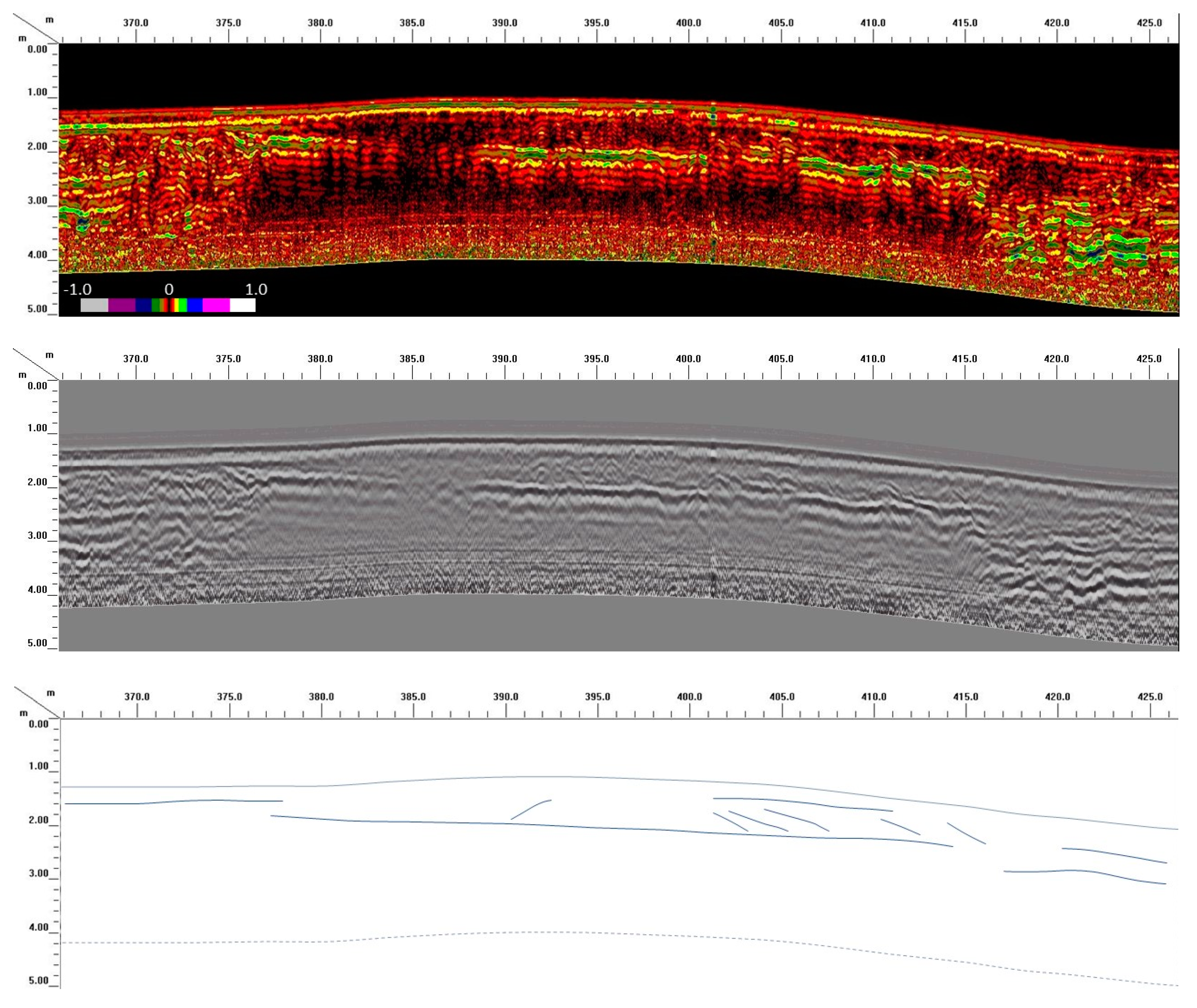
3.1.4. Shoreline at 1721 m

A GPR transect and interpretation crossing the shoreline at 1721 m are presented in Figure 10. Here the GPR data on either side of the ridge exhibit multiple high-amplitude reflectors at depth, particularly to the left of 376 m and to the right of 418 m. On the left side, these reflectors reach almost to the ground surface, whereas on the right they start at a depth of ~1 m. In between these zones, a continuous lakeward-dipping reflector is clear. This reflector appears broken around 385 m along the transect, but this is likely a shadow zone created by locally greater reflection of the EM pulse in the near surface stratigraphy at this location.

Centered below 395 m is a narrow (~5 m wide) package of sediment delineated by opposing landward dipping (left side) and lakeward-dipping (right side) reflectors (Figure 10). Similar to the 1725 m shoreline (Figure 7) this may represent a buried berm at the core of the overall beach ridge, although some of the landward-dipping reflectors may be hyperbolic reflector tails associated with point reflectors in the beach ridge interior. Lakeward from this position, particularly between 400 and 415 m along the transect, numerous lakeward-dipping reflectors are visible downlapping onto the underlying continuous reflector.

3.1.5. Shoreline at 1720 m

The GPR transect through the lowest shoreline in Transect A, at 1720 m, is presented in Figure 11. Landward (left) of ~450 m along the transect, the GPR data reveal generally horizontal, parallel reflectors to a depth of ~2 m below the ground surface. In contrast, beneath the main body of the beach ridge, reflectors dip landward on the upslope side of the ridge crest, and lakeward on the downslope side.

Similar to the 1725 and 1721 m shorelines (Figure 7 and Figure 10), a small area of symmetrical right- and left-dipping reflectors defines a buried berm at the core of the shoreline between 462 and 466 m (Figure 11). Lakeward from this point, dipping reflectors exhibit a downlapping relationship with the underlying continuous reflector to ~480 m along the transect.

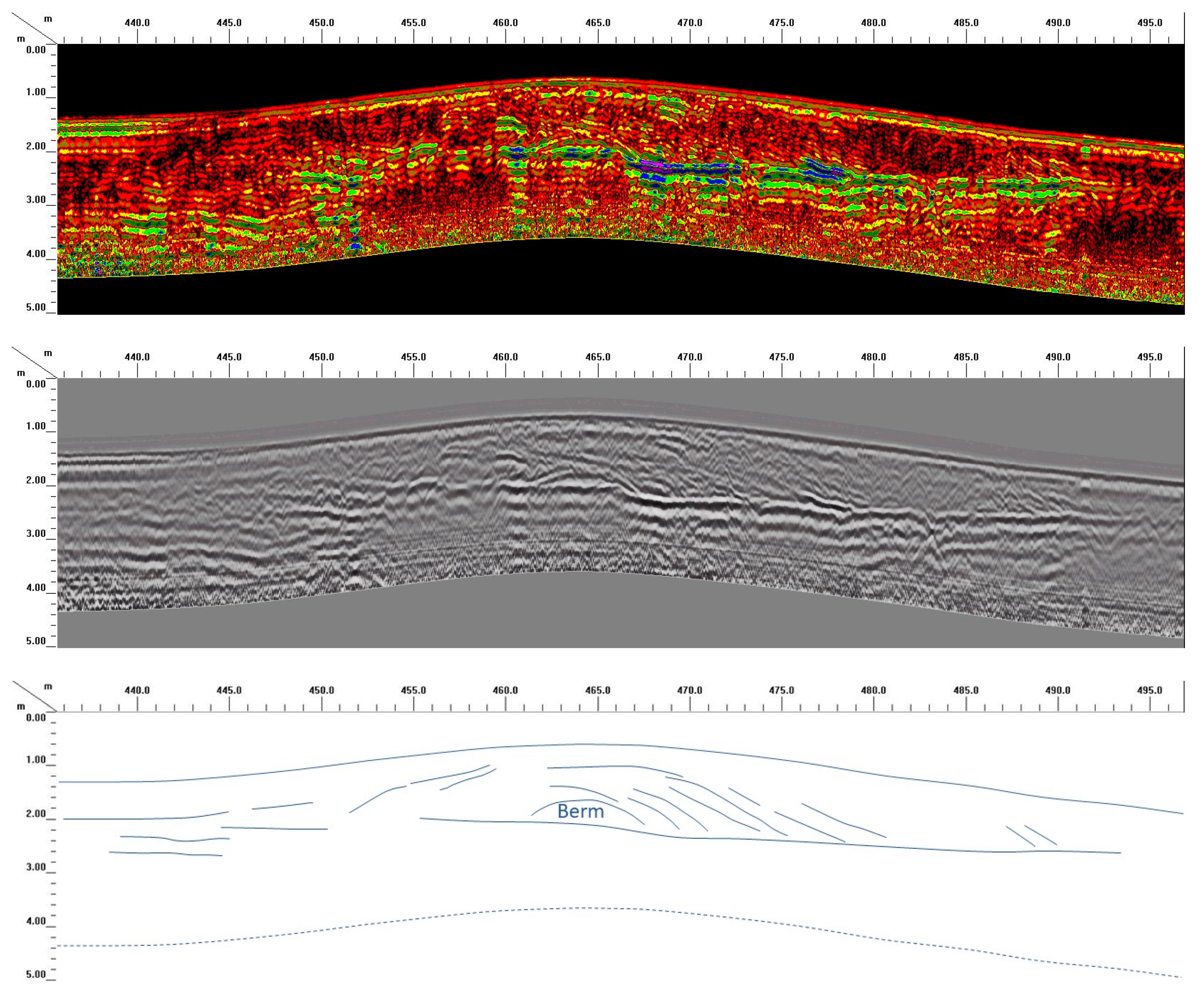
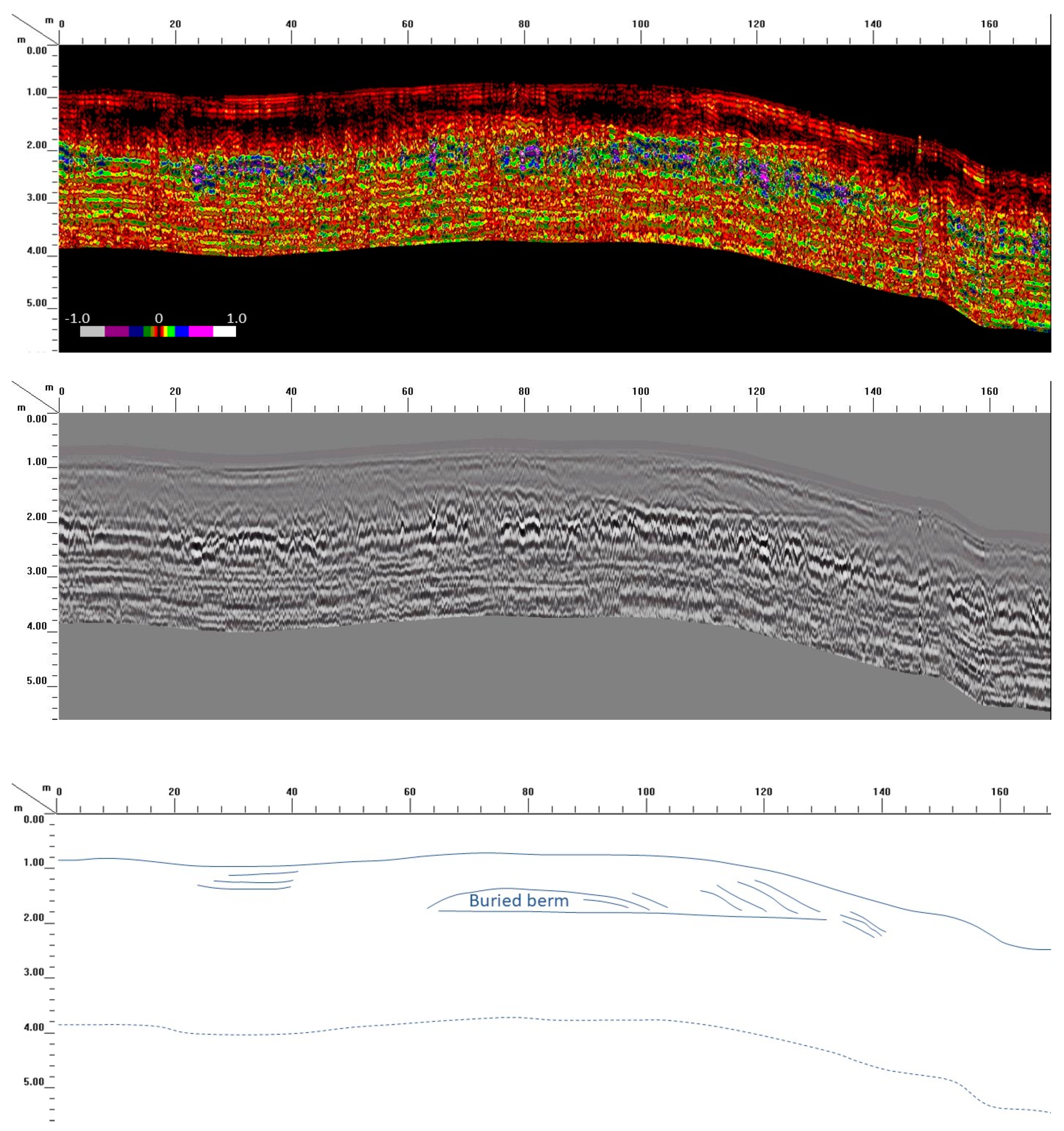
3.2. Transect B

Transect B crossed just a single shoreline, at 1718 m. This broad feature was investigated on the south side of the railroad line, in contrast with the other shorelines, because that was the only place where a jeep trail provided a suitable route through the dense sagebrush vegetation (Figure 2).

Shoreline at 1718 m

The GPR transect crossing the shoreline at 1718 m is presented in Figure 12. Here the continuous reflector underlying the shoreline sediment is less obvious than in Transect A (Figure 6), but it is still discernable, particularly between ~100 and 130 m. To the right of 130 m, this reflector is difficult to trace, but it may step down to a greater depth similar to the offset beneath the shoreline at 1724 m (Figure 8).

Between ~65 and 100 m along the transect is a package of sediment defined by inclined reflectors dipping lakeward on the right side and landward on the left (Figure 12). This appears to be an older shoreline buried at the core of the larger beach berm. The crest of the overall ridge is offset to the right (lakeward) from the crest of this buried feature by ~30 m. To the left (landward) of this buried berm, the sediments above the basal reflector reach a maximum thickness of ~100 cm. Faint subhorizontal stratigraphy is resolvable within these deposits (Figure 12). This layering, combined with observations made during acquisition of the GPR data, support the interpretation that this sediment is colluvium that accumulated on the upslope side of the beach ridge.

Farther to the right, particularly at a position of ~120 m along the transect, packages of lakeward-dipping reflectors are visible that downlap onto the underlying continuous reflector (Figure 12). Notably, near the 140 m mark, several of these reflectors are resolvable at a greater depth, following the apparent downward step in the basal reflector.

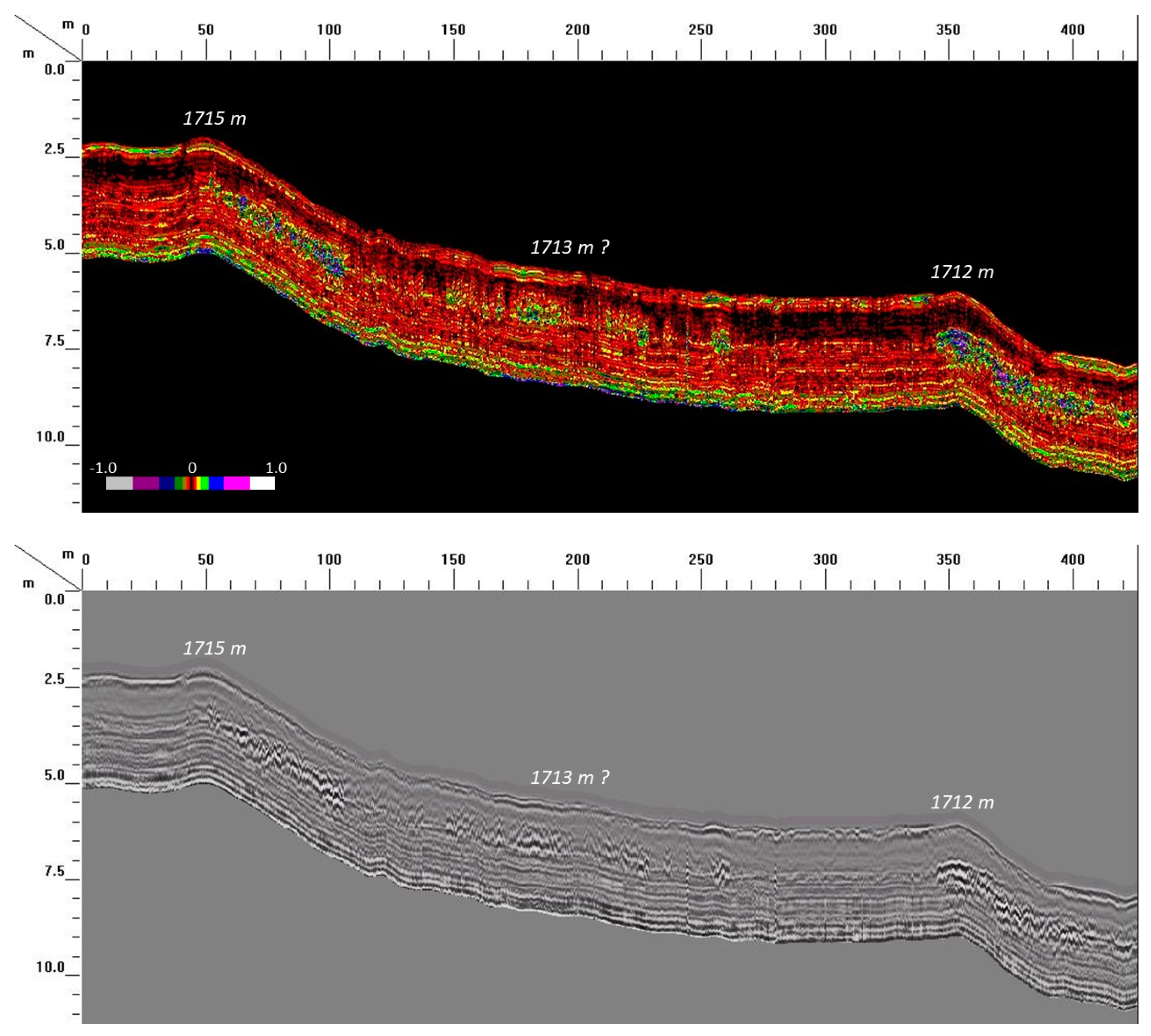
3.3. Transect C

Transect C crossed the lowest three shorelines produced by Lake Clover at 1715, 1713, and 1712 (Figure 13). Only the 1715 and 1712 m shorelines are present as positive topographic features at this location; the 1713 m shoreline is missing, either because it was eroded away or buried by younger sediment. In the GPR data, high amplitude reflectors are present (marked by “1713 m ?” in Figure 13), particularly around 180–200 m, which may represent buried portions of the missing 1713 m berm.

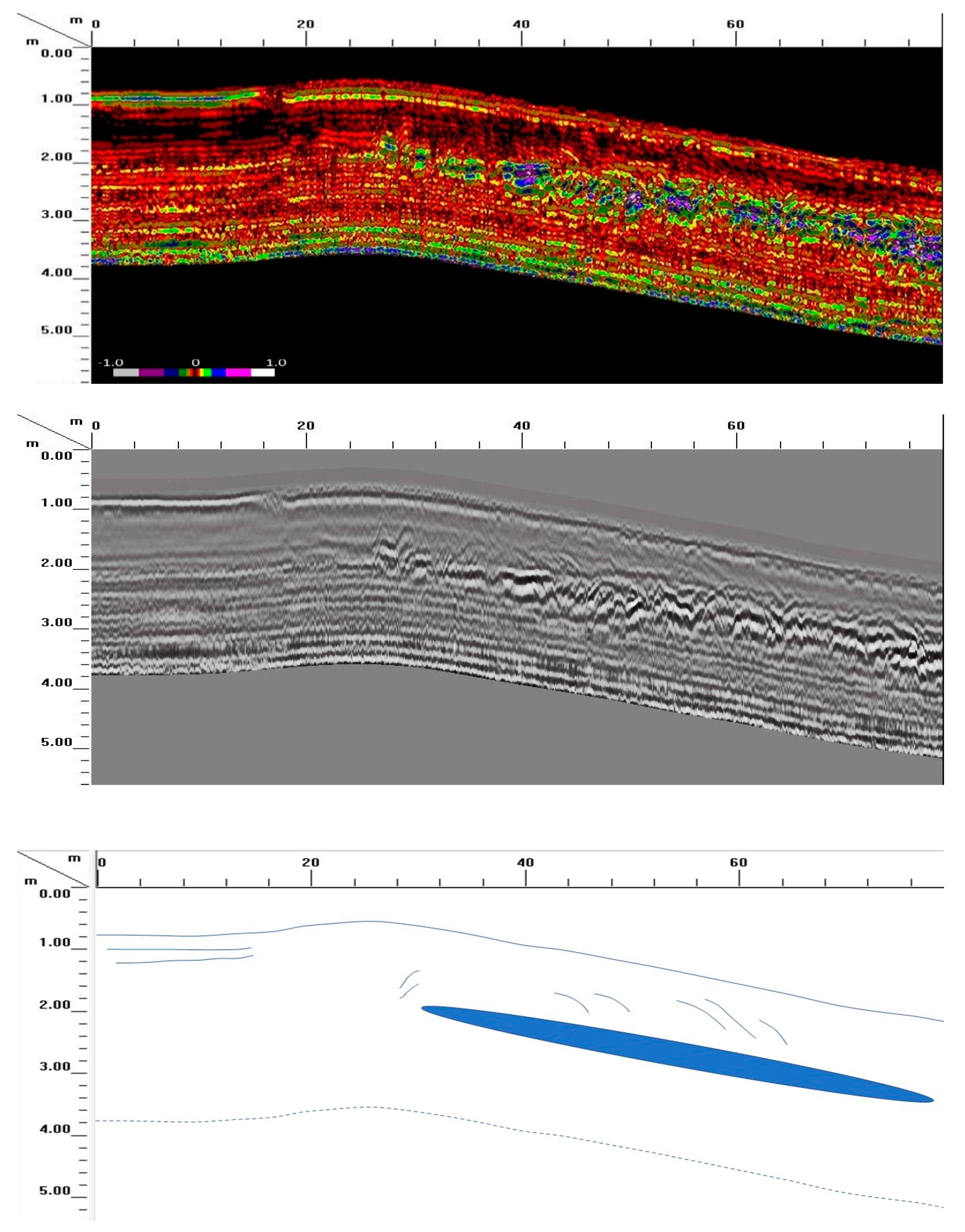
3.3.1. Shoreline at 1715 m

The GPR transect crossing the shoreline at 1715 m is presented in Figure 14. A meter-thick package of faintly stratified sediment is present on the landward (left) side of the ridge crest. A notably strong reflector, perhaps a cemented layer in the soil profile or a contact between older beach-related sediments and younger overlying loess, is continuous for the first ~15 m along the transect.

The ridge itself is a convex-up package of stratified sediments, the form of which is conformable with the overall shape of the beach ridge (Figure 14). Farther to the right, particularly between ~45 and 60 m along the transect, steep, lakeward-dipping reflectors are visible.

Beneath these reflectors, extending from ~30 m to the end of the transect at ~80 m, is a diffuse zone of high-amplitude reflectors, dipping lakeward with a slope matching the overall ground surface (Figure 14). A natural exposure along an arroyo cut across the 1715 m shoreline reveals the presence of caliche at a depth of 80–100 cm below the ground surface (Figure 5). Presumably this layer of caliche extends beneath the entire GPR profile. However, the strong near-surface reflectors from 0–30 m blocked much of the EM pulse, rendering the deeper stratigraphy unresolvable.

3.3.2. Shoreline at 1712 m

Figure 15 presents the GPR transect across the lowest preserved shoreline of Lake Clover, at an elevation of 1712 m. When this ridge was constructed, Lake Clover covered ~485 km² (a decrease of 35% from its highstand area) and had a maximum depth of ~9 m. Similar to the shoreline at 1715 m (Figure 14), a package of faintly stratified sediment is present on the upslope side of the ridge crest. This material contains a strong near-surface reflector that apparently limits the penetration of EM in this part of the transect.

The ridge crest itself, located at ~30 m along the transect, is underlain at a depth of ~110 cm by notably high-amplitude reflectors that continue lakeward at progressively lower elevations (Figure 15). Given observations made in the exposure through the ridge at 1715 m (Figure 5), this material is likely caliche. Apparent absence of this reflector to the left of 20 m can be explained by blocking of the EM signal by the strong reflector in the near-surface.

The rate at which the high-amplitude reflector appears to descend is more gradual than the slope of the ground surface. As a result, the sediment package forming the former beach face thins in the lakeward direction. Lakeward-dipping strata are resolvable within these beach face sediments, particularly between 50 and 60 m along the transect (Figure 15).

4. Discussion

4.1. Common Features of the GPR Profiles

Interpretation of the GPR transect collected across shorelines of pluvial Lake Clover reveals several features that are consistent between many, if not all, of the ridges. First, all ridges are comprised of convex-upward sedimentary packages sitting atop a lakeward-dipping, high-amplitude reflector. Many hand excavations into the crests of individual beach ridges encountered a carbonate-cemented horizon at depth; at four sites the depth of this horizon was used to determine the dielectric permittivity of these materials (Figure 5). The apparent slope of this reflector is 0.0126 (dropping 5.5 m over 437 m), matching the gradient of the alluvial fan surface upslope from the highest shoreline. This correspondence suggests that the reflector is the original land surface upon which the shorelines were constructed, or a layer of caliche that formed within the soil profile on the former landscape. Beach ridges are clearly resolved as accumulations of sand and gravel concentrated by wave action at the point where the waters of Lake Clover met this pre-lake landscape.

Second, all of the GPR profiles contain packages of lakeward-dipping strata beneath the former beach face. On the basis of observations made in hand excavations into the beach ridge sediments, these are likely layers of gravelly sand interbedded with more sand-dominated sediment. Together these materials are typical of a wave-washed, high-energy environment and are similar to those reported from other pluvial lake shorelines in the Great Basin [11,16,23].

Third, some GPR profiles reveal packages of landward dipping reflectors beneath the landward side of the beach crest. These are presumably overwash deposits emplaced by storm waves that overran the beach crest and transported sediment to the landward side of the shoreline [18].

Fourth, no beach ridges contain evidence of erosional unconformities or depositional hiatuses that would suggest submergence by later high water after ridge formation. Although this is negative evidence, it is consistent with sequential ridge formation during overall lake regression.

Finally, many of the ridges contain, at their core, a package of sediment distinguished by opposing lakeward and shoreward-dipping reflectors. In cross section, these packages mimic the overall convex-upward shape of the larger beach ridge and appear to be proto-beach berms that were buried by later sedimentation [18]. In all cases, the crests of these buried berms are located landward from the crest of the overall beach ridge, indicating a lakeward shift in focused sediment deposition during beach ridge growth.

4.2. Model for Beach Ridge Construction

Studies of beaches built by other pluvial lakes, as well as the modern Laurentian Great Lakes, support a model of the events responsible for the construction of beach ridges like those produced by Lake Clover. Formation of a beach ridge as a preservable landform with positive relief is dependent on the rate of change of water level and the availability of sediment in the near-shore system [24,25]. In the case of Lake Clover, it is unlikely that sediment supply varied significantly during the episode of beach construction; there are no lakes upstream that would have altered the amount of sediment reaching Lake Clover, glaciers in the Lake Clover watershed were restricted in extent, and no large rivers entered the lake that could have impacted the delivery of sediment to the near-shore system. Instead, variations in the rate of water level change were likely the more important variable in the formation of these beaches.

When the rate of change of water level is zero (or near zero) and the water level is stable (or nearly stable), then the repeated action of waves will winnow fines and concentrate coarse sediment at the water’s edge [25]. Slow rise of the water level, matched by an increase in sediment supply, will cause this shoreline sediment to aggrade vertically forming a beach ridge. However, if the water level rises too quickly, then the beach ridge will be submerged, and a new ridge will be built at a higher elevation farther up the slope. In contrast, continued stability or slow rates of water level fall result in progradation of the shoreline in a lakeward direction as additional material is added incrementally to the beach face [18]. More rapid rates of water level fall can exceed the ability of the waves to concentrate material at a particular location. Beach sediment will, therefore, be distributed uniformly across the slope as the water retreats to a lower elevation. If the water level stabilizes again, a new beach ridge will be constructed farther downslope [25].

This general model of beach ridge formation fits neatly with the evidence from Lake Clover. The buried berms imaged at the core of many of the beach ridges represent the first concentration of material produced when the regressing lake paused at a particular elevation (or, in the case of the highstand shoreline, when that elevation was first reached). Stability of the water level, or even slight water level rise, drove slight upward aggradation that buried these original berms. Overwash resulting from particularly large storm waves further buried these berms by transporting material up and over to the landward side. Continued water level stability, or perhaps water level fall at a slow rate, caused the shoreline to prograde lakeward, building the series of lakeward-dipping reflectors beneath the beach face that were observed in all shorelines [18]. Eventually, accelerating water level fall, perhaps combined with changes in the availability of sediment, terminated formation of a particular shoreline as the water level descended faster than shoreline construction could proceed. Resumed stability (or a reduced rate of regression) of the water level at a new, lower elevation, then initiated another cycle of (1) initial berm construction, (2) aggradation and burial, (3) followed by lakeward progradation, and 4) eventual abandonment. The sequence of shorelines seen in the study area indicates that this overall pattern was repeated multiple times during the regression of Lake Clover.

Exactly how long the water level must remain stable in order to construct a preservable shoreline at a certain elevation is unclear. However, it is worth noting that beach berms were built by the modern Great Salt Lake in Utah in response to just a few years of high water in the 1980s [26,27]. Thus, the Lake Clover beach berms do not necessarily imply stability of lake level over long (>>~10¹ year) time intervals.

4.3. Implications for Relative Age and Paleoclimate Conditions during Beach Ridge Formation

The beach ridges built by pluvial Lake Clover are unequivocal evidence for profound hydroclimate change. As such, determining when they were constructed, and how hydroclimate conditions evolved during the episode of beach formation, are important objectives in better understanding the paleoclimate history of this region. As noted above, the internal stratigraphy of the ridges, combined with the lack of evidence for submersion and erosion, are best explained by ridge formation in response to monotonic lake regression. In other words, in terms of relative age, Lake Clover built its highest shoreline first, then constructed sequentially lower shorelines step by step until the lake disappeared or became too small to support the wave energy necessary to construct preservable shoreline landforms. This model implies that the overall peak in effective moisture responsible for the Lake Clover highstand was followed by a decrease in effective moisture and increasing aridity that shrank the lake before eliminating it entirely.

Absolute age control helps to put this history of Lake Clover into a chronologic context. Five radiocarbon dates are available for gastropod shells obtained from two different locations along the highstand shoreline of Lake Clover. These ages fall into two non-overlapping clusters, one with calibrated ages ca. 19.5 ka and another ca. 17 ka BP [20]. The simplest, although surprising, interpretation of these ages is that the lake coincidentally reached its highstand elevation twice during the last glacial cycle; the highstand shoreline, therefore, is a compound feature. On the other hand, no evidence was noted in the GPR profile across the highstand ridge to suggest that this feature was built in stages by separate episodes of high water (Figure 7). A buried berm is present at the core of the highstand beach ridge, and it is possible that this feature represents the older episode of highwater at this elevation. However, buried berms are present at the core of several other ridges, and it is unlikely that they are all compound features. The gastropod shells yielding the two clusters of radiocarbon ages were collected from different sites, and all of the older samples came from a greater depth below the surface. This correspondence raises the possibility that the older shells were obtained from sediments that stratigraphically pre-date the ridge built at 17 ka BP. Future GPR work focused on the location where these radiocarbon ages were obtained could clarify whether the older ages reflect an older landform buried beneath the highstand shoreline.

Other information about the absolute ages of the Lake Clover shorelines is provided by luminescence dating of quartz and K-feldspar sand grains collected from pits excavated into beach ridge crests in the immediate vicinity of the GPR transects [19] and Munroe et al. in review. These results confirm an age of 16–17 ka BP for the highstand ridge, document regression of the lake over several thousand years in the latest Pleistocene, and reveal that the lowest shoreline was constructed in the earliest Holocene.

Previous work has proposed a variety of mechanisms for the increased effective moisture in the Great Basin that drove pluvial lakes to their late Pleistocene highstands. Whether this moisture was a response to southward deflection of the prevailing storm track by the Laurentide Ice Sheet [28,29,30], steering of storms inland from the Pacific [31], or even a response to northward moisture transport [32], remains a topic of debate. What is clear, however, is the synchrony of many lake highstands across the entire latitudinal sweep of the Great Basin with Heinrich Stadial I (H1) in the North Atlantic region [20,23]. H1 was a massive release of icebergs from the Laurentide Ice Sheet, which drove dramatic millennial-scale climate changes of at least hemispheric extent [33,34]. Melting of these icebergs apparently altered ocean currents in the North Atlantic [35], leading to cooling of near-surface waters [36] and tremendous sea-ice expansion [37]. Farther afield, these changes impacted the average position of the Aleutian Low in the northern Pacific [38], which helped to steer moisture into the southwestern US [39]. As a result, effective moisture increased rapidly in the Great Basin in response to H1, and pluvial lakes quickly expanded to larger surface areas in equilibrium with a wetter climate.

Together the combination of luminescence age results with the GPR profiles reveals just how unusual the moisture pulse associated with H1 was: after spiking rapidly to its highstand elevation, Lake Clover steadily regressed as the climate transitioned into the aridity that characterized the Holocene. Aside from the somewhat equivocal cluster of older radiocarbon dates, there is no stratigraphic, geophysical, or geomorphic evidence to suggest that Lake Clover was near its highstand elevation multiple times. There is evidence that some pluvial lakes were high during other glacial cycles of the Pleistocene [4,40], however these may also have been driven by teleconnections with the North Atlantic [41,42]. Either way, the late Pleistocene highstand of Lake Clover and the lower shorelines are, therefore, not the result of repeated climatic fluctuations that alternatingly drove the lake to higher and lower elevations, building, submerging, and re-exposing beach ridges during multiple transgressions and regressions. Rather, the rise of the lake to its highstand was an unusual, perhaps singular event (at least in the context of the last glacial cycle), that was followed by a long interval of lake regression.

At the same time, the presence of shorelines below the highstand ridge does indicate that the rate of water-level lowering slowed or stopped multiple times during overall regression. One possible explanation for that behavior is that the overall transition toward greater aridity after Heinrich Stadial I was not steady, and that conditions occasionally stabilized long enough for water balance of the lake to come into equilibrium. Support for this theory comes from luminescence ages indicating that after regressing rapidly into the warm Bølling/Allerød interval, Lake Clover built some of its lower shorelines during the cooler Younger Dryas stadial [19] and Munroe et al. in review.

On the other hand, the presence of shorelines does not necessarily require that a climatic change temporarily stalled the desiccation of the lake and held the water level at a constant elevation. Figure 16 illustrates that that the area-altitude distribution beneath the highstand beach ridge is not uniform. Rather, there are inflections and irregularities that would have altered the rate at which the water level was falling even if lake area was steadily decreasing. Therefore, even if the reduction of the lake surface area proceeded at a constant rate in response to climate forcing, the rate of water level fall could still have varied due to the hypsometry of the basin.

This analysis is furthered by determining the vertical lowering of the water surface that would have accompanied each increment of area loss (in vertical m/1% of total lake area). In Figure 17 the result of this calculation is presented, and the position of the mapped shorelines is highlighted. This analysis is somewhat circular, since the hypsometry of the basin is calculated from the modern topography where the shorelines are present. Nonetheless, most beach ridges are clearly associated with reduced rates of water-level fall. Local accelerations in the rate of water-level lowering, reflecting elevation bands through which the water-level would have lowered more rapidly, tend to occur between the preserved shorelines. The salient conclusion is that recessional shorelines could have been constructed at times when the rate of water-level lowering slowed in response to the overall shape of the lake basin. The presence of these shorelines may certainly reflect a climatic cause, but this is not the only possible explanation.

4.4. Limitations and Directions for Further Research

The GPR data collected in this project provide valuable information about the subsurface stratigraphy of these beach ridges, information that could otherwise be attained only through expensive excavations. Nonetheless, there are some clear limitations to these data that should be considered, some of which provide useful guidelines for planning similar projects in the future.

One limitation is that the depth estimates for contacts and other features seen in the GPR data are entirely dependent on the assumed value of dielectric permittivity. This value was derived from GPR data acquired over prominent stratigraphic contacts with known depths at a few representative locations (Figure 5), so it is likely reasonable for this study area. However, because the properties of the surveyed sediments vary along each GPR transect, ranging from dense silt to loose gravelly sand, application of a single dielectric value for all the GPR data introduces error into the depth estimates. Future work, perhaps involving mechanical augering to add ground truth from other locations, could help refine the assumed dielectric value. If it is demonstrated that the dielectric permittivity varies greatly between the silty sediments and the material comprising the ridges, then it might be better to present each transect in subsections, each with its own dielectric value, rather than applying a single value to the entire dataset.

Second, the GPR data are inherently 2-dimensional, because they were collected as transects oriented roughly normal to the beach ridges. True dip of subsurface reflectors cannot be determined from a single 2-D cross section. As a result, the direction of dip (for instance, lakeward) is constrainable, but the actual magnitude of the dip is not. Future work could employ 3-D techniques [16,43] to gain additional understanding of how inclined packages of sand and gravel are arranged beneath a beach face.

Finally, a familiar challenge in GPR studies is the reality that the central frequency of the selected antenna controls the depth of EM penetration and the scale of resolvable features in inverse ways [44,45]. The 400-Mz antenna utilized in this study was adequate for resolving near-surface features at scales down to ~10 cm, but penetration to >3 m was minimal. Future work could employ additional antenna frequencies, for instance a lower frequency that might be able to resolve stratigraphy at greater depths, or a higher frequency that could reveal finer-scale details of the sedimentary architecture within each ridge crest.

5. Conclusions

More than a kilometer of topographically rectified GPR data collected across 8 beach ridges built by pluvial Lake Clover in northeastern Nevada reveal important details about how these ridges were constructed and the nature of water level changes during the late Pleistocene. All ridges consist of convex-upward concentrations of gravelly sand emplaced above a continuous lakeward-dipping reflector that is interpreted to be the original ground surface. At the core of many ridges, a buried berm is resolvable that represents the first beach ridge constructed when the lake level stabilized at a given elevation. Continued water-level stability drove vertical aggradation and lakeward progradation that buried this original berm, with continued lakeward progradation as water level began to fall. Accelerated regression, perhaps driven by variations in the area-altitude distribution of the lake basin, led to shoreline abandonment. Resumed stabilization of the water level at a lower elevation led to the formation of another shoreline. No evidence was observed to indicate that shorelines were submerged by lake transgression after their formation; instead, it appears that Lake Clover rose rapidly to its highstand elevation first, then constructed the entire series of shorelines at sequentially lower elevations before desiccating entirely. GPR proved to be an effective tool for visualizing the internal architecture of the beach ridges built by pluvial Lake Clover. Future work could employ 3-D GPR techniques and also target shorelines elsewhere in the Lake Clover basin to test and refine the interpretations presented here.

References

- Grayson, D. The Great Basin: A Natural History; The University of California Press: Oakland, CA, USA, 2011. [Google Scholar]
- Poage, M.; Chamberlain, C. Stable isotopic evidence for a pre-Middle Miocene rain shadow in the western Basin and Range: Implications for the paleotopography of the Sierra Nevada. Tectonics 2002, 21, 16-1–16-10. [Google Scholar] [CrossRef]
- Mifflin, M.D.; Wheat, M.M. Pluvial Lakes and Estimated Pluvial Climates of Nevada; Bulletin Nevada Bureau of Mines and Geology: Reno, NV, USA, 1979. [Google Scholar]
- Reheis, M.C. Extent of Pleistocene Lakes in the Western Great Basin; U.S. Geological Survey: Reston, VA, USA, 1999.
- Gilbert, G.K. Lake Bonneville; U.S. Geological Survey: Reston, VA, USA, 1890; p. 438.
- Burr, T.N.; Currey, D.R. The Stockton Bar. In The Footsteps of G. K. Gilbert; Lake Bonneville and Neotectonics of the Eastern Basin and Range Province; Guidebook for Field Trip Twelve; Utah Geological Survey: Salt Lake City, UT, USA, 1988; pp. 66–73. [Google Scholar]
- Russell, I.C. Geological History of Lake Lahontan, a Quaternary Lake of Northwestern Nevada; U.S. Geological Survey: Reston, VA, USA, 1885; p. 288.
- Philippsen, B. The freshwater reservoir effect in radiocarbon dating. Herit. Sci. 2013, 1, 24. [Google Scholar] [CrossRef]
- Owen, L.A.; Bright, J.; Finkel, R.C.; Jaiswal, M.K.; Kaufman, D.S.; Mahan, S.; Radtke, U.; Schneider, J.S.; Sharp, W.; Singhvi, A.K. Numerical dating of a Late Quaternary spit-shoreline complex at the northern end of Silver Lake playa, Mojave Desert, California: A comparison of the applicability of radiocarbon, luminescence, terrestrial cosmogenic nuclide, electron spin resonance, U-series and amino acid racemization methods. Quat. Int. 2007, 166, 87–110. [Google Scholar]
- Owen, L.A.; Frankel, K.L.; Knott, J.R.; Reynhout, S.; Finkel, R.C.; Dolan, J.F.; Lee, J. Beryllium-10 terrestrial cosmogenic nuclide surface exposure dating of Quaternary landforms in Death Valley. Geomorphology 2011, 125, 541–557. [Google Scholar] [CrossRef]
- Adams, K.D.; Wesnousky, S.G. Shoreline processes and the age of the Lake Lahontan highstand in the Jessup Embayment, Nevada. Geol. Soc. Am. Bull. 1998, 110, 1318–1332. [Google Scholar] [CrossRef]
- Bristow, C.S.; Jol, H.M. An introduction to ground penetrating radar (GPR) in sediments. Geol. Soc. Lond. Spec. Publ. 2003, 211, 1–7. [Google Scholar] [CrossRef]
- Jol, H.M.; Bristow, C.S. GPR in sediments: Advice on data collection, basic processing and interpretation, a good practice guide. Geol. Soc. Lond. Spec. Publ. 2003, 211, 9–27. [Google Scholar] [CrossRef]
- Smith, D.G.; Simpson, C.J.; Jol, H.M.; Meyers, R.A.; Currey, D.R. GPR stratigraphy used to infer transgressive deposition of spits and a barrier, Lake Bonneville, Stockton, Utah, USA. Geol. Soc. Lond. Spec. Publ. 2003, 211, 79–86. [Google Scholar] [CrossRef]
- Schide, K.H.; Jewell, P.W.; Oviatt, C.G.; Jol, H.M.; Larsen, C.F. Transgressive-phase barriers as indicators of basin-wide lake-level changes in late Pleistocene Lake Bonneville, Utah, USA. Geomorphology 2018, 318, 390–403. [Google Scholar] [CrossRef]
- Smith, K.M.; McBride, J.H.; Nelson, S.T.; Keach, R.W.; Hudson, S.M.; Tingey, D.G.; Rey, K.A.; Carling, G.T. An integrated high-resolution geophysical and geologic visualization of a Lake Bonneville shoreline deposit (Utah, USA). Interpretation 2019, 7, T265–T282. [Google Scholar] [CrossRef]
- Wilkins, D.E.; Clement, W.P. Palaeolake shoreline sequencing using ground penetrating radar: Lake Alvord, Oregon, and Nevada. Spec. Pap. Geol. Soc. Am. 2007, 432, 103. [Google Scholar]
- Craig, M.S.; Jol, H.M.; Teitler, L.; Warnke, D.A. Geophysical surveys of a pluvial lake barrier deposit, Beatty Junction, Death Valley, California, USA. Sediment. Geol. 2012, 269, 28–36. [Google Scholar] [CrossRef]
- Munroe, J.S.; Walcott, C.; Amidon, W.H. A Top-to-Bottom Luminescence-Based Chronology of the Post-LGM Regression of a Great Basin Pluvial Lake, Nevada, USA. In Proceedings of the AGU Fall Meeting 2019, San Francisco, CA, USA, 9–13 December 2019. [Google Scholar]
- Munroe, J.S.; Laabs, B.J. Temporal correspondence between pluvial lake highstands in the southwestern US and Heinrich Event 1. J. Quat. Sci. 2013, 28, 49–58. [Google Scholar] [CrossRef]
- Munroe, J.S.; Gorin, A.L.; Stone, N.N.; Amidon, W.H. Properties, age, and significance of dunes near snow water lake, Elko County, Nevada. Quat. Res. 2017, 87, 24–36. [Google Scholar] [CrossRef]
- Martinez, A.; Brynes, A.P. Modeling Dielectric-Constant Values of Geologic Materials: An Aid to Ground-Penetrating Radar Data Collection and Interpretation; Kansas Geological Survey: Lawrence, KS, USA, 2001; Volume 247. [Google Scholar]
- Munroe, J.S.; Laabs, B.J. Latest Pleistocene history of pluvial Lake Franklin, northeastern Nevada, USA. Geol. Soc. Am. Bull. 2013, 125, 322–342. [Google Scholar] [CrossRef]
- Thompson, T.A.; Baedke, S.J. Beach-ridge development in Lake Michigan: Shoreline behavior in response to quasi-periodic lake-level events. Mar. Geol. 1995, 129, 163–174. [Google Scholar] [CrossRef]
- Johnston, J.W.; Thompson, T.A.; Baedke, S.J. Systematic pattern of beach-ridge development and preservation: Conceptual model and evidence from ground penetrating radar. Spec. Pap. Geol. Soc. Am. 2007, 432, 47. [Google Scholar]
- Atwood, G. Geomorphology applied to flooding problems of closed-basin lakes … specifically Great Salt Lake, Utah. In Geomorphology and Natural Hazards; Morisawa, M., Ed.; Elsevier: Amsterdam, The Netherlands, 1994; pp. 197–219. ISBN 978-0-444-82012-9. [Google Scholar]
- Atwood, G.; Wambeam, T.J.; Anderson, N.J. Chapter 1—The Present as a Key to the Past: Paleoshoreline Correlation Insights from Great Salt Lake. In Developments in Earth Surface Processes; Oviatt, C.G., Shroder, J.F., Eds.; Elsevier: Lake Bonneville, UT, USA, 2016; Volume 20, pp. 1–27. [Google Scholar]
- Antevs, E.V. The Great Basin, with emphasis on glacial and postglacial times: Climatic changes and pre-white man. Bull. Univ. Utah 1948, 38, 168–191. [Google Scholar]
- Bartlein, P.J.; Anderson, K.H.; Anderson, P.M.; Edwards, M.E.; Mock, C.J.; Thompson, R.S.; Webb, R.S.; Webb, T., III; Whitlock, C. Paleoclimate simulations for North America over the past 21,000 years; features of the simulated climate and comparisons with paleoenvironmental data; Late Quaternary climates; data synthesis and model experiments. Quat. Sci. Rev. 1998, 17, 549–585. [Google Scholar] [CrossRef]
- Hudson, A.M.; Hatchett, B.J.; Quade, J.; Boyle, D.P.; Bassett, S.D.; Ali, G.; Marie, G. North-south dipole in winter hydroclimate in the western United States during the last deglaciation. Sci. Rep. 2019, 9, 4826. [Google Scholar] [CrossRef]
- Oster, J.L.; Ibarra, D.E.; Winnick, M.J.; Maher, K. Steering of westerly storms over western North America at the last glacial maximum. Nat. Geosci. 2015, 8, 201–205. [Google Scholar] [CrossRef]
- Lyle, M.; Heusser, L.; Ravelo, C.; Yamamoto, M.; Barron, J.; Diffenbaugh, N.S.; Herbert, T.; Andreasen, D. Out of the tropics: The Pacific, Great Basin lakes, and late Pleistocene water cycle in the western United States. Science 2012, 337, 1629–1633. [Google Scholar] [CrossRef]
- Hemming, S.R. Heinrich events: Massive late Pleistocene detritus layers of the North Atlantic and their global climate imprint. Rev. Geophys. 2004, 42, RG1005.1–RG1005.43. [Google Scholar] [CrossRef]
- Bond, G.C.; Heinrich, H.; Broecker, W.S.; Labeyrie, L.D.; McManus, J.; Andrews, J.; Huon, S.; Jantschik, R.; Clasen, S.; Simet, C.; et al. Evidence for massive discharges of icebergs into the North Atlantic ocean during the last glacial period. Nature 1992, 360, 245–249. [Google Scholar] [CrossRef]
- McManus, J.F.; Francois, R.; Gherardi, J.M.; Keigwin, L.D.; Brown-Leger, S. Collapse and rapid resumption of Atlantic meridional circulation linked to deglacial climate changes. Nature 2004, 428, 834–837. [Google Scholar] [CrossRef] [PubMed]
- Bard, E.; Rostek, F.; Turon, J.-L.; Gendreau, S. Hydrological impact of Heinrich events in the subtropical Northeast Atlantic. Science 2000, 289, 1321–1324. [Google Scholar] [CrossRef] [PubMed]
- Denton, G.H.; Alley, R.B.; Comer, G.C.; Broecker, W.S. The role of seasonality in abrupt climate change. Quat. Sci. Rev. 2005, 24, 1159–1182. [Google Scholar] [CrossRef]
- Okumura, Y.M.; Deser, C.; Hu, A.; Timmermann, A.; Xie, S.P. North Pacific climate response to freshwater forcing in the subarctic North Atlantic: Oceanic and atmospheric pathways. J. Clim. 2009, 22, 1424–1445. [Google Scholar] [CrossRef]
- Asmerom, Y.; Polyak, V.J.; Burns, S.J. Variable winter moisture in the southwestern United States linked to rapid glacial climate shifts. Nat. Geosci. 2010, 3, 114–117. [Google Scholar] [CrossRef]
- Reheis, M. Highest Pluvial-Lake Shorelines and Pleistocene Climate of the Western Great Basin. Quat. Res. 1999, 52, 196–205. [Google Scholar] [CrossRef]
- Oviatt, C.G. Lake Bonneville fluctuations and global climate change. Geology 1997, 25, 155–158. [Google Scholar] [CrossRef]
- Benson, L.; Lund, S.; Negrini, R.; Linsley, B.; Zic, M. Response of North American Great Basin lakes to Dansgaard-Oeschger oscillations. Quat. Sci. Rev. 2003, 22, 2239–2251. [Google Scholar] [CrossRef]
- Munroe, J.S.; Doolittle, J.A.; Kanevskiy, M.Z.; Hinkel, K.M.; Nelson, F.E.; Jones, B.M.; Shur, Y.; Kimble, J.M. Application of ground-penetrating radar imagery for three-dimensional visualisation of near-surface structures in ice-rich permafrost, Barrow, Alaska. Permafr. Periglac. Process. 2007, 18, 309–321. [Google Scholar] [CrossRef]
- Baker, G.S.; Jordan, T.E.; Pardy, J. An introduction to ground penetrating radar (GPR). Spec. Pap. Geol. Soc. Am. 2007, 432, 1. [Google Scholar]
- Smith, D.G.; Jol, H.M. Ground penetrating radar: Antenna frequencies and maximum probable depths of penetration in Quaternary sediments. J. Appl. Geophys. 1995, 33, 93–100. [Google Scholar] [CrossRef]
© 2020 by the author. Licensee MDPI, Basel, Switzerland. This article is an open access article distributed under the terms and conditions of the Creative Commons Attribution (CC BY) license (http://creativecommons.org/licenses/by/4.0/).
Share and Cite
Munroe, J.S. Ground Penetrating Radar Investigation of Late Pleistocene Shorelines of Pluvial Lake Clover, Elko County, Nevada, USA. Quaternary 2020, 3, 9. https://doi.org/10.3390/quat3010009
Munroe JS. Ground Penetrating Radar Investigation of Late Pleistocene Shorelines of Pluvial Lake Clover, Elko County, Nevada, USA. Quaternary. 2020; 3(1):9. https://doi.org/10.3390/quat3010009
Chicago/Turabian StyleMunroe, Jeffrey S. 2020. "Ground Penetrating Radar Investigation of Late Pleistocene Shorelines of Pluvial Lake Clover, Elko County, Nevada, USA" Quaternary 3, no. 1: 9. https://doi.org/10.3390/quat3010009
APA StyleMunroe, J. S. (2020). Ground Penetrating Radar Investigation of Late Pleistocene Shorelines of Pluvial Lake Clover, Elko County, Nevada, USA. Quaternary, 3(1), 9. https://doi.org/10.3390/quat3010009